A Brief Review of Random Forests for Water Scientists and Practitioners and Their Recent History in Water Resources


1
Air Force Support Command, Hellenic Air Force, Elefsina Air Base, 192 00 Elefsina, Greece
2
Department of Water Resources and Environmental Engineering, School of Civil Engineering, National Technical University of Athens, Iroon Polytechniou 5, 157 80 Zografou, Greece
3
Department of Civil Engineering, School of Engineering, University of Patras, University Campus, Rio, 26 504 Patras, Greece
*
Author to whom correspondence should be addressed.
Water 2019, 11(5), 910; https://0-doi-org.brum.beds.ac.uk/10.3390/w11050910
Submission received: 26 March 2019
/
Revised: 25 April 2019
/
Accepted: 26 April 2019
/
Published: 30 April 2019
(This article belongs to the Special Issue Techniques for Mapping and Assessing Surface Runoff)
Abstract
:Random forests (RF) is a supervised machine learning algorithm, which has recently started to gain prominence in water resources applications. However, existing applications are generally restricted to the implementation of Breiman’s original algorithm for regression and classification problems, while numerous developments could be also useful in solving diverse practical problems in the water sector. Here we popularize RF and their variants for the practicing water scientist, and discuss related concepts and techniques, which have received less attention from the water science and hydrologic communities. In doing so, we review RF applications in water resources, highlight the potential of the original algorithm and its variants, and assess the degree of RF exploitation in a diverse range of applications. Relevant implementations of random forests, as well as related concepts and techniques in the R programming language, are also covered.
1. Introduction
Breiman’s [1] random forests (RF) is one of the most successful machine (statistical) learning algorithms for practical applications; see e.g., Biau and Scornet [2], and Efron and Hastie [3] (p. 324). Despite its practical value, until very recently and compared to other machine learning and artificial intelligence algorithms, random forests remained relatively obscure with limited use in water science and hydrological applications. Thus, the potential of Breiman’s [1] original algorithm and its variants in water resources applications remain far from fully exploited. Besides common applications of RF-based algorithms in regression and classification problems and computation of relevant metrics, their use for quantile prediction, survival analysis, and causal inference, to name a few, seem to be less known to water scientists and practitioners.
Random forests have been applied to several scientific fields and associated research areas, such as agriculture (see e.g., Liakos et al. [4]), ecology (see e.g., Cutler et al. [5]), land cover classification (see e.g., Gislason et al. [6]), remote sensing (see e.g., Belgiu and Drăguţ [7], Maxwell et al. [8]), wetland classification (see e.g., Mahdavi et al. [9]), bioinformatics (see e.g., Chen et al. [10]), as well as biological and genetic association studies (see e.g., Goldstein et al. [11]), genomics (see e.g., Chen and Ishwaran [12]), quantitative structure−activity relationships (QSARs) modeling [13], and single nucleotide polymorphism studies (SNP, [14]). An extensive review of the theoretical aspects of random forests can be found in Biau and Scornet [2]. On the practical aspects of RF-based algorithms, the reader is referred to the reviews [15,16,17]. In brief, random forests are (essentially) ensemble learning algorithms (see Sagi and Rokach [18]), which use decision trees as base learners. For a detailed review on decision trees, the reader is referred to Loh [19].
In water resources, random forests are said to belong to the class of data-driven models (see e.g., Solomatine and Ostfeld [20]). Table 1 presents some recent reviews regarding the application of data-driven models in water resources, water resources engineering and hydrology, where random forests are missing, and a large part of the literature is devoted to neural networks. Some frequently discussed topics in the literature of data-driven models include: prediction (or forecasting), preprocessing, variable selection, splitting of the dataset into training and testing periods, and predictive performance assessments. The reason for using such models is their increased predictive performance for a wide range of geophysical processes (see e.g., Solomatine and Ostfeld [20]). While it is understandable that prediction (or forecasting) is a primary requirement, other scopes could also be of interest when applying machine learning algorithms.
In general, statistical learning has two purposes: prediction and inference. Prediction refers to the ability of the algorithm to predict a response variable based on a set of independent variables, while inference refers to understanding how changes of the independent variables affect the response variable (see e.g., James et al. [39], pp. 17–20). Breiman favored prediction over interpretation and understanding [40] and, therefore, he emphasized solving practical problems, although random forests are not solely a prediction algorithm (Breiman’s approach to statistical science is also reflected in the interview [41]). In James et al. [39] (p. 25), random forests are presented as the most flexible algorithm (implying possibly, but not necessarily, that they are a skillful predictor) and, also, the second less interpretable one (the first being support vector machines), with linear models having been characterized by exactly the opposite behavior. The practice of selecting the most flexible model (i.e., a model that can select, combine and fit different functional forms, demonstrating increased capacity in relating dependent to independent variables [39], p.22) irrespective of its interpretability, is in contrast with e.g., Iorgulescu and Beven [42], who are perhaps the first authors to cite Breiman [1] in a water resources journal, but then decide to use single decision trees instead of random forests in their rainfall-runoff application, because the former are more interpretable, albeit less skillful. Other criteria can also be considered when selecting an algorithm for practical problem solving. Examples include, but are not limited to, the required degree of predictive capacity for the problem under consideration, ease of model use and software availability, as well as user related preferences (e.g., some users feel more comfortable implementing a general algorithm applicable to most cases, rather than investing time and effort in learning a new one tailored to a specific application).
In Breiman [40], a distinction is made between statistical models (e.g., those that use probability distributions to describe data) and algorithmic models (or black-box models for prediction and estimation purposes); with an explicit statement that sticking to the first class of models has hindered progress. This classification is similar to the distinction between physically-based and data-driven hydrological models in water resources; see e.g., Solomatine and Ostfeld [20]. The distinction between statistical and algorithmic models has been described in Cox and Efron [43], as an emphasis on prediction using noisy data, rather than trying to interpret the data. An ongoing interesting debate regarding Breiman’s [40] stimulating paper and, more in general, the role of statistical vs. algorithmic modeling in predicting and explaining phenomena (see Shmueli [44], Boulesteix and Schmid [45]), shows that the two approaches converge. This is kind of expected, as both statistical and machine learning approaches are subsets of the rapidly emerging field of data science (see e.g., Donoho [46]). However, the role of random forests as a generic framework for predictive modeling seems to be the dominant direction in RF-related research (see e.g., Hengl et al. [47]).
The general trend towards the use of algorithmic models can be attributed to the rapidly increasing availability of big data (see e.g., Efron and Hastie [3]). The latter can be efficiently handled by RF algorithms (see e.g., Genuer et al. [48]), with all applicable reservations and constraints regarding the blind use of such models in exploring data sets (see e.g., Cox et al. [49]). In any case, big data are also becoming rapidly available in hydrology (see e.g., Chen and Wang [50]) and, therefore, a shift of focus towards the use of algorithmic methods and tools (such as RF algorithms) for prediction and inference purposes is already happening.
Other issues that should be properly taken into account when implementing machine learning algorithms in general, and random forests in particular, include: the need for comparison in large datasets [51] using formal procedures [52], reproducibility of applications [53], and variable selection [54]. An additional important issue frequently neglected is that causal inference is different from prediction, although there is increasing research regarding causal inference, interpretability, and reliability of machine learning methods [55].
In this context, the main purpose of the present study is to: (a) provide a comprehensive review of random forests and their software implementation for the practicing water scientist, (b) introduce their variants for possible use in water resources problems, and (c) familiarize the reader with the use of RF algorithms in water science, providing appropriate guidelines for full exploitation of their merits according to the broader literature. Section 2, Section 3 and Section 4 serve as a brief introduction to random forests for water scientists and practitioners, including a concise overview of RF algorithms, their variants and related software implementation in the popular R language. In Section 5, we use a published case study to shed additional light on how random forests work and, also, highlight the importance of understanding the nuances of RF algorithms in practical applications, by discussing how the reviewed work could have been improved in the light of the findings of Section 2, Section 3 and Section 4. Section 6 reviews important applications of random forests in water science and technology. Concluding remarks and considerations are presented in Section 7.
2. Random Forests
This section presents random forests (RF) as introduced by Breiman [1], including related concepts and results. In brief, what distinguishes Breiman’s RF-algorithm from other RF implementations, is the use of classification and regression trees (CARTs, [56]) as base learners [2]; see Section 2.1 below. For simplicity, and without loss of generality, hereafter we follow the RF parameter notation used in the randomForest R package [57], which is directly linked to Breiman’s [1] original paper.
2.1. How Random Forests Work
Several papers and textbooks include detailed presentations of RF algorithms; see e.g., Breiman [1], Biau and Scornet [2], and the textbooks James et al. [39], Hastie et al. [58], Kuhn and Johnson [59]. The algorithm borrows concepts from earlier works such as [60,61,62] (see also Biau and Scornet [2]). In essence, random forests is a machine learning algorithm that combines the concepts of: classification and regression trees, and bagging with some additional degree of randomization. Section 2.1.1–Section 2.1.3 present these concepts, and Section 2.1.4 discusses how and why they are combined.
2.1.1. Supervised Learning
Supervised learning algorithms are used to conclude on (i.e., learn) a function that combines a set of variables with the aim to predict another variable. The arguments of the function are called predictor variables (also referred to as independent variables, exogenous variables, covariates and features). The variable to be predicted is called the dependent variable (also referred to as the predictand, response, outcome, endogenous variable, target variable and output). Supervised learning algorithms are classified into regression and classification algorithms, according to the type of the dependent variables. In regression algorithms, the dependent variable is quantitative, whereas in classification algorithms the dependent variable is qualitative. In the latter case, the dependent variable can also be ordered; i.e., the values of the variable are ordered but no metric is defined/used to quantitatively assess the observed differences (Hastie et al. [58], pp. 9–11). In what follows, we use p and n to denote the number of predictor variables and the size of the training set (i.e., the set used to fit the algorithm), respectively.
2.1.2. Classification and Regression Trees
Classification and regression trees (CARTs, [56]) are methods to partition the variable space based on a set of rules embedded in a decision tree (see Figure 1 below), where each node splits according to a decision rule; see e.g., Hastie et al. [58] (pp. 305–317), and the review in Loh [19]. In this way, the variable space is partitioned into a set of rectangles, and a model is fitted to each set, which in the simplest case can be a constant.
In regression trees, the decision rules for node splits are tuned/learnt by optimizing the sum of squared deviations, while in classification by optimizing the Gini index (a definition and interpretation of the Gini index can be found in Hastie et al. [58] (pp. 309, 310). Note that, in general, tree-based algorithms (including CARTs) are very noisy (see e.g., Hastie et al. [58], p. 588), with major differences having been identified in the decision rules for splitting, and the sizes of trees.
2.1.3. Bagging
Bagging (abbreviation for bootstrap aggregation) is an ensemble learning method [18] proposed in Breiman [63]. It generates a bootstrap sample from the original data and then trains a model (e.g., a CART) using the generated sample. The procedure is repeated ntree times. Bagging’s prediction is the average of the predictions of the ntree trained models. Thus, bagging reduces the variance of the prediction function, but it requires unbiased models to work effectively [58] (p. 587).
2.1.4. Random Forests
Random forests are bagging of CARTs with some additional degree of randomization. Bagging of CARTs is needed to alleviate their instability (see e.g., Ziegler and König [17] and Section 2.1.2). Further, randomization is used to reduce the correlation between the trees and, consequently, reduce the variance of the predictions (i.e., the average of the trees). Randomization is conducted by randomly selecting mtry predictor variables as candidates for splitting [58] (pp. 587–604).
Prediction in regression is performed by averaging the predictions of each tree, while in classification it is performed by obtaining the majority class vote from the individual tree class votes (see e.g., Hastie et al. [58], p. 592). An option for parameter tuning of random forests is to use out-of-bag (OOB) errors [2]. Out-of-bag samples (about 1/3 of the training set, see Biau and Scornet [2]) are the samples remaining after bootstrapping the training set. The aforementioned procedure resembles the well-known k-fold cross-validation (see e.g., Hastie et al. [58], p. 592, 593).
2.2. Properties of Random Forests
While very complex to interpret (see e.g., Ziegler and König [17]), the theoretical properties of random forests have been studied extensively (see e.g., the detailed review in Biau and Scornet [2]), primarily through the use of simplified versions of the algorithm (also referred to as stylized versions, see Biau and Scornet [2]). In summary, random forests: (a) have been found to be consistent (see e.g., references [64,65,66]), (b) reduce the variance, while not increasing the bias of the predictions [67], (c) reach minimax rate of convergence (see e.g., Ziegler and König [17], Genuer [67]), (d) adapt to sparsity, i.e., the rate of convergence is independent of noisy predictor variables (see e.g., Scornet et al. [65], Biau [68]), and (e) are asymptotically normal (see e.g., Biau and Scornet [2]).
2.3. Variable Importance Metrics
Estimation of variable importance (i.e., assessing the relative significance of predictor variables in modeling the behavior of response variables; see e.g., Hastie et al. [58], Chapter 10, Grömping [69], and Verikas et al. [70]) is doable with random forests, through the use of variable importance metrics. The latter rank the predictor variables in terms of their relative significance, but provide limited information regarding the absolute performance of individual predictors in modeling the response variables [16].
The two major variable importance metrics (VIMs) used in RF applications are: the mean decrease in node impurities resulting from splitting, and the more advanced (see Strobl et al. [71]) permutation VIM. The first metric averages the decrease over all trees of the Gini index in classification, and the residual sum of squares in regression. The second metric measures the mean decrease in accuracy in the OOB sample by randomly permuting the predictor variable of interest (see randomForest R package, [16]). VIMs for the case of ordinal response variables have also been proposed in Janitza et al. [72].
Studies relating to empirical and theoretical properties of RF VIMs, as well as guidelines on where and how to use them, can be found in the review papers Biau and Scornet [2], Boulesteix et al. [16]. The reader is also referred to Grömping [73] for a comparison between linear regression models and RF VIMs, Boulesteix et al. [74] for a survey on Gini VIMs and Nicodemus et al. [75] for a survey on permutation VIMs. VIMs for cases with missing data can be found in Hapfelmeier et al. [76], and for cases with high-dimensional data (i.e., of the form n p) in Janitza et al. [77].
2.4. Parameters
Two parameters of RF algorithms already discussed are: the number of trained trees ntree (see Section 2.1.3), and the number of randomly selected predictor variables mtry (see Section 2.1.4). Other parameters are the number of observations sampsize used in each tree, and the maximum number of observations nodesize in each leaf [78]. The nodesize parameter is used to stop the tree expansion, while the parameter maxnodes (i.e., the maximum number of terminal nodes/trees a forest can have) can also be used for this task. General guidelines for selecting the optimal parameter values can be found in the review papers Biau and Scornet [2], Scornet [78]. As noted in Biau and Scornet [2], the default parameter values in randomForest R package are satisfactory, albeit they can be optimized for any given problem with subsequent increase of the computational time.
The default value of ntree in randomForest R package is set to 500, but different values may be selected based on the required accuracy, taking into account its effect on the computational time [78]; i.e., the prediction accuracy of the algorithm is an increasing function of ntree, and the same holds for the computational burden that increases linearly with ntree. For example, while Probst and Boulesteix [79] propose setting ntree as large as computationally feasible, based on a large empirical study, they note that the performance increase rate of the RF algorithm tends to 0 for ntree ≥ 250. Boulesteix et al. [16] recommend increasing ntree until stabilization of the results is reached.
The set of possible values of mtry is {1, …, p}. Its default value in randomForest R package is set to ⌈p1/2⌉ for classification tasks (⌈ ∙ ⌉ denotes the next larger integer), and ⌈p/3⌉ for regression tasks (see also Ziegler and König [17]). Lower mtry values result in faster computations and increased number of induced randomizations (see Section 2.1.4). The problem of finding optimal values for mtry is far from conclusive and, in general, optimization of mtry may be useful [17]. However, empirical studies show that the aforementioned default values are either adequate, or too small [78]. A comprehensive interpretation of this is as follows: In the case when the majority of selected predictor variables is non-informative, small values of mtry may result in construction of inaccurate trees [16]. Furthermore, in the case when the number of informative variables is large, small mtry values may favor predictor variables whose effect is masked by stronger predictors [16], thus, allowing for a higher level of performance/accuracy to be reached.
The default value for nodesize in randomForest R is set to 1 for classification tasks, and 5 for regression tasks. Biau and Scornet [2] argue that the aforementioned values are supported by the literature (see also Díaz-Uriarte and De Andres [80]), while Boulesteix et al. [16] also favor small nodesize values, suggesting the use of parameter maxnodes to control the size of the trees. However, when compared to ntree and mtry, nodesize and maxnodes have less influence on the performance of the algorithm [16].
The set of possible values for sampsize is {1, …, n}, and its default value in randomForest R package is set to n, which corresponds to bootstrapping if sampling is conducted with replacement. Sub-sampling (i.e., sampsize < n) without replacement, may be similar in performance to bootstrapping, although in this case sampsize must be tuned (see e.g., Scornet [78]).
2.5. Variable Selection
A general review on the task of variable selection, i.e., what predictor variables to include in an optimal model, can be found in Heinze et al. [81]. In random forests, variable selection can be conducted via variable importance metrics (VIMs, see Section 2.3), with non-significant variables exhibiting randomly distributed VIMs around zero [71]. Therefore, excluding variables with VIMs that fluctuate around zero is a reasonable assumption.
Selection strategies for predictor variables are presented in Díaz-Uriarte and De Andres [80], Genuer et al. [82]. Díaz-Uriarte and De Andres [80] suggest a stepwise approach where different predictor variables are tested and progressively removed until the lowest OOB error is reached. Genuer et al. [82] use a stepwise variable introduction strategy based on ascending VIMs; see Ziegler and König [17] for an assessment of the two approaches.
2.6. Interactions
According to Boulesteix et al. [83], for the simplest case of additive regression schemes, interaction “denotes deviations from the additive model that are reflected by the inclusion of the product of at least two predictor variables in the model”. Clearly, interaction is fundamentally different from confounding (i.e., the correlation between the predictors, in the case of Gaussian variables), as it explicitly reflects deviations from the additivity assumption, through inclusion of non-linear operations among different predictors; see also Boulesteix et al. [16]. That said, while CARTs have the capacity to account for interactions among different predictor variables, the interconnection patterns in classification and regression trees do not necessarily imply the presence of interactions; see e.g., Boulesteix et al. [83].
2.7. Uncertainty, Time Series Forecasting, Spatial and Spatiotemporal Modeling
A theoretical investigation of the uncertainty of random forest algorithms through confidence interval estimation can be found in Wager et al. [84]. Also, Meinshausen [85] used a variant of random forests, referred to as quantile regression forests, for estimation of prediction intervals. Time series forecasting with the use of random forests has also been exploited in the recent years; see e.g., Tyralis and Papacharalampous [86], Papacharalampous et al. [87,88]. A demonstration of the use of random forests for spatial and spatiotemporal modeling can be found in Hengl et al. [47].
2.8. What to Expect and Not Expect from Random Forests
2.8.1. Twenty Two Reasons towards the Use of Random Forests
Perhaps, one of the most motivating arguments towards the use of random forest algorithms is that given in Efron and Hastie [3] (pp. 347, 348): “Random forests and boosting live at the cutting edge of modern prediction methodology. They fit models of breathtaking complexity compared with classical linear regression, or even with standard GLM modeling as practiced in the late twentieth century. They are routinely used as prediction engines in a wide variety of industrial and scientific applications. For the more cautious, they provide a terrific benchmark for how well a traditional parameterized model is performing: if the random forests does much better, you probably have some work to do, by including some important interactions and the like”. In what follows, we present a (non-exhaustive) list of appealing properties of random forests, as presented in the recent literature (some of them are common to other machine learning algorithms):
- 1.1.
- 1.2.
- They can capture non-linear dependencies between predictor and dependent variables (see e.g., Boulesteix et al. [16]).
- 1.3.
- They are non-parametric; i.e., no parametric statistical model needs to be defined for their use (see e.g., Boulesteix et al. [16]).
- 1.4.
- They are fast compared to other machine learning algorithms (see e.g., Ziegler and König [17]) and, also, they can operate in parallel computing mode.
- 1.5.
- They can be applied to large-scale problems (see e.g., Biau and Scornet [2]).
- 1.6.
- 1.7.
- They do not overfit (see e.g., Díaz-Uriarte and De Andres [80]).
- 1.8.
- 1.9.
- The number of model parameters is small, and the default values in corresponding software implementations are properly set and the algorithm is robust to changes of the parameters (see Section 2.4, and Biau and Scornet [2], Díaz-Uriarte and De Andres [80]).
- 1.10.
- They are robust to the inclusion of noisy predictor variables (see e.g., Díaz-Uriarte and De Andres [80]).
- 1.11.
- 1.12.
- They can operate successfully when interactions (see Section 2.6) are present (see e.g., Boulesteix et al. [16], Ziegler and König [17], Díaz-Uriarte and De Andres [80], Boulesteix et al. [83]).
- 1.13.
- 1.14.
- They permit ranking of the relative significance of predictor variables, through variable importance metrics (VIMs; see Section 2.3 and Biau and Scornet [2], Ziegler and König [17], Díaz-Uriarte and De Andres [80]).
- 1.15.
- Variable selection procedures, based on VIMs, can be combined with other machine learning algorithms (see e.g., Ziegler and König [17]).
- 1.16.
- They can effectively handle small sample sizes (see e.g., Biau and Scornet [2]).
- 1.17.
- 1.18.
- They can simultaneously incorporate continuous and categorical variables (see e.g., Díaz-Uriarte and De Andres [80]).
- 1.19.
- They can be used to solve problems with many classes of the response variable (see e.g., Díaz-Uriarte and De Andres [80]).
- 1.20.
- They are invariant to monotone transformations of the predictor variables (see e.g., Díaz-Uriarte and De Andres [80]).
- 1.21.
- They can effectively handle missing data (see e.g., Biau and Scornet [2]).
- 1.22.
- There exist free software implementations of RF algorithms (see e.g., Díaz-Uriarte and De Andres [80]), with most variants and extensions been available as contributed packages in the R programming language.
2.8.2. Why the Practicing Hydrologist Should Use Random Forests with Caution
As suggested by the no-free-lunch-theorem [90], no algorithm is perfect and, therefore, random forests should not be approached as a remedy to all types of problems; see e.g., Boulesteix et al. [16]. In fact:
- 2.1.
- The theoretical properties of random forests are not fully understood, and they are usually interpreted based on simplified/stylized versions of the algorithm (see e.g., Biau and Scornet [2], Ziegler and König [17], and Section 2.2).
- 2.2.
- Random forests cannot extrapolate outside the training range; see Hengl et al. [47] for an example.
- 2.3.
- 2.4.
- Random forests are harder to interpret/understand compared to single trees (see e.g., Ziegler and König [17]).
- 2.5.
- The automation of random forests may result in a slight decrease of their predictive performance compared to e.g., highly parameterized tree-based boosting (see e.g., Efron and Hastie [3], p. 324).
- 2.6.
- They cannot adequately model datasets with imbalanced data (i.e., datasets in which the number of observations of the response variable belonging to one class differs significantly compared to other classes, [91]).
- 2.7.
3. Random Forest Variants
Several variants of Breiman’s [1] original RF algorithm have been developed, e.g., by varying the tree construction procedure, changing the data selection approach for the tree construction, and by using alternative methods to aggregate the developed trees for prediction purposes [16]. Biau and Scornet [2] and Criminisi et al. [15] present a non-exhaustive list of such variants, while Tripoliti et al. [93] propose modifications to the original algorithm for creating new variants. Table 2 presents a non-exhaustive list of older as well as recently developed variants of Breiman’s [1] original RF algorithm in chronological order. These include, but are not limited to: (1) Bayesian additive regression trees for probabilistic prediction (see e.g., Chipman et al. [94], BART are mostly motivated by boosting algorithms); (2) quantile regression forests, for estimation of conditional quantiles (see e.g., Meinshausen [85]); (3) generalized random forests and heteroscedastic Bayesian additive regression trees for modeling heterogeneous and/or heteroscedastic data (see e.g., references [89,95]); (4) distributional regression forests for estimation of the location, scale, and shape distribution parameters (i.e., similarly to generalized additive models (GAMLSS), but with the use of trees instead of e.g., splines; see e.g., Schlosser et al. [96]); (5) multivariate random forests for prediction of multiple dependent variables (see e.g., Segal and Xiao [97]); (6) survival forests for implementing survival analysis (see e.g., Ishwaran et al. [98]), and (7) decision tree fields for combining the concepts of random forests and random fields in geostatistical applications (see e.g., Nowozin et al. [99]). RF variants particularly suited for interpretation, variable importance assessments, and causal inference (i.e., understanding how changes of the independent variables affect the response variables) include: conditional inference forests (see e.g., Hothorn et al. [100]), causal forests for formal statistical inference (see e.g., Wager and Athey [92]), and random intersection trees and iterative random forests for identification of interactions of high order (see e.g., Shah and Meinshausen [101], Basu et al. [102]).
Finally, Criminisi et al. [15], present several interesting ideas regarding the implementation of random forests in unsupervised and semi-supervised learning, such as density forests for density estimation (i.e., estimation of the latent probability density function from which unlabeled observations have been generated), manifold forests for dimensionality reduction, semi-supervised forests for semi-supervised learning, and cluster forests for clustering (i.e., a type of unsupervised learning).
4. R Software
After detailed search of the literature, it is noteworthy that most RF variants and related utilities are implemented and freely distributed as distinct packages in the R programming language (see Table 3 for a non-exhaustive list), which appears to be the most important source of tree-related software (see e.g., Boulesteix et al. [16], Ziegler and König [17]). R is a programming language and free software environment for statistical computing and graphics. It is widely used for data analysis and development of statistical software. The core of the language is extended through user-created packages, which include programming of statistical methods, advanced methods for creating visualizations and more. There is abundant literature on of the use of R programming language in statistical applications, including freely available internet resources with presentation of software implementations (e.g., RPubs, https://rpubs.com/). Random forest algorithms implemented in programming languages other than R are presented in Boulesteix et al. [16].
The R package directly linked to Breiman’s [1] original paper is randomForest, which is also the most commonly used random forest related R package. An improved faster version is the ranger R package; see e.g., Wright and Ziegler [131], where one can find comparisons regarding the speed of different random forest software implementations. Other available R packages deal with computation of variable importance and variable selection, imputation of missing values, and visualization (e.g., plotting of trees), while other packages are directly linked to specific applications and/or combinations of methods.
5. Random Forests in a Published Case Study
In this Section, we examine the streamflow forecasting case study by Papacharalampous and Tyralis [132], and how this could have been improved, by considering the findings of Section 2, Section 3 and Section 4. Papacharalampous and Tyralis [132] use previous-day observed streamflow and precipitation as predictor variables to produce next-day forecasts; i.e., a common problem in hydrology (see e.g., Table 1), where numerous machine learning algorithms have been applied. Forecasts are generated by implementing random forests (specifically the ranger R package, with root mean square errors and mean absolute forecast errors as performance indicators), with recursive retraining (i.e., the algorithm is retrained based on past data at each step of the forecast sequence), and predictor variables selected using linear metrics (i.e., the estimated streamflow autocorrelations, and the estimated cross-correlations between precipitation and streamflow, at different lag times).
Based on the findings of Section 2, Section 3 and Section 4, several improvements could have been possible. For example, variable selection could have been performed based on variable importance metrics, following the strategies presented in Section 2.5, rather than using linear metrics. In addition, different software options could have been possible (see Section 4), while the performance of the algorithm could have been assessed using multiple metrics (see e.g., references [133,134,135]). Note that while including additional (even redundant) predictor variables does not influence negatively the performance of random forests, the computational cost of training the algorithm increases, especially if its parameters require tuning. Therefore, if the aforementioned alternative options had been taken into account, there could have been a compromise between the number of predictor variables, the required degree of optimization, and the computational time.
Finally, several limitations of the algorithm could have been mentioned/discussed in the study, including the inability of random forests to extrapolate outside the training range (see Section 2.8.2), as well as the intrinsic assumption of stationarity common to all machine learning algorithms. The latter precludes application of data driven methods and models to resolve effects associated with changes in the catchment due to human influences; e.g., land cover changes.
6. Application of Random Forests and Related Algorithms in Water Sciences
6.1. Literature Search Results
In an effort to chart the use of random forests in water sciences, we used Scopus database to conduct a literature search based on papers published in Journals related to the Water Science and Technology subject areas. The search was restricted to: (a) Journals with CiteScore ≥ 2 (for year 2017), and (b) papers published until 31 December 2018. CiteScore is a metric to track Journal performance published by Elsevier. While other paper selection criteria could also be applied, we feel that the adopted ones resulted in a sufficient list of representative papers. Studies citing Breiman’s [1] original paper were selected as a starting basis. From the identified articles, we kept only those that include some type of implementation of random forest algorithms and/or their variants. Notably, most Journals with CiteScore larger than 2 include at least one implementation of random forests. The resulting list includes 203 papers (references [136,137,138,139,140,141,142,143,144,145,146,147,148,149,150,151,152,153,154,155,156,157,158,159,160,161,162,163,164,165,166,167,168,169,170,171,172,173,174,175,176,177,178,179,180,181,182,183,184,185,186,187,188,189,190,191,192,193,194,195,196,197,198,199,200,201,202,203,204,205,206,207,208,209,210,211,212,213,214,215,216,217,218,219,220,221,222,223,224,225,226,227,228,229,230,231,232,233,234,235,236,237,238,239,240,241,242,243,244,245,246,247,248,249,250,251,252,253,254,255,256,257,258,259,260,261,262,263,264,265,266,267,268,269,270,271,272,273,274,275,276,277,278,279,280,281,282,283,284,285,286,287,288,289,290,291,292,293,294,295,296,297,298,299,300,301,302,303,304,305,306,307,308,309,310,311,312,313,314,315,316,317,318,319,320,321,322,323,324,325,326,327,328,329,330,331,332,333,334,335,336,337,338]) published in 30 Journals. Parkhurst et al. [250] were the first to use random forests in the corresponding list of 203 papers, to solve water quality related problems. The next two articles on the list appear in the year 2008, one appears in 2009, while the number of papers including RF implementations increases exponentially after 2010; see Figure 2.
Figure 3 shows the list of the 30 Journals (in descending order of published articles) that include some type of implementation of random forests and/or their variants, while Figure 4 illustrates the CiteScores of the selected Journals for year 2017. A visualization of the topics addressed per Journal is presented in Appendix A (Figure A1).
Journals exhibiting the largest numbers of published RF-related papers are Journal of Hydrology, Water Resources Research, and Water (see Figure 3). However in many Journals, the number of RF-related articles is still relatively low. In fact, only seven Journals have published more than 10 articles with RF-related implementations.
As shown in Figure 5, random forests have been applied to solve practical problems from diverse regions of the world. While global data are frequently exploited (see 4th entry in Figure 5), most reviewed studies focus on data originating from the USA and China. This is mainly due to the extensive scientific research conducted by Universities and Research Institutes located in these countries, as well as the availability of open datasets in the USA.
As indicated by Figure 6, random forests have been mostly used for regression tasks, but the number of classification studies is also significant.
Random forests have been used to model a large variety of water-related variables. Here, we have grouped these variables into 21 categories presented in Figure 7. An important note to be made here is that a large part of the RF literature is devoted to remote sensing applications. As shown in Figure 7, the most frequently studied variable is streamflow, which embodies river discharge and related variables. Applications falling under this category include streamflow modeling; e.g., using data-driven rainfall-runoff models, while streamflow imputation of missing values is also of increased interest. A second theme frequently met is water chemistry, including water quality. These two themes are also the most frequently met in reviews of data-driven models in water resources (see also Section 1). Flow related statistics (e.g., the study of hydrological signatures) also tend to dominate the reviewed applications, as random forests can also be used for understanding/interpreting hydrologic phenomena, e.g., through the use of VIMs.
Other variables frequently met in random forest applications are linked to ecology, land cover, urban water (including water demand and desalination), floods, and soil properties. Evidently, the variety of variables modeled using random forests is considerably larger than that commonly met in typical data-driven modeling.
Two additional important aspects to map are the reasons why random forests are used in water resources applications and their corresponding limitations as perceived by the authors (see Figure 8). In this context, we reviewed each paper in the list, and used a binary coding approach (i.e., 1 for true, 0 for false) to map reference to each of the specific reasons presented in Section 2.8.1 (reasons 1.1–1.22) and Section 2.8.2 (reasons 2.1–2.7). The obtained results are summarized in the next Figures.
As illustrated in Figure 8, random forests are mostly used due to their high predictive power (reason 1.1). This should be expected, as the same reason drives most applications of data-driven models in water resources. However, use of random forests is also dominated by their capability to provide variable importance metrics (reason 1.14) and, perhaps, this makes them standing out from the general class of data-driven models, which focus solely on predictive modeling. Efficient modeling of non-linear relationships (reason 1.2) is also a principal reason for the use of random forests, while other reasons referring to their predictive performance and ease of use also prevail (see reasons 1.7, 1.8, 1.3). The efficiency of random forests in selecting variables (reason 1.15), modeling interactions (reason 1.12), and their flexibility (reason 1.13) are also of great importance. Reasons related to the simplicity and speed of the algorithm (reasons 1.4, 1.9) are also frequently mentioned.
Turning to the cautionary use of RF-related algorithms, the most frequently mentioned reasons link to the reliability of VIMs (reason 2.3), and their inability to extrapolate outside the training range (reason 2.2). It is remarkable that none of the reviewed papers mentions that the theoretical properties of the algorithm are not well-understood (reason 2.1). Perhaps, this could be attributed to the fact that all the reviewed articles focus on practical applications. Another shortcoming of RF algorithms, which is not frequently mentioned, is the probable decrease of their performance due to their complete automation (reason 2.5).
Another sound outcome of the conducted review is that variants of random forests have been used less frequently than the original version of the algorithm (see Figure 9). The most implemented variant is conditional inference trees, followed by extremely randomized trees and quantile regression forests. The use of conditional inference trees alleviates shortcomings related to the reliability of the VIMs (reason 2.3), while quantile regression forests can provide probabilistic predictions; therefore, they are relevant to the context of uncertainty estimation. An interesting pattern related to the multiple implementations of extremely randomized trees is their introduction and demonstration in a series of papers published by a research team from Italy.
6.2. More in-Depth Analysis on the Use of Random Forests
In order to identify possible dependencies between the different reasons outlined in Section 2.8.1 and Section 2.8.2 on the use of random forests, Figure 10 presents a correlation matrix between the indicator (i.e., 0–1) series obtained for each reason based on the list of reviewed articles. By applying a low threshold equal to 0.3, the following reasonable connections are revealed:
- Ability to model non-linear relationships (reason 1.2), and ability to model interactions (reason 1.12).
- Speed (reason 1.4), and small number of parameters (reason 1.9).
- Simplicity (reason 1.6), and small number of parameters (reason 1.9).
- Flexibility of the algorithm (reason 1.13), and reliability of VIMs (reason 2.3).
Please note that the latter connection reflects articles dealing with conditional inference trees, raising the issue of reliability.
At the same threshold, the following connections are considered non-intuitive, as they originate from highly skewed samples (i.e., large fractions of zeros or ones in the indicator series):
- Ability to process small samples (reason 1.16), and free software implementation (reason 1.22).
- Ability to solve problems with many classes (reason 1.19), and free software implementation (reason 1.22).
Looking at the number of reasons mentioned in each paper on the use of random forests (see Figure 11), one sees that articles published in Water Resources Research are very attentive in explaining the modeling choices.
We also investigated the potential of a possible linkage between the number of reported reasons and the supervised learning task, but no specific pattern could be extracted; see Figure 12.
Another type of dependence to examine, is whether the type of variables modeled are related to the number of reported reasons for using random forests; see Figure 13. It appears that sediment-related studies reason in greater detail on the use of random forests, while frequently studied variables such as streamflow, water chemistry and flow related statistics (see top variables in Figure 13) appear to be almost equivalent in terms of the presented reasoning.
Finally, close inspection of Figure 14 shows that regression related tasks are mostly linked to hydrologic variables/applications (i.e., streamflow, precipitation, evapotranspiration, temperature, soil, agriculture, droughts), while classification is more abundant when modeling land cover, natural hazards and snow, which are closely related to remote sensing applications.
7. Concluding Remarks and Take-Home Considerations
Random forests (RF) are simple and fast algorithms with high predictive performance, which can also assist with the interpretation of natural phenomena. Their properties have been recently explored in the area of water resources, resulting in an exponential increase of their use. In addition, due to their flexibility, numerous RF-variants have appeared lately to improve various aspects of modeling. We expect an even higher increase of their use in water resources for prediction and inference purposes, as big data are rapidly becoming more available. In what follows, we outline some remarks and recommendations for the practicing water scientists, hoping for full exploitation of the method for prediction and inference purposes:
- Contrary to the general class of data-driven models, which focus mostly on forecasting and prediction over interpretation and understanding, random forests allow for explicit interpretation of the obtained results through variable importance metrics (VIMs); see Introduction.
- Important considerations regarding the implementation of data-driven models in water science, such as splitting of the dataset into training and testing periods, preprocessing of variables, and variable selection, are explicitly dealt with by random forests. For example, tuning of the algorithm is commonly performed using OOB (out-of-bag) data (see Section 2.1.4 and Section 2.5), preprocessing has generally small influence on the predictive performance of the algorithm (see reason 1.20 in Section 2.8.1), while there are many automatic variable selection procedures based on VIMs (see reason 1.15 in Section 2.8.1).
- In 33% of the reviewed water-related studies (i.e., 67 out of 203) random forests were not the algorithm of focus but, rather, they were used to complement other modeling approaches to improve inference. This highlights their usefulness in water science.
- The role of random forests as a useful complementary tool in water resources applications is related to their benchmarking nature (see e.g., the comment by Efron and Hastie [3] (pp. 347, 348) in Section 2.8.1, and reason 1.1), as well as their simplicity and ease of use (see Section 2.8.1). Other important properties of RF algorithms are their speed, and the fact that little (or no) tuning of their parameters is required to reach an acceptable predictive performance; see Section 6.1.
- While some attractive properties of random forests are also shared by other data-driven methods (e.g., non-linear and non-parametric modeling), their selection is driven mostly by their increased predictive performance, their capability to capture non-linear dependencies and interactions of variables, as well as their speed, parsimonious parameterization, ease of use, and ability to handle big datasets; see Section 6.1 and Section 6.2, and Figure 8. The use of VIMs for interpretation and variable selection is also noteworthy, as they are not commonly implemented by data-driven models other than random forests.
- The large potential of random forests in water resources applications has been exploited only to a small degree. Perhaps, this is related to the fact that many RF-variants were introduced very recently, while the properties of the algorithm are not fully understood; see Section 6.1. Thus, the potential for further uses and improvements is large, including variants specializing in clustering, modeling of interactions, heteroscedasticity, survival analysis, computation of VIMs and more. The added value of random forests is also confirmed by a wide range of applications in diverse areas of research, such as streamflow modeling, imputation of missing values, water quality, hydrological signatures, ecology, land cover, urban water, floods, and soil properties among other applications; see Section 6.1 for further details.
- Another important aspect is that most RF-variants have been implemented in the R programming language, and are freely available; see Table 3. This facilitates reproducibility of the results, research advancements, as well as further uses of the algorithm.
In closing, it is quite remarkable that only a few studies recognize possible shortcomings of random forests and their variants, such as their inability to extrapolate outside the training range, and the probable decrease of their performance due to their complete automation. Thus, better understanding of the theoretical properties of the algorithm, its limitations, as well as the conditions that may hinder applicability of random forests, constitute important topics for future consideration.
Author Contributions
Conceptualization, H.T., G.P. and A.L.; formal analysis, H.T.; data curation, H.T.; Writing—Original Draft preparation, H.T.; Writing—Review and Editing, H.T., G.P. and A.L.; visualization, H.T., G.P.
Funding
This research received no external funding.
Acknowledgments
We are grateful to the Topical Editor for handling the review process and the Reviewers of the Journal for their constructive remarks.
Conflicts of Interest
The authors declare no conflict of interest.
Appendix A
Figure A1.
Fraction of papers modeling different variables (see Section 6.1 and Figure 7) conditioned on the Journal. The Journals are ranked in descending order based on the number of published papers on random forests (see Figure 3).
Figure A1.
Fraction of papers modeling different variables (see Section 6.1 and Figure 7) conditioned on the Journal. The Journals are ranked in descending order based on the number of published papers on random forests (see Figure 3).

References
- Breiman, L. Random forests. Mach. Learn. 2001, 45, 5–32. [Google Scholar] [CrossRef]
- Biau, G.Ã.Š.; Scornet, E. A random forest guided tour. TEST 2016, 25, 197–227. [Google Scholar] [CrossRef]
- Efron, B.; Hastie, T. Computer Age Statistical Inference, 1st ed.; Cambridge University Press: New York, NY, USA, 2016; ISBN 9781107149892. [Google Scholar]
- Liakos, K.; Busato, P.; Moshou, D.; Pearson, S.; Bochtis, D. Machine learning in agriculture: A Review. Sensors 2018, 18, 2674. [Google Scholar] [CrossRef] [PubMed]
- Cutler, D.R.; Edwards, T.C., Jr.; Beard, K.H.; Cutler, A.; Hess, K.T.; Gibson, J.; Lawler, J.L. Random forests for classification in ecology. Ecology 2007, 88, 2783–2792. [Google Scholar] [CrossRef] [PubMed]
- Gislason, P.O.; Benediktsson, J.A.; Sveinsson, J.R. Random forests for land cover classification. Pattern Recognit. Lett. 2006, 27, 294–300. [Google Scholar] [CrossRef]
- Belgiu, M.; Drăguţ, L. Random forest in remote sensing: A review of applications and future directions. ISPRS J. Photogramm. Remote Sens. 2016, 114, 24–31. [Google Scholar] [CrossRef]
- Maxwell, A.E.; Warner, T.A.; Fang, F. Implementation of machine-learning classification in remote sensing: An applied review. Int. J. Remote Sens. 2018, 39, 2784–2817. [Google Scholar] [CrossRef]
- Mahdavi, S.; Salehi, B.; Granger, J.; Amani, M.; Brisco, B.; Huang, W. Remote sensing for wetland classification: A comprehensive review. GISci. Remote Sens. 2018, 55, 623–658. [Google Scholar] [CrossRef]
- Chen, X.; Wang, M.; Zhang, H. The use of classification trees for bioinformatics. Wiley Interdiscip. Rev. Data Min. Knowl. Discov. 2011, 1, 55–63. [Google Scholar] [CrossRef] [PubMed] [Green Version]
- Goldstein, B.A.; Polley, E.C.; Briggs, F.B.S. Random forests for genetic association studies. Stat. Appl. Genet. Mol. Biol. 2011, 10, 32. [Google Scholar] [CrossRef]
- Chen, X.; Ishwaran, H. Random forests for genomic data analysis. Genomics 2012, 99, 323–329. [Google Scholar] [CrossRef] [PubMed]
- Cherkasov, A.; Muratov, E.N.; Fourches, D.; Varnek, A.; Baskin, I.I.; Cronin, M.; Dearden, J.; Gramatica, P.; Martin, Y.C.; Todeschini, R.; et al. QSAR modeling: Where have you been? Where are you going to? J. Med. Chem. 2014, 57, 4977–5010. [Google Scholar] [CrossRef] [PubMed]
- Chen, C.C.M.; Schwender, H.; Keith, J.; Nunkesser, R.; Mengersen, K.; Macrossan, P. Methods for identifying SNP interactions: A review on variations of logic regression, random forest and Bayesian logistic regression. IEEE/ACM Trans. Comput. Biol. Bioinform. 2011, 8, 1580–1591. [Google Scholar] [CrossRef] [PubMed]
- Criminisi, A.; Shotton, J.; Konukoglu, E. Decision forests: A unified framework for classification, regression, density estimation, manifold learning and semi-supervised learning. Found. Trends Comput. Graph. Vis. 2011, 7, 81–227. [Google Scholar] [CrossRef]
- Boulesteix, A.L.; Janitza, S.; Kruppa, J.; König, I.R. Overview of random forest methodology and practical guidance with emphasis on computational biology and bioinformatics. Wiley Interdiscip. Rev. Data Min. Knowl. Discov. 2012, 2, 493–507. [Google Scholar] [CrossRef] [Green Version]
- Ziegler, A.; König, I.R. Mining data with random forests: Current options for real-world applications. Wiley Interdiscip. Rev. Data Min. Knowl. Discov. 2014, 4, 55–63. [Google Scholar] [CrossRef]
- Sagi, O.; Rokach, L. Ensemble learning: A survey. Wiley Interdiscip. Rev. Data Min. Knowl. Discov. 2018, 8, e1249. [Google Scholar] [CrossRef]
- Loh, W.Y. Classification and regression trees. Wiley Interdiscip. Rev. Data Min. Knowl. Discov. 2011, 1, 14–23. [Google Scholar] [CrossRef]
- Solomatine, D.P.; Ostfeld, A. Data-driven modelling: Some past experiences and new approaches. J. Hydroinformatics 2008, 10, 3–22. [Google Scholar] [CrossRef]
- Dawson, C.W.; Wilby, R.L. Hydrological modelling using artificial neural networks. Prog. Phys. Geogr. Earth Environ. 2001, 25, 80–108. [Google Scholar] [CrossRef]
- Bowden, G.J.; Dandy, G.C.; Maier, H.R. Input determination for neural network models in water resources applications. Part 1—Background and methodology. J. Hydrol. 2005, 301, 75–92. [Google Scholar] [CrossRef]
- Bowden, G.J.; Maier, H.R.; Dandy, G.C. Input determination for neural network models in water resources applications. Part 2. Case study: forecasting salinity in a river. J. Hydrol. 2005, 301, 93–107. [Google Scholar] [CrossRef]
- Jain, A.; Maier, H.R.; Dandy, G.C.; Sudheer, K.P. Rainfall runoff modelling using neural networks: State-of-the-art and future research needs. ISH J. Hydraul. Eng. 2009, 15 (Suppl. S1), 52–74. [Google Scholar] [CrossRef]
- Maier, H.R.; Jain, A.; Dandy, G.C.; Sudheer, K.P. Methods used for the development of neural networks for the prediction of water resource variables in river systems: Current status and future directions. Environ. Model. Softw. 2010, 25, 891–909. [Google Scholar] [CrossRef]
- Aguilera, P.A.; Fernández, A.; Fernández, R.; Rumí, R.; Salmerón, A. Bayesian networks in environmental modelling. Environ. Model. Softw. 2011, 26, 1376–1388. [Google Scholar] [CrossRef]
- Abrahart, R.J.; Anctil, F.; Coulibaly, P.; Dawson, C.W.; Mount, N.J.; See, L.M.; Shamseldin, A.Y.; Solomatine, D.P.; Toth, E.; Wilby, R.L. Two decades of anarchy? Emerging themes and outstanding challenges for neural network river forecasting. Prog. Phys. Geogr. Earth Environ. 2012, 36, 480–513. [Google Scholar] [CrossRef]
- Nourani, V.; Baghanam, A.H.; Adamowski, J.; Kisi, O. Applications of hybrid wavelet–artificial intelligence models in hydrology: A review. J. Hydrol. 2014, 514, 358–377. [Google Scholar] [CrossRef]
- Raghavendra, S.; Deka, P.C. Support vector machine applications in the field of hydrology: A review. Appl. Soft Comput. 2014, 19, 372–386. [Google Scholar] [CrossRef]
- Afshar, A.; Massoumi, F.; Afshar, A.; Mariño, M.A. State of the art review of ant colony optimization applications in water resource management. Water Resour. Manag. 2015, 29, 3891–3904. [Google Scholar] [CrossRef]
- Choong, S.M.; El-Shafie, A. State-of-the-art for modelling reservoir inflows and management optimization. Water Resour. Manag. 2015, 29, 1267–1282. [Google Scholar] [CrossRef]
- Yaseen, Z.M.; El-Shafie, A.; Jaafar, O.; Afan, H.A.; Sayl, K.N. Artificial intelligence based models for stream-flow forecasting: 2000–2015. J. Hydrol. 2015, 530, 829–844. [Google Scholar] [CrossRef]
- Afan, H.A.; El-shafie, A.; Mohtar, W.H.M.W.; Yaseen, Z.M. Past, present and prospect of an Artificial Intelligence (AI) based model for sediment transport prediction. J. Hydrol. 2016, 541, 902–913. [Google Scholar] [CrossRef]
- Phan, T.D.; Smart, J.C.R.; Capon, S.J.; Hadwen, W.L.; Sahin, O. Applications of Bayesian belief networks in water resource management: A systematic review. Environ. Model. Softw. 2016, 85, 98–111. [Google Scholar] [CrossRef]
- Kasiviswanathan, K.S.; Sudheer, K.P. Methods used for quantifying the prediction uncertainty of artificial neural network based hydrologic models. Stoch. Environ. Res. Risk Assess. 2017, 31, 1659–1670. [Google Scholar] [CrossRef]
- Mehr, A.D.; Nourani, V.; Kahya, E.; Hrnjica, B.; Sattar, A.M.A.; Yaseen, Z.M. Genetic programming in water resources engineering: A state-of-the-art review. J. Hydrol. 2018, 566, 643–667. [Google Scholar] [CrossRef]
- Shen, C. A trans-disciplinary review of deep learning research and its relevance for water resources scientists. Water Resour. Res. 2018, 54, 8558–8593. [Google Scholar] [CrossRef]
- Zhang, Z.; Zhang, Q.; Singh, V.P. Univariate streamflow forecasting using commonly used data-driven models: Literature review and case study. Hydrol. Sci. J. 2018, 63, 1091–1111. [Google Scholar] [CrossRef]
- James, G.; Witten, D.; Hastie, T.; Tibshirani, R. An Introduction to Statistical Learning, 1st ed.; Springer: New York, NY, USA, 2013. [Google Scholar] [CrossRef]
- Breiman, L. Statistical modeling: The two cultures. Stat. Sci. 2001, 16, 199–231. [Google Scholar] [CrossRef]
- Olshen, R. A conversation with Leo Breiman. Stat. Sci. 2001, 16, 184–198. [Google Scholar] [CrossRef]
- Iorgulescu, I.; Beven, K.J. Nonparametric direct mapping of rainfall-runoff relationships: An alternative approach to data analysis and modeling? Water Resour. Res. 2004, 40, W08403. [Google Scholar] [CrossRef]
- Cox, D.R.; Efron, B. Statistical thinking for 21st century scientists. Sci. Adv. 2017, 3. [Google Scholar] [CrossRef]
- Shmueli, G. To explain or to predict? Stat. Sci. 2010, 25, 289–310. [Google Scholar] [CrossRef]
- Boulesteix, A.L.; Schmid, M. Machine learning versus statistical modeling. Biom. J. 2014, 56, 588–593. [Google Scholar] [CrossRef] [PubMed]
- Donoho, D. 50 years of data science. J. Comput. Graph. Stat. 2017, 26, 745–766. [Google Scholar] [CrossRef]
- Hengl, T.; Nussbaum, M.; Wright, M.N.; Heuvelink, G.B.M.; Gräler, B. Random forest as a generic framework for predictive modeling of spatial and spatio-temporal variables. PeerJ 2018. [Google Scholar] [CrossRef]
- Genuer, R.; Poggi, J.M.; Tuleau-Malot, C.; Villa-Vialaneix, N. Random forests for big data. Big Data Res. 2017, 9, 28–46. [Google Scholar] [CrossRef]
- Cox, D.R.; Kartsonaki, C.; Keogh, R.H. Big data: Some statistical issues. Stat. Probab. Lett. 2018, 136, 111–115. [Google Scholar] [CrossRef] [Green Version]
- Chen, L.; Wang, L. Recent advance in earth observation big data for hydrology. Big Earth Data 2018, 2, 86–107. [Google Scholar] [CrossRef]
- Boulesteix, A.L.; Binder, H.; Abrahamowicz, M.; Sauerbrei, W.; Simulation Panel of the STRATOS Initiative. On the necessity and design of studies comparing statistical methods. Biom. J. 2018, 60, 216–218. [Google Scholar] [CrossRef] [PubMed]
- Boulesteix, A.L.; Hable, R.; Lauer, S.; Eugster, M.J.A. A statistical framework for hypothesis testing in real data comparison studies. Am. Stat. 2015, 69, 201–212. [Google Scholar] [CrossRef]
- Boulesteix, A.L.; Janitza, S.; Hornung, R.; Probst, P.; Busen, H.; Hapfelmeier, A. Making complex prediction rules applicable for readers: Current practice in random forest literature and recommendations. Biom. J. 2018. [Google Scholar] [CrossRef]
- Wang, L.; Wang, Y.; Chang, Q. Feature selection methods for big data bioinformatics: A survey from the search perspective. Methods 2016, 111, 21–31. [Google Scholar] [CrossRef]
- Athey, S. Beyond prediction: Using big data for policy problems. Science 2017, 355, 483–485. [Google Scholar] [CrossRef] [PubMed] [Green Version]
- Breiman, L.; Friedman, J.H.; Olshen, R.A.; Stone, C.J. Classification and Regression Trees, 1st ed.; Chapman & Hall/CRC: Boca Raton, FL, USA, 1984. [Google Scholar]
- Liaw, A.; Wiener, M. Classification and regression by randomForest. R News 2002, 2, 18–22. [Google Scholar]
- Hastie, T.; Tibshirani, R.; Friedman, J. The Elements of Statistical Learning, 2nd ed.; Springer-Verlag: New York, NY, USA, 2009. [Google Scholar] [CrossRef]
- Kuhn, M.; Johnson, K. Applied Predictive Modeling, 1st ed.; Springer-Verlag: New York, NY, USA, 2013. [Google Scholar] [CrossRef]
- Amit, Y.; Geman, D. Shape quantization and recognition with randomized trees. Neural Comput. 1997, 9, 1545–1588. [Google Scholar] [CrossRef]
- Ho, T.K. The random subspace method for constructing decision forests. IEEE Trans. Pattern Anal. Mach. Intell. 1998, 20, 832–844. [Google Scholar] [CrossRef]
- Dietterich, T.G. An experimental comparison of three methods for constructing ensembles of decision trees: Bagging, boosting, and randomization. Mach. Learn. 2000, 40, 139–157. [Google Scholar] [CrossRef]
- Breiman, L. Bagging predictors. Mach. Learn. 1996, 24, 123–140. [Google Scholar] [CrossRef] [Green Version]
- Biau, G.Ã.Š.; Devroye, L.; Lugosi, G.Ã.Ą. Consistency of random forests and other averaging classifiers. J. Mach. Learn. Res. 2008, 9, 2015–2033. [Google Scholar]
- Scornet, E.; Biau, G.Ã.Š.; Vert, J.P. Consistency of random forests. Ann. Stat. 2015, 43, 1716–1741. [Google Scholar] [CrossRef] [Green Version]
- Scornet, E. On the asymptotics of random forests. J. Multivar. Anal. 2016, 146, 72–83. [Google Scholar] [CrossRef] [Green Version]
- Genuer, R. Variance reduction in purely random forests. J. Nonparametric Stat. 2012, 24, 543–562. [Google Scholar] [CrossRef] [Green Version]
- Biau, G.Ã.Š. Analysis of a random forests model. J. Mach. Learn. Res. 2012, 13, 1063–1095. [Google Scholar]
- Grömping, U. Variable importance in regression models. Wiley Interdiscip. Rev. Comput. Stat. 2015, 7, 137–152. [Google Scholar] [CrossRef]
- Verikas, A.; Gelzinis, A.; Bacauskiene, M. Mining data with random forests: A survey and results of new tests. Pattern Recognit. 2011, 44, 330–349. [Google Scholar] [CrossRef]
- Strobl, C.; Malley, J.; Tutz, G. An introduction to recursive partitioning: Rationale, application and characteristics of classification and regression trees, bagging and random forests. Psychol. Methods 2009, 14, 323–348. [Google Scholar] [CrossRef] [PubMed]
- Janitza, S.; Tutz, G.; Boulesteix, A.L. Random forest for ordinal responses: Prediction and variable selection. Comput. Stat. Data Anal. 2016, 96, 57–73. [Google Scholar] [CrossRef]
- Grömping, U. Variable importance assessment in regression: Linear regression versus random forest. Am. Stat. 2009, 63, 308–319. [Google Scholar] [CrossRef]
- Boulesteix, A.L.; Bender, A.; Bermejo, J.L.; Strobl, C. Random forest Gini importance favours SNPs with large minor allele frequency: Impact, sources and recommendations. Brief. Bioinform. 2012, 13, 292–304. [Google Scholar] [CrossRef]
- Nicodemus, K.K.; Malley, J.D.; Strobl, C.; Ziegler, A. The behaviour of random forest permutation based variable importance measures under predictor correlation. BMC Bioinform. 2010, 11, 110. [Google Scholar] [CrossRef]
- Hapfelmeier, A.; Hothorn, T.; Ulm, K.; Strobl, C. A new variable importance measure for random forests with missing data. Stat. Comput. 2014, 24, 21–34. [Google Scholar] [CrossRef]
- Janitza, S.; Celik, E.; Boulesteix, A.L. A computationally fast variable importance test for random forests for high-dimensional data. Adv. Data Anal. Classif. 2016. [Google Scholar] [CrossRef]
- Scornet, E. Tuning parameters in random forests. ESAIM Proc. Surv. 2017, 60, 144–162. [Google Scholar] [CrossRef] [Green Version]
- Probst, P.; Boulesteix, A.L. To tune or not to tune the number of trees in random forest. J. Mach. Learn. Res. 2018, 18, 1–18. [Google Scholar]
- Díaz-Uriarte, R.; De Andres, S.A. Gene selection and classification of microarray data using random forest. BMC Bioinform. 2006, 7, 3. [Google Scholar] [CrossRef] [PubMed]
- Heinze, G.; Wallisch, C.; Dunkler, D. Variable selection—A review and recommendations for the practicing statistician. Biom. J. 2018, 60, 431–449. [Google Scholar] [CrossRef] [PubMed]
- Genuer, R.; Poggi, J.M.; Tuleau-Malot, C. Variable selection using random forests. Pattern Recognit. Lett. 2010, 31, 2225–2236. [Google Scholar] [CrossRef] [Green Version]
- Boulesteix, A.L.; Janitza, S.; Hapfelmeier, A.; Van Steen, K.; Strobl, C. Letter to the Editor: On the term ‘interaction’ and related phrases in the literature on Random Forests. Brief. Bioinform. 2015, 16, 338–345. [Google Scholar] [CrossRef]
- Wager, S.; Hastie, T.; Efron, B. Confidence intervals for random forests: The Jackknife and the infinitesimal Jackknife. J. Mach. Learn. Res. 2014, 15, 1625–1651. [Google Scholar] [PubMed]
- Meinshausen, N. Quantile regression forests. J. Mach. Learn. Res. 2006, 7, 983–999. [Google Scholar]
- Tyralis, H.; Papacharalampous, G. Variable selection in time series forecasting using random forests. Algorithms 2017, 10, 114. [Google Scholar] [CrossRef]
- Papacharalampous, G.; Tyralis, H.; Koutsoyiannis, D. One-step ahead forecasting of geophysical processes within a purely statistical framework. Geosci. Lett. 2018, 5, 12. [Google Scholar] [CrossRef] [Green Version]
- Papacharalampous, G.; Tyralis, H.; Koutsoyiannis, D. Comparison of stochastic and machine learning methods for multi-step ahead forecasting of hydrological processes. Stoch. Environ. Res. Risk Assess. 2019, 33, 481–514. [Google Scholar] [CrossRef]
- Athey, S.; Tibshirani, J.; Wager, S. Generalized random forests. Ann. Stat. 2019, 47, 1148–1178. [Google Scholar] [CrossRef]
- Wolpert, D.H. The lack of a priori distinctions between learning algorithms. Neural Comput. 1996, 8, 1341–1390. [Google Scholar] [CrossRef]
- Schubach, M.; Re, M.; Robinson, P.N.; Valentini, G. Imbalance-aware machine learning for predicting rare and common disease-associated non-coding variants. Sci. Rep. 2017, 7, 2959. [Google Scholar] [CrossRef]
- Wager, S.; Athey, S. Estimation and inference of heterogeneous treatment effects using random forests. J. Am. Stat. Assoc. 2018, 113, 1228–1242. [Google Scholar] [CrossRef]
- Tripoliti, E.E.; Fotiadis, D.I.; Manis, G. Modifications of the construction and voting mechanisms of the Random Forests Algorithm. Data Knowl. Eng. 2013, 87, 41–65. [Google Scholar] [CrossRef]
- Chipman, H.A.; George, E.I.; McCulloch, R.E. BART: Bayesian Additive Regression Trees. Ann. Appl. Stat. 2010, 4, 266–298. [Google Scholar] [CrossRef]
- Pratola, M.; Chipman, H.A.; George, E.I.; McCulloch, R.E. Heteroscedastic BART using multiplicative regression trees. arXiv, 2018; arXiv:1709.07542v2. [Google Scholar]
- Schlosser, L.; Hothorn, T.; Stauffer, R.; Zeileis, A. Distributional regression forests for probabilistic precipitation forecasting in complex terrain. arXiv, 2018; arXiv:1804.02921v1. [Google Scholar]
- Segal, M.; Xiao, Y. Multivariate random forests. Wiley Interdiscip. Rev. Data Min. Knowl. Discov. 2011, 1, 80–87. [Google Scholar] [CrossRef]
- Ishwaran, H.; Kogalur, U.B.; Blackstone, E.H.; Lauer, M.S. Random survival forests. Ann. Appl. Stat. 2008, 3, 841–860. [Google Scholar] [CrossRef]
- Nowozin, S.; Rother, C.; Bagon, S.; Sharp, T.; Yao, B.; Kohli, P. Decision tree fields. In Proceedings of the 2011 International Conference on Computer Vision, Barcelona, Spain, 6–13 November 2011. [Google Scholar] [CrossRef]
- Hothorn, T.; Hornik, K.; Zeileis, A. Unbiased recursive partitioning: A conditional inference framework. J. Comput. Graph. Stat. 2006, 15, 651–674. [Google Scholar] [CrossRef]
- Shah, R.D.; Meinshausen, N. Random intersection trees. J. Mach. Learn. Res. 2014, 15, 629–654. [Google Scholar]
- Basu, S.; Kumbier, K.; Brown, J.B.; Yu, B. Iterative random forests to discover predictive and stable high-order interactions. Proc. Natl. Acad. Sci. USA 2018, 115, 1943–1948. [Google Scholar] [CrossRef]
- Geurts, P.; Ernst, D.; Wehenkel, L. Extremely randomized trees. Mach. Learn. 2006, 63, 3–42. [Google Scholar] [CrossRef] [Green Version]
- Amaratunga, D.; Cabrera, J.; Lee, Y.S. Enriched random forests. Bioinformatics 2008, 24, 2010–2014. [Google Scholar] [CrossRef] [PubMed] [Green Version]
- Rodriguez, J.J.; Kuncheva, L.I.; Alonso, C.J. Rotation forest: A new classifier ensemble method. IEEE Trans. Pattern Anal. Mach. Intell. 2006, 28, 1619–1630. [Google Scholar] [CrossRef]
- Strobl, C.; Boulesteix, A.L.; Augustin, T. Unbiased split selection for classification trees based on the Gini index. Comput. Stat. Data Anal. 2007, 52, 483–501. [Google Scholar] [CrossRef]
- Strobl, C.; Boulesteix, A.L.; Zeileis, A.; Hothorn, T. Bias in random forest variable importance measures: Illustrations, sources and a solution. BMC Bioinform. 2007, 8, 25. [Google Scholar] [CrossRef]
- Strobl, C.; Boulesteix, A.L.; Kneib, T.; Augustin, T.; Zeileis, A. Conditional variable importance for random forests. BMC Bioinform. 2008, 9, 307. [Google Scholar] [CrossRef]
- Yang, F.; Wang, J.; Fan, G. Kernel induced survival forests. arXiv, 2010; arXiv:1008.3952v1. [Google Scholar]
- Ishwaran, H.; Kogalur, U.B.; Chen, X.; Minn, A.J. Random survival forests for high-dimensional data. Stat. Anal. Data Min. 2011, 4, 115–132. [Google Scholar] [CrossRef] [Green Version]
- Saffari, A.; Leistner, C.; Santner, J.; Godec, M.; Bischof, H. On-line random forests. In Proceedings of the 2009 IEEE 12th International Conference on Computer Vision Workshops, ICCV Workshops, Kyoto, Japan, 27 September–4 October 2009. [Google Scholar] [CrossRef]
- Yi, Z.; Soatto, S.; Dewan, M.; Zhanm, Y. Information forests. In Proceedings of the 2012 Information Theory and Applications Workshop, San Diego, CA, USA, 5–10 February 2012. [Google Scholar] [CrossRef]
- Denil, M.; Matheson, D.; Freitas, N. Consistency of online random forests. Proc. Mach. Learn. Res. 2013, 28, 1256–1264. [Google Scholar]
- Lakshminarayanan, B.; Roy, D.M.; Teh, Y.W. Mondrian forests: Efficient online random forests. In Advances in Neural Information Processing Systems 27; Ghahramani, Z., Welling, M., Cortes, C., Lawrence, N.D., Weinberger, K.Q., Eds.; Curran Associates, Inc.: New York, NY, USA, 2014; pp. 3140–3148. [Google Scholar]
- Clémençon, S.; Vayatis, N. Tree-based ranking methods. IEEE Trans. Inf. Theory 2009, 55, 4316–4336. [Google Scholar] [CrossRef]
- Clémençon, S.; Depecker, M.; Vayatis, N. Ranking forests. J. Mach. Learn. Res. 2013, 14, 39–73. [Google Scholar]
- Ozuysal, M.; Calonder, M.; Lepetit, V.; Fua, P. Fast keypoint recognition using random ferns. IEEE Trans. Pattern Anal. Mach. Intell. 2010, 32, 448–461. [Google Scholar] [CrossRef] [PubMed]
- Meinshausen, N. Node harvest. Ann. Appl. Stat. 2010, 4, 2049–2072. [Google Scholar] [CrossRef] [Green Version]
- Montillo, A.; Shotton, J.; Winn, J.; Iglesias, J.E.; Metaxas, D.; Criminisi, A. Entangled decision forests and their application for semantic segmentation of CT images. In Information Processing in Medical Imaging. IPMI 2011; Lecture Notes in Computer Science; Székely, G., Hahn, H.K., Eds.; Springer: Berlin/Heidelberg, Germany; Volume 6801, pp. 184–196. [CrossRef]
- Pauly, O.; Mateus, D.; Navab, N. STARS: A new ensemble partitioning approach. In Proceedings of the 2011 IEEE International Conference on Computer Vision Workshops (ICCV Workshops), Barcelona, Spain, 6–13 November 2011. [Google Scholar] [CrossRef]
- Bernard, S.; Adam, S.; Heutte, L. Dynamic random forests. Pattern Recognit. Lett. 2012, 33, 1580–1586. [Google Scholar] [CrossRef]
- Ellis, N.; Smith, S.J.; Pitcher, C.R. Gradient forests: Calculating importance gradients on physical predictors. Ecology 2012, 93, 156–168. [Google Scholar] [CrossRef]
- Deng, H.; Runger, G. Feature selection via regularized trees. In Proceedings of the 2012 International Joint Conference on Neural Networks (IJCNN), Brisbane, Australia, 10–15 June 2012. [Google Scholar] [CrossRef]
- Deng, H.; Runger, G. Gene selection with guided regularized random forest. Pattern Recognit. 2013, 46, 3483–3489. [Google Scholar] [CrossRef] [Green Version]
- Yan, D.; Chen, A.; Jordan, M.I. Cluster forests. Comput. Stat. Data Anal. 2013, 66, 178–192. [Google Scholar] [CrossRef]
- Winham, S.J.; Freimuth, R.R.; Biernacka, J.M. A weighted random forests approach to improve predictive performance. Stat. Anal. Data Min. 2013, 6, 496–505. [Google Scholar] [CrossRef] [PubMed]
- Rahman, R.; Otridge, J.; Pal, R. IntegratedMRF: Random forest-based framework for integrating prediction from different data types. Bioinformatics 2017, 33, 1407–1410. [Google Scholar] [CrossRef] [PubMed]
- Denisko, D.; Hoffman, M.M. Classification and interaction in random forests. Proc. Natl. Acad. Sci. USA 2018, 115, 1690–1692. [Google Scholar] [CrossRef]
- Friedberg, R.; Tibshirani, J.; Athey, S.; Wager, S. Local linear forests. arXiv, 2018; arXiv:1807.11408v2. [Google Scholar]
- Biau, G.Ã.Š.; Scornet, E.; Welbl, J. Neural random forests. Sankhya A 2018. [Google Scholar] [CrossRef]
- Wright, M.N.; Ziegler, A. Ranger: A fast implementation of random forests for high dimensional data in C++ and R. J. Stat. Softw. 2017, 77, 1. [Google Scholar] [CrossRef]
- Papacharalampous, G.; Tyralis, H. Evaluation of random forests and Prophet for daily streamflow forecasting. Adv. Geosci. 2018, 45, 201–208. [Google Scholar] [CrossRef]
- Dawson, C.W.; Abrahart, R.J.; See, L.M. HydroTest: A web-based toolbox of evaluation metrics for the standardised assessment of hydrological forecasts. Environ. Model. Softw. 2007, 22, 1034–1052. [Google Scholar] [CrossRef] [Green Version]
- Jolliffe, I.T.; Stephenson, D.B. Forecast Verification: A Practitioner’s Guide in Atmospheric Science, 2nd ed.; John Wiley & Sons, Ltd.: Hoboken, NJ, USA, 2012. [Google Scholar]
- Wilks, D.S. Statistical Methods in the Atmospheric Sciences, 3rd ed.; Academic Press: Cambridge, MA, USA, 2011. [Google Scholar]
- Ada, M.; San, B.T. Comparison of machine-learning techniques for landslide susceptibility mapping using two-level random sampling (2LRS) in Alakir catchment area, Antalya, Turkey. Nat. Hazards 2018, 90, 237–263. [Google Scholar] [CrossRef]
- Addor, N.; Nearing, G.; Prieto, C.; Newman, A.J.; LeVine, N.; Clark, M.P. A ranking of hydrological signatures based on their predictability in space. Water Resour. Res. 2018, 54, 8792–8812. [Google Scholar] [CrossRef]
- Anderson, G.J.; Lucas, D.D.; Bonfils, C. Uncertainty analysis of simulations of the turn-of-the-century drought in the Western United States. J. Geophys. Res. Atmos. 2018, 123, 13219–13237. [Google Scholar] [CrossRef]
- Asare-Kyei, D.; Forkuor, G.; Venus, V. Modeling flood hazard zones at the sub-district level with the rational model integrated with GIS and remote sensing approaches. Water 2015, 7, 3531–3564. [Google Scholar] [CrossRef]
- Asim, K.M.; Martínez-Álvarez, F.; Basit, A.; Iqbal, T. Earthquake magnitude prediction in Hindukush region using machine learning techniques. Nat. Hazards 2017, 85, 471–486. [Google Scholar] [CrossRef]
- Bachmair, S.; Svensson, C.; Hannaford, J.; Barker, L.J.; Stahl, K. A quantitative analysis to objectively appraise drought indicators and model drought impacts. Hydrol. Earth Syst. Sci. 2016, 20, 2589–2609. [Google Scholar] [CrossRef] [Green Version]
- Bachmair, S.; Weiler, M. Hillslope characteristics as controls of subsurface flow variability. Hydrol. Earth Syst. Sci. 2012, 16, 3699–3715. [Google Scholar] [CrossRef] [Green Version]
- Bae, M.J.; Park, Y.S. Diversity and distribution of endemic stream insects on a nationwide scale, South Korea: Conservation perspectives. Water 2017, 9, 833. [Google Scholar] [CrossRef]
- Balázs, B.; Bíró, T.; Dyke, G.; Singh, S.K.; Szabó, S. Extracting water-related features using reflectance data and principal component analysis of Landsat images. Hydrol. Sci. J. 2018, 63, 269–284. [Google Scholar] [CrossRef]
- Baudron, P.; Alonso-Sarría, F.; García-Aróstegui, J.L.; Cánovas-García, F.; Martínez-Vicente, D.; Moreno-Brotóns, J. Identifying the origin of groundwater samples in a multi-layer aquifer system with random forest classification. J. Hydrol. 2013, 499, 303–315. [Google Scholar] [CrossRef]
- Behnia, P.; Blais-Stevens, A. Landslide susceptibility modelling using the quantitative random forest method along the northern portion of the Yukon Alaska Highway Corridor, Canada. Nat. Hazards 2018, 90, 1407–1426. [Google Scholar] [CrossRef]
- Berezowski, T.; Chybicki, A. High-resolution discharge forecasting for snowmelt and rainfall mixed events. Water 2018, 10, 56. [Google Scholar] [CrossRef]
- Berryman, E.M.; Vanderhoof, M.K.; Bradford, J.B.; Hawbaker, T.J.; Henne, P.D.; Burns, S.P.; Frank, J.M.; Birdsey, R.A.; Ryan, M.G. Estimating soil respiration in a subalpine landscape using point, terrain, climate, and greenness data. J. Geophys. Res. Biogeosci. 2018, 123, 3231–3249. [Google Scholar] [CrossRef]
- Bhuiyan, M.A.E.; Nikolopoulos, E.I.; Anagnostou, E.N.; Quintana-Seguí, P.; Barella-Ortiz, A. A nonparametric statistical technique for combining global precipitation datasets: Development and hydrological evaluation over the Iberian Peninsula. Hydrol. Earth Syst. Sci. 2018, 22, 1371–1389. [Google Scholar] [CrossRef]
- Birkel, C.; Soulsby, C.; Ali, G.; Tetzlaff, D. Assessing the cumulative impacts of hydropower regulation on the flow characteristics of a large Atlantic salmon river system. River Res. Appl. 2014, 30, 456–475. [Google Scholar] [CrossRef]
- Boisramé, G.; Thompson, S.; Stephens, S. Hydrologic responses to restored wildfire regimes revealed by soil moisture-vegetation relationships. Adv. Water Resour. 2018, 112, 124–1246. [Google Scholar] [CrossRef]
- Bond, N.R.; Kennard, M.J. Prediction of hydrologic characteristics for ungauged catchments to support hydroecological modeling. Water Resour. Res. 2017, 53, 8781–8794. [Google Scholar] [CrossRef]
- Booker, D.J.; Snelder, T.H. Comparing methods for estimating flow duration curves at ungauged sites. J. Hydrol. 2012, 434–435, 78–94. [Google Scholar] [CrossRef]
- Booker, D.J.; Whitehead, A.L. Inside or outside: Quantifying extrapolation across river networks. Water Resour. Res. 2018, 54, 6983–7003. [Google Scholar] [CrossRef]
- Booker, D.J.; Woods, R.A. Comparing and combining physically-based and empirically-based approaches for estimating the hydrology of ungauged catchments. J. Hydrol. 2014, 508, 227–239. [Google Scholar] [CrossRef] [Green Version]
- Boyle, J.S.; Klein, S.A.; Lucas, D.D.; Ma, H.Y.; Tannahill, J.; Xie, S. The parametric sensitivity of CAM5′s MJO. J. Geophys. Res. Atmos. 2015, 120, 1424–1444. [Google Scholar] [CrossRef]
- Brentan, B.M.; Meirelles, G.L.; Manzi, D.; Luvizotto, E. Water demand time series generation for distribution network modeling and water demand forecasting. Urban Water J. 2018, 15, 150–158. [Google Scholar] [CrossRef]
- Brunner, M.I.; Furrer, R.; Sikorska, A.E.; Viviroli, D.; Seibert, J.; Favre, A.C. Synthetic design hydrographs for ungauged catchments: A comparison of regionalization methods. Stoch. Environ. Res. Risk Assess. 2018, 32, 1993–2023. [Google Scholar] [CrossRef]
- Bui, D.T.; Pradhan, B.; Nampak, H.; Bui, Q.T.; Tran, Q.A.; Nguyen, Q.P. Hybrid artificial intelligence approach based on neural fuzzy inference model and metaheuristic optimization for flood susceptibilitgy modeling in a high-frequency tropical cyclone area using GIS. J. Hydrol. 2016, 540, 317–330. [Google Scholar] [CrossRef]
- Cabrera, P.; Carta, J.A.; González, J.; Melián, G. Wind-driven SWRO desalination prototype with and without batteries: A performance simulation using machine learning models. Desalination 2018, 435, 77–96. [Google Scholar] [CrossRef]
- Cancela, J.J.; Fandiño, M.; Rey, B.J.; Dafonte, J.; González, X.P. Discrimination of irrigation water management effects in pergola trellis system vineyards using a vegetation and soil index. Agric. Water Manag. 2017, 183, 70–77. [Google Scholar] [CrossRef]
- Carlisle, D.M.; Falcone, J.; Wolock, D.M.; Meador, M.R.; Norris, R.H. Predicting the natural flow regime: Models for assessing hydrological alteration in streams. River Res. Appl. 2010, 26, 118–136. [Google Scholar] [CrossRef]
- Carvalho, G.; Amado, C.; Brito, R.S.; Coelho, S.T.; Leitão, J.P. Analysing the importance of variables for sewer failure prediction. Urban Water J. 2018, 15, 338–345. [Google Scholar] [CrossRef]
- Castelletti, A.; Galelli, S.; Restelli, M.; Soncini-Sessa, R. Tree-based reinforcement learning for optimal water reservoir operation. Water Res. Res. 2010, 46, W09507. [Google Scholar] [CrossRef]
- Chen, G.; Long, T.; Xiong, J.; Bai, Y. Multiple random forests modelling for urban water consumption forecasting. Water Resour. Manag. 2017, 31, 4715–4729. [Google Scholar] [CrossRef]
- Chen, K.; Guo, S.; He, S.; Xu, T.; Zhong, Y.; Sun, S. The value of hydrologic information in reservoir outflow decision-making. Water 2018, 10, 1372. [Google Scholar] [CrossRef]
- Chenar, S.S.; Deng, Z. Development of genetic programming-based model for predicting oyster norovirus outbreak risks. Water Res. 2018, 128, 20–37. [Google Scholar] [CrossRef]
- Darrouzet-Nardi, A.; Reed, S.C.; Grote, E.E.; Belnap, J. Observations of net soil exchange of CO2 in a dryland show experimental warming increases carbon losses in biocrust soils. Biogeochemistry 2015, 126, 363–378. [Google Scholar] [CrossRef]
- De Paul Obade, V.; Lal, R.; Moore, R. Assessing the accuracy of soil and water quality characterization using remote sensing. Water Resour. Manag. 2014, 28, 5091–5109. [Google Scholar] [CrossRef]
- Dhungel, S.; Tarboton, D.G.; Jin, J.; Hawkins, C.P. Potential effects of climate change on ecologically relevant streamflow regimes. River Res. Appl. 2016, 32, 1827–1840. [Google Scholar] [CrossRef]
- Diesing, M.; Kröger, S.; Parker, R.; Jenkins, C.; Mason, C.; Weston, K. Predicting the standing stock of organic carbon in surface sediments of the North–West European continental shelf. Biogeochemistry 2017, 135, 183–200. [Google Scholar] [CrossRef] [Green Version]
- Dubinsky, E.A.; Butkus, S.R.; Andersen, G.L. Microbial source tracking in impaired watersheds using PhyloChip and machine-learning classification. Water Res. 2016, 105, 56–64. [Google Scholar] [CrossRef]
- Erechtchoukova, M.G.; Khaiter, P.A.; Saffarpour, S. Short-term predictions of hydrological events on an urbanized watershed using supervised classification. Water Resour. Manag. 2016, 30, 4329–4343. [Google Scholar] [CrossRef]
- Fang, K.; Kou, D.; Wang, G.; Chen, L.; Ding, J.; Li, F.; Yang, G.; Qin, S.; Liu, L.; Zhang, Q.; et al. Decreased soil cation exchange capacity across Northern China’s grasslands over the last three decades. J. Geophys. Res. Biogeosci. 2017, 122, 3088–3097. [Google Scholar] [CrossRef]
- Fang, W.; Huang, S.; Huang, Q.; Huang, G.; Meng, E.; Luan, J. Reference evapotranspiration forecasting based on local meteorological and global climate information screened by partial mutual information. J. Hydrol. 2018, 561, 764–779. [Google Scholar] [CrossRef]
- Feng, L.; Nowak, G.; O’Neill, T.J.; Welsh, A.H. CUTOFF: A spatio-temporal imputation method. J. Hydrol. 2014, 519, 3591–3605. [Google Scholar] [CrossRef]
- Feng, Q.; Liu, J.; Gong, J. Urban flood mapping based on unmanned aerial vehicle remote sensing and random forest classifier—A case of Yuyao, China. Water 2015, 7, 1437–1455. [Google Scholar] [CrossRef]
- Feng, Y.; Cui, N.; Gong, D.; Zhang, Q.; Zhao, L. Evaluation of random forests and generalized regression neural networks for daily reference evapotranspiration modelling. Agric. Water Manag. 2017, 193, 163–173. [Google Scholar] [CrossRef]
- Fouad, G.; Skupin, A.; Tague, C.L. Regional regression models of percentile flows for the contiguous United States: Expert versus data-driven independent variable selection. J. Hydrol. Reg. Stud. 2018, 17, 64–82. [Google Scholar] [CrossRef]
- Francke, T.; López-Tarazón, J.A.; Schröder, B. Estimation of suspended sediment concentration and yield using linear models, random forests and quantile regression forests. Hydrol. Process. 2008, 22, 4892–4904. [Google Scholar] [CrossRef]
- Fukuda, S.; Spreer, W.; Yasunaga, E.; Yuge, K.; Sardsud, V.; Müller, J. Random Forests modelling for the estimation of mango (Mangifera indica L. cv. Chok Anan) fruit yields under different irrigation regimes. Agric. Water Manag. 2013, 116, 142–150. [Google Scholar] [CrossRef]
- Fullerton, A.H.; Torgersen, C.E.; Lawler, J.J.; Steel, E.A.; Ebersole, J.L.; Lee, S.Y. Longitudinal thermal heterogeneity in rivers and refugia for coldwater species: Effects of scale and climate change. Aquat. Sci. 2018, 80, 3. [Google Scholar] [CrossRef] [PubMed]
- Gage, E.; Cooper, D.J. The influence of land cover, vertical structure, and socioeconomic factors on outdoor water use in a western US city. Water Resour. Manag. 2015, 29, 3877–3890. [Google Scholar] [CrossRef]
- Gagné, T.O.; Hyrenbach, K.D.; Hagemann, M.; Bass, O.L.; Pimm, S.L.; MacDonald, M.; Peck, B.; Van Houtan, K.S. Seabird trophic position across three ocean regions tracks ecosystem differences. Front. Mar. Sci. 2018, 5, 317. [Google Scholar] [CrossRef]
- Galelli, S.; Castelletti, A. Assessing the predictive capability of randomized tree-based ensembles in streamflow modelling. Hydrol. Earth Syst. Sci. 2013, 17, 2669–2684. [Google Scholar] [CrossRef] [Green Version]
- Galelli, S.; Castelletti, A. Tree-based iterative input variable selection for hydrological modeling. Water Res. Res. 2013, 49, 4295–4310. [Google Scholar] [CrossRef] [Green Version]
- Gao, M.; Li, H.Y.; Liu, D.; Tang, J.; Chen, X.; Chen, X.; Blöschl, G.; Leunge, L.R. Identifying the dominant controls on macropore flow velocity in soils: A meta-analysis. J. Hydrol. 2018, 567, 590–604. [Google Scholar] [CrossRef]
- Gegiuc, A.; Similä, M.; Karvonen, J.; Lensu, M.; Mäkynen, M.; Vainio, J. Estimation of degree of sea ice ridging based on dual-polarized C-band SAR data. Cryosphere 2018, 12, 343–364. [Google Scholar] [CrossRef] [Green Version]
- Gerlitz, L.; Vorogushyn, S.; Apel, H.; Gafurov, A.; Unger-Shayesteh, K.; Merz, B. A statistically based seasonal precipitation forecast model with automatic predictor selection and its application to central and south Asia. Hydrol. Earth Syst. Sci. 2016, 20, 4605–4623. [Google Scholar] [CrossRef] [Green Version]
- Giglio, D.; Lyubchich, V.; Mazloff, M.R. Estimating oxygen in the Southern Ocean using argo temperature and salinity. J. Geophys. Res. Oceans 2018, 123, 4280–4297. [Google Scholar] [CrossRef]
- Gmur, S.J.; Vogt, D.J.; Vogt, K.A.; Suntana, A.S. Effects of different sampling scales and selection criteria on modelling net primary productivity of Indonesian tropical forests. Environ. Conserv. 2014, 41, 187–197. [Google Scholar] [CrossRef]
- Gong, W.; Duan, Q.; Li, J.; Wang, C.; Di, Z.; Dai, Y.; Ye, A.; Miao, C. Multi-objective parameter optimization of common land model using adaptive surrogate modeling. Hydrol. Earth Syst. Sci. 2015, 19, 2409–2425. [Google Scholar] [CrossRef] [Green Version]
- González-Ferreras, A.M.; Barquín, J. Mapping the temporary and perennial character of whole river networks. Water Res. Res. 2017, 53, 6709–6724. [Google Scholar] [CrossRef]
- Gudmundsson, L.; Seneviratne, S.I. Towards observation-based gridded runoff estimates for Europe. Hydrol. Earth Syst. Sci. 2015, 19, 2859–2879. [Google Scholar] [CrossRef] [Green Version]
- Hamel, P.; Guswa, A.J.; Sahl, J.; Zhang, L. Predicting dry-season flows with a monthly rainfall–runoff model: Performance for gauged and ungauged catchments. Hydrol. Process. 2017, 31, 3844–3858. [Google Scholar] [CrossRef]
- Händel, F.; Engelmann, C.; Klotzsch, S.; Fichtner, T.; Binder, M.; Graeber, P.W. Evaluation of decentralized, closely-spaced precipitation water and treated wastewater infiltration. Water 2018, 10, 1460. [Google Scholar] [CrossRef]
- He, X.; Chaney, N.W.; Schleiss, M.; Sheffield, J. Spatial downscaling of precipitation using adaptable random forests. Water Res. Res. 2016, 52, 8217–8237. [Google Scholar] [CrossRef] [Green Version]
- He, Y.; Gui, Z.; Su, C.; Chen, X.; Chen, D.; Lin, K.; Bai, X. Response of sediment load to hydrological change in the upstream part of the Lancang-Mekong river over the past 50 years. Water 2018, 10, 888. [Google Scholar] [CrossRef]
- Herrera, M.; Torgo, L.; Izquierdo, J.; Pérez-García, R. Predictive models for forecasting hourly urban water demand. J. Hydrol. 2010, 387, 141–150. [Google Scholar] [CrossRef]
- Hoshino, E.; van Putten, E.I.; Girsang, W.; Resosudarmo, B.P.; Yamazaki, S. Fishers’ perceived objectives of community-based coastal resource management in the Kei Islands, Indonesia. Front. Mar. Sci. 2017, 4, 141. [Google Scholar] [CrossRef]
- Huang, P.; Zhu, N.; Hou, D.; Chen, J.; Xiao, Y.; Yu, J.; Zhang, G.; Zhang, H. Real-time burst detection in district metering areas in water distribution system based on patterns of water demand with supervised learning. Water 2018, 10, 1765. [Google Scholar] [CrossRef]
- Huang, Z.; Siwabessy, J.; Heqin, C.; Nichol, S. Using multibeam backscatter data to investigate sediment-acoustic relationships. J. Geophys. Res. Oceans 2018, 123, 4649–4665. [Google Scholar] [CrossRef]
- Huertas-Tato, J.; Rodríguez-Benítez, F.J.; Arbizu-Barrena, C.; Aler-Mur, R.; Galvan-Leon, I.; Pozo-Vázquez, D. Automatic cloud-type classification based on the combined use of a sky camera and a ceilometer. J. Geophys. Res. Atmos. 2017, 122, 11045–11061. [Google Scholar] [CrossRef]
- Ibarra-Berastegi, G.; Saénz, J.; Ezcurra, A.; Elías, A.; Argandoña, J.D.; Errasti, I. Downscaling of surface moisture flux and precipitation in the Ebro Valley (Spain) using analogues and analogues followed by random forests and multiple linear regression. Hydrol. Earth Syst. Sci. 2011, 15, 1895–1907. [Google Scholar] [CrossRef] [Green Version]
- Jacoby, J.; Burghdoff, M.; Williams, G.; Read, L.; Hardy, F.J. Dominant factors associated with microcystins in nine midlatitude, maritime lakes. Inland Waters 2015, 5, 187–202. [Google Scholar] [CrossRef]
- Jakubčinová, K.; Haruštiaková, D.; Števove, B.; Švolíková, K.; Makovinská, J.; Kováč, V. Distribution patterns and potential for further spread of three invasive fish species (Neogobius melanostomus, Lepomis gibbosus and Pseudorasbora parva) in Slovakia. Aquat. Invasions 2018, 13, 513–524. [Google Scholar] [CrossRef]
- Jing, W.; Song, J.; Zhao, X. Validation of ECMWF multi-layer reanalysis soil moisture based on the OzNet hydrology network. Water 2018, 10, 1123. [Google Scholar] [CrossRef]
- Jing, W.; Zhang, P.; Zhao, X. Reconstructing monthly ECV global soil moisture with an improved spatial resolution. Water Resour. Manag. 2018, 32, 2523–2537. [Google Scholar] [CrossRef]
- Keto, A.; Aroviita, J.; Hellsten, S. Interactions between environmental factors and vertical extension of helophyte zones in lakes in Finland. Aquat. Sci. 2018, 80, 41. [Google Scholar] [CrossRef]
- Kim, H.K.; Kwon, Y.S.; Kim, Y.J.; Kim, B.H. Distribution of epilithic diatoms in estuaries of the Korean Peninsula in relation to environmental variables. Water 2015, 7, 6702–6718. [Google Scholar] [CrossRef]
- Kim, J.; Grunwald, S. Assessment of carbon stocks in the topsoil using random forest and remote sensing images. J. Environ. Qual. 2016, 45, 1910–1918. [Google Scholar] [CrossRef]
- Kohestani, V.R.; Hassanlourad, M.; Ardakani, A. Evaluation of liquefaction potential based on CPT data using random forest. Nat. Hazards 2015, 79, 1079–1089. [Google Scholar] [CrossRef]
- Laakso, T.; Kokkonen, T.; Mellin, I.; Vahala, R. Sewer condition prediction and analysis of explanatory factors. Water 2018, 10, 1239. [Google Scholar] [CrossRef]
- Leasure, D.R.; Magoulick, D.D.; Longing, S.D. Natural flow regimes of the Ozark-Ouachita interior highlands region. River Res. Appl. 2016, 32, 18–35. [Google Scholar] [CrossRef]
- Lee, Y.J.; Park, C.; Lee, M.L. Identification of a contaminant source location in a river system using random forest models. Water 2018, 10, 391. [Google Scholar] [CrossRef]
- Li, R.; Zhao, S.; Zhao, H.; Xu, M.; Zhang, L.; Wen, H.; Sheng, Q. Spatiotemporal assessment of forest biomass carbon sinks: The relative roles of forest expansion and growth in Sichuan Province, China. J. Environ. Qual. 2018, 46, 64–71. [Google Scholar] [CrossRef]
- Li, X.; Liu, S.; Li, H.; Ma, Y.; Wang, J.; Zhang, Y.; Xu, Z.; Xu, T.; Song, L.; Yang, X.; et al. Intercomparison of six upscaling evapotranspiration methods: From site to the satellite pixel. J. Geophys. Res. Atmos. 2018, 123, 6777–6803. [Google Scholar] [CrossRef]
- Liao, X.; Zheng, J.; Huang, C.; Huang, G. Approach for evaluating LID measure layout scenarios based on random forest: Case of Guangzhou—China. Water 2018, 10, 894. [Google Scholar] [CrossRef]
- Lima, A.R.; Cannon, A.J.; Hsieh, W.W. Forecasting daily streamflow using online sequential extreme learning machines. J. Hydrol. 2016, 537, 431–443. [Google Scholar] [CrossRef]
- Lin, Y.P.; Lin, W.C.; Wu, W.Y. Uncertainty in various habitat suitability models and its impact on habitat suitability estimates for fish. Water 2015, 7, 4088–4107. [Google Scholar] [CrossRef]
- Loos, M.; Elsenbeer, H. Topographic controls on overland flow generation in a forest – An ensemble tree approach. J. Hydrol. 2011, 409, 94–103. [Google Scholar] [CrossRef]
- Loosvelt, L.; De Baets, B.; Pauwels, V.R.N.; Verhoest, N.E.C. Assessing hydrologic prediction uncertainty resulting from soft land cover classification. J. Hydrol. 2014, 517, 411–424. [Google Scholar] [CrossRef]
- Lorenz, R.; Herger, N.; Sedláček, J.; Eyring, V.; Fischer, E.M.; Knutti, R. Prospects and caveats of weighting climate models for summer maximum temperature projections over North America. J. Geophys. Res. Atmos. 2018, 123, 4509–4526. [Google Scholar] [CrossRef]
- Lu, X.; Ju, Y.; Wu, L.; Fan, J.; Zhang, F.; Li, Z. Daily pan evaporation modeling from local and cross-station data using three tree-based machine learning models. J. Hydrol. 2018, 566, 668–684. [Google Scholar] [CrossRef]
- Lutz, S.R.; Krieg, R.; Müller, C.; Zink, M.; Knöller, K.; Samaniego, L.; Merz, R. Spatial patterns of water age: Using young water fractions to improve the characterization of transit times in contrasting catchments. Water Res. Res. 2018, 54, 4767–4784. [Google Scholar] [CrossRef]
- Maheu, A.; Poff, N.L.; St-Hilaire, A. A classification of stream water temperature regimes in the conterminous USA. River Res. Appl. 2016, 32, 896–906. [Google Scholar] [CrossRef]
- Maloney, K.O.; Cole, J.C.; Schmid, M. Predicting thermally events in rivers with a strategy to evaluate management alternatives. River Res. Appl. 2016, 32, 1428–1437. [Google Scholar] [CrossRef]
- Markonis, Y.; Moustakis, Y.; Nasika, C.; Sychova, P.; Dimitriadis, P.; Hanel, M.; Máca, P.; Papalexiou, S.M. Global estimation of long-term persistence in annual river runoff. Adv. Water Resour. 2018, 113, 1–12. [Google Scholar] [CrossRef]
- McGrath, D.; Sass, L.; O’Neel, S.; McNeil, C.; Candela, S.G.; Baker, E.H.; Marshall, H.P. Interannual snow accumulation variability on glaciers derived from repeat, spatially extensive ground-penetrating radar surveys. Cryosphere 2018, 12, 3617–3633. [Google Scholar] [CrossRef]
- McManamay, R.A. Quantifying and generalizing hydrologic responses to dam regulation using a statistical modeling approach. J. Hydrol. 2014, 519, 1278–1296. [Google Scholar] [CrossRef]
- Meador, M.R.; Carlisle, D.M. Relations between altered streamflow variability and fish assemblages in Eastern USA streams. River Res. Appl. 2012, 28, 1359–1368. [Google Scholar] [CrossRef]
- Menberu, M.W.; Marttila, H.; Tahvanainen, T.; Kotiaho, J.S.; Hokkanen, R.; Kløve, B.; Ronkanen, A.K. Changes in pore water quality after peatland restoration: Assessment of a large-scale, replicated before-after-control-impact study in Finland. Water Res. Res. 2017, 53, 8327–8343. [Google Scholar] [CrossRef]
- Meyers, G.; Kapelan, Z.; Keedwell, E. Short-term forecasting of turbidity in trunk main networks. Water Res. 2017, 124, 67–76. [Google Scholar] [CrossRef]
- Midekisa, A.; Senay, G.B.; Wimberly, M.C. Multisensor earth observations to characterize wetlands and malaria epidemiology in Ethiopia. Water Res. Res. 2014, 50, 8791–8806. [Google Scholar] [CrossRef] [Green Version]
- Miller, M.P.; Carlisle, D.M.; Wolock, D.M.; Wieczorek, M. A database of natural monthly streamflow estimates from 1950 to 2015 for the conterminous United States. J. Am. Water Resour. Assoc. 2018, 54, 1258–1269. [Google Scholar] [CrossRef]
- Mitsopoulos, I.; Mallinis, G. A data-driven approach to assess large fire size generation in Greece. Nat. Hazards 2017, 88, 1591–1607. [Google Scholar] [CrossRef]
- Muñoz, P.; Orellana-Alvear, J.; Willems, P.; Célleri, R. Flash-flood forecasting in an Andean mountain catchment—Development of a step-wise methodology based on the random forest algorithm. Water 2018, 10, 1519. [Google Scholar] [CrossRef]
- Naghibi, S.A.; Ahmadi, K.; Daneshi, A. Application of support vector machine, random forest, and genetic algorithm optimized random forest models in groundwater potential mapping. Water Resour. Manag. 2017, 31, 2761–2775. [Google Scholar] [CrossRef]
- Näschen, K.; Diekkrüger, B.; Leemhuis, C.; Steinbach, S.; Seregina, L.S.; Thonfeld, F.; van der Linden, R. Hydrological modeling in data-scarce catchments: The Kilombero floodplain in Tanzania. Water 2018, 10, 599. [Google Scholar] [CrossRef]
- Nateghi, R.; Guikema, S.D.; Quiring, S.M. Forecasting hurricane-induced power outage durations. Nat. Hazards 2014, 74, 1795–1811. [Google Scholar] [CrossRef]
- Navares, R.; Díaz, J.; Linares, C.; Aznarte, J.L. Comparing ARIMA and computational intelligence methods to forecast daily hospital admissions due to circulatory and respiratory causes in Madrid. Stoch. Environ. Res. Risk Assess. 2018, 32, 2849–2859. [Google Scholar] [CrossRef]
- Nelson, J.A.; Carvalhais, N.; Cuntz, M.; Delpierre, N.; Knauer, J.; Ogée, J.; Migliavacca, M.; Reichstein, M.; Jung, M. Coupling water and carbon fluxes to constrain estimates of transpiration: The TEA algorithm. J. Geophys. Res. Biogeosci. 2018, 123, 3617–3632. [Google Scholar] [CrossRef]
- Núñez, J.; Hallack-Alegría, M.; Cadena, M. Resolving regional frequency analysis of precipitation at large and complex scales using a bottom-up approach: The Latin America and the Caribbean drought Atlas. J. Hydrol. 2016, 538, 515–538. [Google Scholar] [CrossRef]
- Oczkowski, A.; Kreakie, B.; McKinney, R.A.; Prezioso, J. Patterns in stable isotope values of nitrogen and carbon in particulate matter from the Northwest Atlantic continental shelf, from the Gulf of Maine to Cape Hatteras. Front. Mar. Sci. 2016, 3, 252. [Google Scholar] [CrossRef]
- Olaya-Marín, E.J.; Martínez-Capel, F.; Vezza, P. A comparison of artificial neural networks and random forests to predict native fish species richness in Mediterranean rivers. Knowl. Manag. Aquat. Syst. 2013, 409, 7. [Google Scholar] [CrossRef]
- Olson, J.R.; Hawkins, C.P. Predicting natural base-flow stream water chemistry in the western United States. Water Res. Res. 2012, 48, W02504. [Google Scholar] [CrossRef]
- O’Neil, G.L.; Goodall, J.L.; Watson, L.T. Evaluating the potential for site-specific modification of LiDAR DEM derivatives to improve environmental planning-scale wetland identification using random forest classification. J. Hydrol. 2018, 559, 192–208. [Google Scholar] [CrossRef]
- Park, H.; Chung, S. pCO2 dynamics of stratified reservoir in temperate zone and CO2 pulse emissions during turnover events. Water 2018, 10, 1347. [Google Scholar] [CrossRef]
- Parker, J.; Epifanio, J.; Casper, A.; Cao, Y. The effects of improved water quality on fish assemblages in a heavily modified large river system. River Res. Appl. 2016, 32, 992–1007. [Google Scholar] [CrossRef]
- Parkhurst, D.F.; Brenner, K.P.; Dufour, A.P.; Wymer, L.J. Indicator bacteria at five swimming beaches—analysis using random forests. Water Res. 2005, 39, 1354–1360. [Google Scholar] [CrossRef]
- Peñas, F.J.; Barquín, J.; Álvarez, C. Sources of variation in hydrological classifications: Time scale, flow series origin and classification procedure. J. Hydrol. 2016, 538, 487–499. [Google Scholar] [CrossRef]
- Peñas Silva, F.J.; Barquín Ortiz, J.; Snelder, T.H.; Booker, D.J.; Álvarez, C. The influence of methodological procedures on hydrological classification performance. Hydrol. Earth Syst. Sci. 2014, 18, 3393–3409. [Google Scholar] [CrossRef]
- Pesántez, J.; Mosquera, G.M.; Crespo, P.; Breuer, L.; Windhorst, D. Effect of land cover and hydro-meteorological controls on soil water DOC concentrations in a high-elevation tropical environment. Hydrol. Process. 2018, 32, 2624–2635. [Google Scholar] [CrossRef]
- Peters, J.; De Baets, B.; Samson, R.; Verhoest, N.E.C. Modelling groundwater-dependent vegetation patterns using ensemble learning. Hydrol. Earth Syst. Sci. 2008, 12, 603–613. [Google Scholar] [CrossRef] [Green Version]
- Petty, T.R.; Dhingra, P. Streamflow Hydrology Estimate using Machine Learning (SHEM). J. Am. Water Resour. Assoc. 2018, 54, 55–68. [Google Scholar] [CrossRef]
- Piniewski, M. Classification of natural flow regimes in Poland. River Res. Appl. 2017, 33, 1205–1218. [Google Scholar] [CrossRef]
- Povak, N.A.; Hessburg, P.F.; McDonnell, T.C.; Reynolds, K.M.; Sullivan, T.J.; Salter, R.B.; Cosby, B.J. Machine learning and linear regression models to predict catchment-level base cation weathering rates across the southern Appalachian Mountain region, USA. Water Res. Res. 2014, 50, 2798–2814. [Google Scholar] [CrossRef] [Green Version]
- Povak, N.A.; Hessburg, P.F.; Reynolds, K.M.; Sullivan, T.J.; McDonnell, T.C.; Salter, R.B. Machine learning and hurdle models for improving regional predictions of stream water acid neutralizing capacity. Water Res. Res. 2013, 49, 3531–3546. [Google Scholar] [CrossRef] [Green Version]
- Qi, C.; Fourie, A.; Du, X.; Tang, X. Prediction of open stope hangingwall stability using random forests. Nat. Hazards 2018, 92, 1179–1197. [Google Scholar] [CrossRef]
- Rahmati, O.; Pourghasemi, H.R. Identification of critical flood prone areas in data-scarce and ungauged regions: A comparison of three data mining models. Water Resour. Manag. 2017, 31, 1473–1487. [Google Scholar] [CrossRef]
- Rattray, A.; Ierodiaconou, D.; Womersley, T. Wave exposure as a predictor of benthic habitat distribution on high energy temperate reefs. Front. Mar. Sci. 2015, 2, 8. [Google Scholar] [CrossRef]
- Redo, D.J.; Aide, T.M.; Clark, M.L.; Andrade-Núñez, M.J. Impacts of internal and external policies on land change in Uruguay, 2001–2009. Environ. Conserv. 2012, 39, 122–131. [Google Scholar] [CrossRef]
- Revilla-Romero, B.; Thielen, J.; Salamon, P.; De Groeve, T.; Brakenridge, G.R. Evaluation of the satellite-based Global Flood Detection System for measuring river discharge: Influence of local factors. Hydrol. Earth Syst. Sci. 2014, 18, 4467–4484. [Google Scholar] [CrossRef]
- Reyes Rojas, L.A.; Adhikari, K.; Ventura, S.J. Projecting soil organic carbon distribution in central Chile under future climate scenarios. J. Environ. Qual. 2018, 47, 735–745. [Google Scholar] [CrossRef]
- Reynolds, L.V.; Shafroth, P.B.; Poff, N.L.R. Modeled intermittency risk for small streams in the Upper Colorado River Basin under climate change. J. Hydrol. 2015, 523, 768–780. [Google Scholar] [CrossRef]
- Robinson, G.; Moutari, S.; Ahmed, A.A.; Hamill, G.A. An advanced calibration method for image analysis in laboratory-scale seawater intrusion problems. Water Resour. Manag. 2018, 32, 3087–3102. [Google Scholar] [CrossRef]
- Rossel, S.; Martínez Arbizu, P. Effects of sample fixation on specimen identification in biodiversity assemblies based on proteomic data (MALDI-TOF). Front. Mar. Sci. 2018, 5, 149. [Google Scholar] [CrossRef]
- Rossi, P.M.; Marttila, H.; Jyväsjärvi, J.; Ala-aho, P.; Isokangas, E.; Muotka, T.; Kløve, B. Environmental conditions of boreal springs explained by capture zone characteristics. J. Hydrol. 2015, 531, 992–1002. [Google Scholar] [CrossRef]
- Roubeix, V.; Daufresne, M.; Argillier, C.; Dublon, J.; Maire, A.; Nicolas, D.; Raymond, J.C.; Danis, P.A. Physico-chemical thresholds in the distribution of fish species among French lakes. Knowl. Manag. Aquat. Syst. 2017, 418, 41. [Google Scholar] [CrossRef]
- Rowden, A.A.; Anderson, O.F.; Georgian, S.E.; Bowden, D.A.; Clark, M.R.; Pallentin, A.; Miller, A. High-resolution habitat suitability models for the conservation and management of vulnerable marine ecosystems on the Louisville seamount chain, South Pacific Ocean. Front. Mar. Sci. 2017, 4, 335. [Google Scholar] [CrossRef]
- Rozema, P.D.; Kulk, G.; Veldhuis, M.P.; Buma, A.G.J.; Meredith, M.P.; van de Poll, W.H. Assessing drivers of coastal primary production in Northern Marguerite Bay, Antarctica. Front. Mar. Sci. 2017, 4, 184. [Google Scholar] [CrossRef]
- Sadler, J.M.; Goodall, J.L.; Morsy, M.M.; Spencer, K. Modeling urban coastal flood severity from crowd-sourced flood reports using Poisson regression and random forest. J. Hydrol. 2018, 559, 43–55. [Google Scholar] [CrossRef]
- Sahoo, M.; Kasot, A.; Dhar, A.; Kar, A. On Predictability of groundwater level in Shallow Wells using satellite observations. Water Resour. Manag. 2018, 32, 1225–1244. [Google Scholar] [CrossRef]
- Salo, J.A.; Theobald, D.M. A multi-scale, hierarchical model to map riparian zones. River Res. Appl. 2016, 32, 1709–1720. [Google Scholar] [CrossRef]
- Santos, P.; Amado, C.; Coelho, S.T.; Leitão, J.P. Stochastic data mining tools for pipe blockage failure prediction. Urban Water J. 2017, 14, 343–353. [Google Scholar] [CrossRef]
- Schnieders, J.; Garbe, C.S.; Peirson, W.L.; Smith, G.B.; Zappa, C.J. Analyzing the footprints of near-surface aqueous turbulence: An image processing-based approach. J. Geophys. Res. Oceans 2013, 118, 1272–1286. [Google Scholar] [CrossRef] [Green Version]
- Schnier, S.; Cai, X. Prediction of regional streamflow frequency using model tree ensembles. J. Hydrol. 2014, 517, 298–309. [Google Scholar] [CrossRef]
- Schwarz, K.; Weathers, K.C.; Pickett, S.T.A.; Lathrop, R.G., Jr.; Pouyat, R.V. A comparison of three empirically based, spatially explicit predictive models of residential soil Pb concentrations in Baltimore, Maryland, USA: Understanding the variability within cities. Environ. Geochem. Health 2013, 35, 495–510. [Google Scholar] [CrossRef] [PubMed]
- Seibert, M.; Merz, B.; Apel, H. Seasonal forecasting of hydrological drought in the Limpopo basin: A comparison of statistical methods. Hydrol. Earth Syst. Sci. 2017, 21, 1611–1629. [Google Scholar] [CrossRef]
- Shchur, A.; Bragina, E.; Sieber, A.; Pidgeon, A.M.; Radelof, V.C. Monitoring selective logging with Landsat satellite imagery reveals that protected forests in Western Siberia experience greater harvest than non-protected forests. Environ. Conserv. 2017, 44, 191–199. [Google Scholar] [CrossRef] [Green Version]
- Shiri, J. Improving the performance of the mass transfer-based reference evapotranspiration estimation approaches through a coupled wavelet-random forest methodology. J. Hydrol. 2018, 561, 737–750. [Google Scholar] [CrossRef]
- Shiri, J.; Keshavarzi, A.; Kisi, O.; Karimi, S.; Iturraran-Viveros, U. Modeling soil bulk density through a complete data scanning procedure: Heuristic alternatives. J. Hydrol. 2017, 549, 592–602. [Google Scholar] [CrossRef]
- Shortridge, J.E.; Guikema, S.D. Public health and pipe breaks in water distribution systems: Analysis with internet search volume as a proxy. Water Res. 2014, 53, 26–34. [Google Scholar] [CrossRef]
- Shortridge, J.E.; Guikema, S.D.; Zaitchik, B.F. Machine learning methods for empirical streamflow simulation: A comparison of model accuracy, interpretability, and uncertainty in seasonal watersheds. Hydrol. Earth Syst. Sci. 2016, 20, 2611–2628. [Google Scholar] [CrossRef]
- Sidibe, M.; Dieppois, B.; Mahé, G.; Paturel, J.E.; Amoussou, E.; Anifowose, B.; Lawler, D. Trend and variability in a new, reconstructed streamflow dataset for West and Central Africa, and climatic interactions, 1950–2005. J. Hydrol. 2018, 561, 478–493. [Google Scholar] [CrossRef]
- Sieg, T.; Vogel, K.; Merz, B.; Kreibich, H. Tree-based flood damage modeling of companies: Damage processes and model performance. Water Res. Res. 2017, 53, 6050–6068. [Google Scholar] [CrossRef] [Green Version]
- Simard, M.; Pinto, N.; Fisher, J.B.; Baccini, A. Mapping forest canopy height globally with spaceborne lidar. J. Geophys. Res. Biogeosci. 2011, 116, G04021. [Google Scholar] [CrossRef]
- Singh, N.K.; Emanuel, R.E.; Nippgen, F.; McGlynn, B.L.; Miniat, C.F. The relative influence of storm and landscape characteristics on shallow groundwater responses in forested headwater catchments. Water Res. Res. 2018, 54, 9883–9900. [Google Scholar] [CrossRef]
- Smith, A.; Sterba-Boatwright, B.; Mott, J. Novel application of a statistical technique, random forests, in a bacterial source tracking study. Water Res. 2010, 44, 4067–4076. [Google Scholar] [CrossRef] [PubMed]
- Snelder, T.; Ortiz, J.B.; Booker, D.; Lamouroux, N.; Pella, H.; Shankar, U. Can bottom-up procedures improve the performance of stream classifications? Aquat. Sci. 2012, 74, 45–59. [Google Scholar] [CrossRef]
- Snelder, T.H.; Booker, D.J. Natural Flow Regime classifications are sensitive to definition processes. River Res. Appl. 2013, 29, 822–838. [Google Scholar] [CrossRef]
- Snelder, T.H.; Datry, T.; Lamouroux, N.; Larned, S.T.; Sauquet, E.; Pella, H.; Catalogne, C. Regionalization of patterns of flow intermittence from gauging station records. Hydrol. Earth Syst. Sci. 2013, 17, 2685–2699. [Google Scholar] [CrossRef] [Green Version]
- Speich, M.J.R.; Lischke, H.; Zappa, M. Testing an optimality-based model of rooting zone water storage capacity in temperate forests. Hydrol. Earth Syst. Sci. 2018, 22, 4097–4124. [Google Scholar] [CrossRef]
- Stephan, P.; Hendricks, S.; Ricker, R.; Kern, S.; Rinne, E. Empirical parametrization of Envisat freeboard retrieval of Arctic and Antarctic sea ice based on CryoSat-2: Progress in the ESA climate change initiative. Cryosphere 2018, 12, 2437–2460. [Google Scholar] [CrossRef]
- Su, H.; Li, W.; Yan, X.H. Retrieving temperature anomaly in the global subsurface and deeper ocean from satellite observations. J. Geophys. Res. Oceans 2018, 123, 399–410. [Google Scholar] [CrossRef]
- Sui, Y.; Fu, D.; Wang, X.; Su, F. Surface water dynamics in the North America Arctic based on 2000–2016 Landsat data. Water 2018, 10, 824. [Google Scholar] [CrossRef]
- Sultana, Z.; Sieg, T.; Kellermann, P.; Müller, M.; Kreibich, H. Assessment of business interruption of flood-affected companies using random forests. Water 2018, 10, 1049. [Google Scholar] [CrossRef]
- Taormina, R.; Galelli, S.; Tippenhauer, N.O.; Salomons, E.; Ostfeld, A.; Eliades, D.G.; Aghashahi, M.; Sundararajan, R.; Pourahmadi, M.; Banks, M.K.; et al. Battle of the attack detection algorithms: Disclosing cyber attacks on water distribution networks. J. Water Resour. Plan. Manag. 2018, 144, 04018048. [Google Scholar] [CrossRef]
- Tesfa, T.K.; Tarboton, D.G.; Chandler, D.G.; McNamara, J.P. Modeling soil depth from topographic and land cover attributes. Water Res. Res. 2009, 45, W10438. [Google Scholar] [CrossRef]
- Tesoriero, A.J.; Gronberg, J.A.; Juckem, P.F.; Miller, M.P.; Austin, B.P. Predicting redox-sensitive contaminant concentrations in groundwater using random forest classification. Water Res. Res. 2017, 53, 7316–7331. [Google Scholar] [CrossRef]
- Tillman, F.D.; Anning, D.W.; Heilman, J.A.; Buto, S.G.; Miller, M.P. Managing salinity in Upper Colorado river basin streams: Selecting catchments for sediment control efforts using watershed characteristics and random forests models. Water 2018, 10, 676. [Google Scholar] [CrossRef]
- Tongal, H.; Booij, M.J. Simulation and forecasting of streamflows using machine learning models coupled with base flow separation. J. Hydrol. 2018, 564, 266–282. [Google Scholar] [CrossRef]
- Trancoso, R.; Larsen, J.R.; McAlpine, C.; McVicar, T.R.; Phinn, S. Linking the Budyko framework and the Dunne diagram. J. Hydrol. 2016, 535, 581–597. [Google Scholar] [CrossRef] [Green Version]
- Tudesque, L.; Gevrey, M.; Lek, S. Links between stream reach hydromorphology and land cover on different spatial scales in the Adour-Garonne Basin (SW France). Knowl. Manag. Aquat. Syst. 2011, 403. [Google Scholar] [CrossRef]
- Tyralis, H.; Dimitriadis, P.; Koutsoyiannis, D.; O’Connell, P.E.; Tzouka, K.; Iliopoulou, T. On the long-range dependence properties of annual precipitation using a global network of instrumental measurements. Adv. Water Resour. 2018, 111, 301–318. [Google Scholar] [CrossRef]
- Umar, M.; Rhoads, B.L.; Greenberg, J.A. Use of multispectral satellite remote sensing to assess mixing of suspended sediment downstream of large river confluences. J. Hydrol. 2018, 556, 325–338. [Google Scholar] [CrossRef]
- Vågen, T.G.; Winowiecki, L.A.; Twine, W.; Vaughan, K. Spatial gradients of ecosystem health indicators across a human-impacted semiarid savanna. J. Environ. Qual. 2018, 47, 746–757. [Google Scholar] [CrossRef]
- Van der Heijden, S.; Haberlandt, U. A fuzzy rule based metamodel for monthly catchment nitrate fate simulations. J. Hydrol. 2015, 531, 863–876. [Google Scholar] [CrossRef]
- Vaughan, A.A.; Belmont, P.; Hawkins, C.P.; Wilcock, P. Near-channel versus watershed controls on sediment rating curves. J. Geophys. Res. Earth Surf. 2017, 122, 1901–1923. [Google Scholar] [CrossRef]
- Veettil, A.V.; Konapala, G.; Mishra, A.K.; Li, H.Y. Sensitivity of drought resilience-vulnerability- exposure to hydrologic ratios in contiguous United States. J. Hydrol. 2018, 564, 294–306. [Google Scholar] [CrossRef]
- Vezza, P.; Parasiewicz, P.; Calles, O.; Spairani, M.; Comoglio, C. Modelling habitat requirements of bullhead (Cottus gobio) in Alpine streams. Aquat. Sci. 2014, 76, 1–15. [Google Scholar] [CrossRef]
- Wang, B.; Hipsey, M.R.; Ahmed, S.; Oldham, C. The impact of landscape characteristics on groundwater dissolved organic nitrogen: Insights from machine learning methods and sensitivity analysis. Water Res. Res. 2018, 54, 4785–4804. [Google Scholar] [CrossRef]
- Wang, P.; Bai, X.; Wu, X.; Yu, H.; Hao, Y.; Hu, B. GIS-based random forest weight for rainfall-induced landslide susceptibility assessment at a humid region in Southern China. Water 2018, 10, 1019. [Google Scholar] [CrossRef]
- Wang, Z.; Lai, C.; Chen, X.; Yang, B.; Zhao, S.; Bai, X. Flood hazard risk assessment model based on random forest. J. Hydrol. 2015, 527, 1130–1141. [Google Scholar] [CrossRef]
- Wanik, D.W.; Anagnostou, E.N.; Hartman, B.M.; Frediani, M.E.B.; Astitha, M. Storm outage modeling for an electric distribution network in Northeastern USA. Nat. Hazards 2015, 79, 1359–1384. [Google Scholar] [CrossRef]
- Wanyama, I.; Rufino, M.C.; Pelster, D.E.; Wanyama, G.; Atzberger, C.; van Asten, P.; Verchot, L.V.; Butterbach-Bahl, K. Land-use, land-use history and soil type affect soil greenhouse gas fluxes from agricultural landscapes of the East African highlands. J. Geophys. Res. Biogeosci. 2018, 123, 976–990. [Google Scholar] [CrossRef]
- Waugh, S.M.; Ziegler, C.L.; MacGorman, D.R. In situ microphysical observations of the 29–30 May 2012 Kingfisher, OK, Supercell with a balloon-borne video disdrometer. J. Geophys. Res. Atmos. 2018, 123, 5618–5640. [Google Scholar] [CrossRef]
- Wright, N.C.; Polashenski, C.M. Open-source algorithm for detecting sea ice surface features in high-resolution optical imagery. Cryosphere 2018, 12, 1307–1329. [Google Scholar] [CrossRef]
- Wu, J.; Wang, Z.; Dong, Z.; Tang, Q.; Lv, X.; Dong, G. Analysis of natural streamflow variation and its influential factors on the Yellow River from 1957 to 2010. Water 2018, 10, 1155. [Google Scholar] [CrossRef]
- Xiao, Y.; Li, B.; Gong, Z. Real-time identification of urban rainstorm waterlogging disasters based on Weibo big data. Nat. Hazards 2018, 94, 833–842. [Google Scholar] [CrossRef]
- Xu, T.; Guo, Z.; Liu, S.; He, X.; Meng, Y.; Xu, Z. Evaluating different machine learning methods for upscaling evapotranspiration from Flux Towers to the regional scale. J. Geophys. Res. Atmos. 2018, 123, 8674–8690. [Google Scholar] [CrossRef]
- Xu, T.; Valocchi, A.J.; Ye, M.; Liang, F. Quantifying model structural error: Efficient Bayesian calibration of a regional groundwater flow model using surrogates and a data-driven error model. Water Res. Res. 2017, 53, 4084–4105. [Google Scholar] [CrossRef]
- Yamazaki, K.; Rowlands, D.J.; Aina, T.; Blaker, A.T.; Bowery, A.; Massey, N.; Miller, J.; Rye, C.; Tett, S.F.B.; Williamson, D.; et al. Obtaining diverse behaviors in a climate model without the use of flux adjustments. J. Geophys. Res. Atmos. 2013, 118, 2781–2793. [Google Scholar] [CrossRef] [Green Version]
- Yang, G.; Guo, S.; Liu, P.; Li, L.; Xu, C. Multiobjective reservoir operating rules based on cascade reservoir input variable selection method. Water Resour. Res. 2017, 53, 3446–3463. [Google Scholar] [CrossRef]
- Yang, T.; Asanjan, A.A.; Welles, E.; Gao, X.; Sorooshian, S.; Liu, X. Developing reservoir monthly inflow forecasts using artificial intelligence and climate phenomenon information. Water Resour. Res. 2017, 53, 2786–2812. [Google Scholar] [CrossRef]
- Yang, T.; Gao, X.; Sorooshian, S.; Li, X. Simulating California reservoir operation using the classification and regression-tree algorithm combined with a shuffled cross-validation scheme. Water Resour. Res. 2016, 52, 1626–1651. [Google Scholar] [CrossRef]
- Yao, Y.; Liang, S.; Li, X.; Zhang, Y.; Chen, J.; Jia, K.; Zhang, X.; Fisher, J.B.; Wang, X.; Zhang, L.; et al. Estimation of high-resolution terrestrial evapotranspiration from Landsat data using a simple Taylor skill fusion method. J. Hydrol. 2017, 553, 508–526. [Google Scholar] [CrossRef]
- Yu, P.S.; Yang, T.C.; Chen, S.Y.; Kuo, C.M.; Tseng, H.W. Comparison of random forests and support vector machine for real-time radar-derived rainfall forecasting. J. Hydrol. 2017, 552, 92–104. [Google Scholar] [CrossRef]
- Zhang, H.; Zhang, F.; Ye, M.; Che, T.; Zhang, G. Estimating daily air temperatures over the Tibetan Plateau by dynamically integrating MODIS LST data. J. Geophys. Res. Atmos. 2016, 121, 11425–11441. [Google Scholar] [CrossRef]
- Zhao, C.; Liu, C.; Xia, J.; Zhang, Y.; Yu, Q.; Eamus, D. Recognition of key regions for restoration of phytoplankton communities in the Huai River basin, China. J. Hydrol. 2012, 420–421, 292–300. [Google Scholar] [CrossRef]
- Zhao, D.; Wu, Q.; Cui, F.; Xu, H.; Zeng, Y.; Cao, Y.; Du, Y. Using random forest for the risk assessment of coal-floor water inrush in Panjiayao Coal Mine, northern China. Hydrogeol. J. 2018, 26, 2327–2340. [Google Scholar] [CrossRef]
- Zhao, W.; Sánchez, N.; Lu, H.; Li, A. A spatial downscaling approach for the SMAP passive surface soil moisture product using random forest regression. J. Hydrol. 2018, 563, 1009–1024. [Google Scholar] [CrossRef]
- Zheng, Z.; Kirchner, P.B.; Bales, R.C. Topographic and vegetation effects on snow accumulation in the southern Sierra Nevada: A statistical summary from lidar data. Cryosphere 2016, 10, 257–269. [Google Scholar] [CrossRef]
- Zhou, J.; Li, X.; Mitri, H.S. Comparative performance of six supervised learning methods for the development of models of hard rock pillar stability prediction. Nat. Hazards 2015, 79, 291–316. [Google Scholar] [CrossRef]
- Zhu, J.; Pierskalla, W.R., Jr. Applying a weighted random forests method to extract karst sinkholes from LiDAR data. J. Hydrol. 2016, 533, 343–352. [Google Scholar] [CrossRef]
- Zimmermann, A.; Francke, T.; Elsenbeer, H. Forests and erosion: Insights from a study of suspended-sediment dynamics in an overland flow-prone rainforest catchment. J. Hydrol. 2012, 428–429, 170–181. [Google Scholar] [CrossRef]
- Zimmermann, B.; Zimmermann, A.; Turner, B.L.; Francke, T.; Elsenbeer, H. Connectivity of overland flow by drainage network expansion in a rain forest catchment. Water Resour. Res. 2014, 50, 1457–1473. [Google Scholar] [CrossRef] [Green Version]
- Zscheischler, J.; Fatichi, S.; Wolf, S.; Blanken, P.D.; Bohrer, G.; Clark, K.; Desai, A.R.; Hollinger, D.; Keenan, T.; Novick, K.A.; et al. Short-term favorable weather conditions are an important control of interannual variability in carbon and water fluxes. J. Geophys. Res. Biogeosci. 2016, 121, 2186–2198. [Google Scholar] [CrossRef] [PubMed]
Figure 1.
Decision tree example (adapted from Hastie et al. [58], p.306). Xj denote predictor variables. The tree has four internal nodes and five leaves (terminal nodes). Xj ≤ tk and Xj > tk correspond to the left and right branches of each internal split, respectively. Ri denotes the mean of the observations at leaf i [39] (p. 304).

Figure 2.
Total number of articles implementing random forests, or their variants, per year of publication.
Figure 2.
Total number of articles implementing random forests, or their variants, per year of publication.

Figure 3.
Number of published papers per Journal that include RF-related implementations.

Figure 4.
Journal CiteScores where RF-related papers are published. The Journals are ranked in descending order, based on the number of published RF-related papers (see also Figure 3).
Figure 4.
Journal CiteScores where RF-related papers are published. The Journals are ranked in descending order, based on the number of published RF-related papers (see also Figure 3).

Figure 5.
Number of published RF-related papers conditioned on region of application.

Figure 6.
Grouping of RF-related articles based on supervised learning tasks.

Figure 7.
Number of published RF-related papers conditioned on the examined variable.

Figure 8.
Reasons (see Section 2.8.1 and Section 2.8.2) for implementing random forests.
Figure 8.
Reasons (see Section 2.8.1 and Section 2.8.2) for implementing random forests.

Figure 9.
Number of published papers implementing random forests and their variants.

Figure 10.
Correlation matrix between the indicator (i.e., 0–1) series obtained for each reason (see Section 2.8.1 and Section 2.8.2) based on the list of reviewed articles.
Figure 10.
Correlation matrix between the indicator (i.e., 0–1) series obtained for each reason (see Section 2.8.1 and Section 2.8.2) based on the list of reviewed articles.

Figure 11.
Boxplot of number of reasons per paper for using random forests conditioned on the Journal. The Journals are ranked in descending order based on the number of published papers implementing random forests (see Figure 3).
Figure 11.
Boxplot of number of reasons per paper for using random forests conditioned on the Journal. The Journals are ranked in descending order based on the number of published papers implementing random forests (see Figure 3).

Figure 12.
Boxplot of number of reasons per paper for using random forests conditioned on the supervised learning task.
Figure 12.
Boxplot of number of reasons per paper for using random forests conditioned on the supervised learning task.

Figure 13.
Boxplot of number of reported reasons for using random forests conditioned on the examined variable. The variables are ranked in descending order based on the number of papers implementing random forests (see Figure 7).
Figure 13.
Boxplot of number of reported reasons for using random forests conditioned on the examined variable. The variables are ranked in descending order based on the number of papers implementing random forests (see Figure 7).

Figure 14.
Ratio of supervised learning tasks conditioned on the examined variable. The respective numbers of papers are shown in Figure 7.
Figure 14.
Ratio of supervised learning tasks conditioned on the examined variable. The respective numbers of papers are shown in Figure 7.


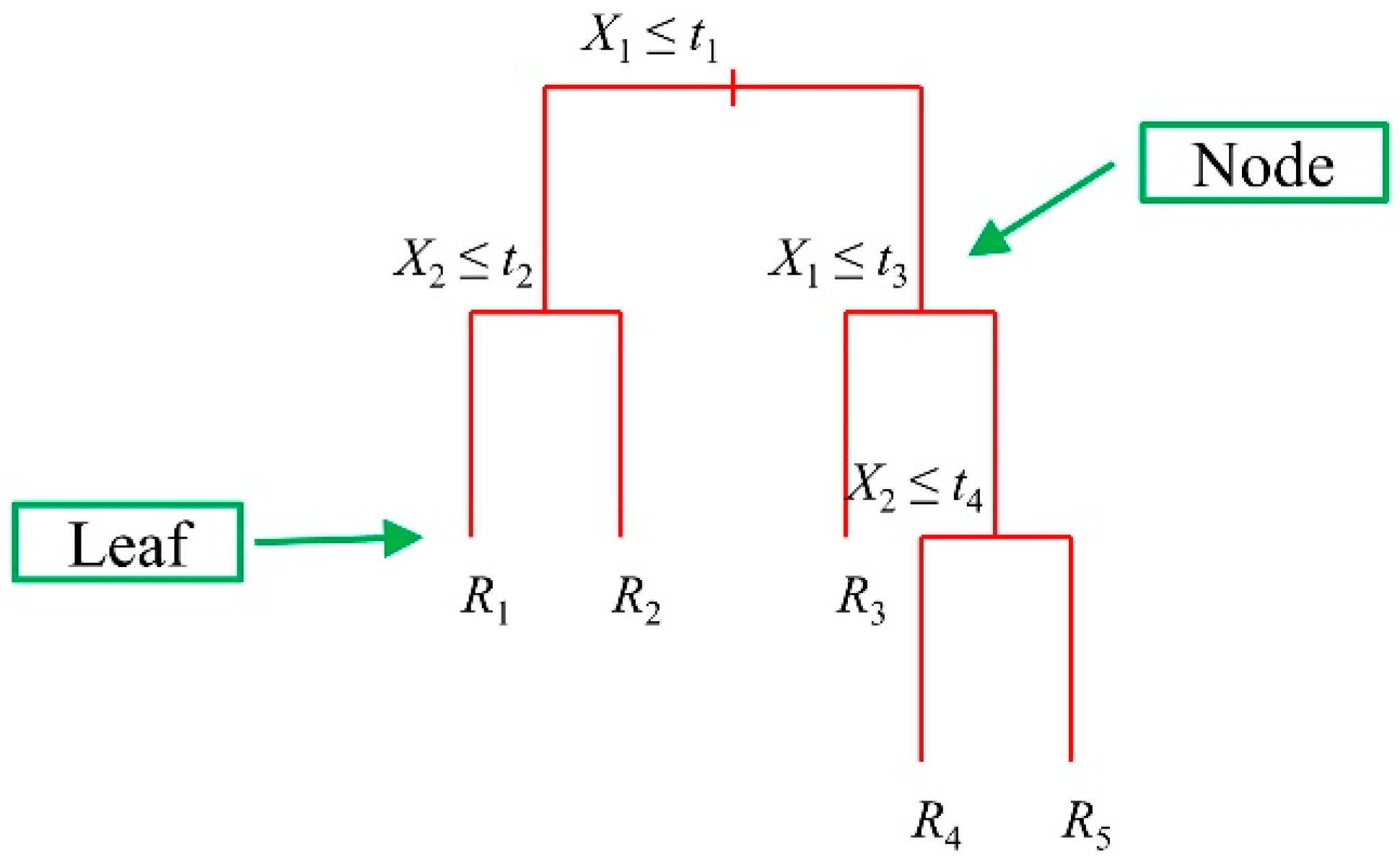
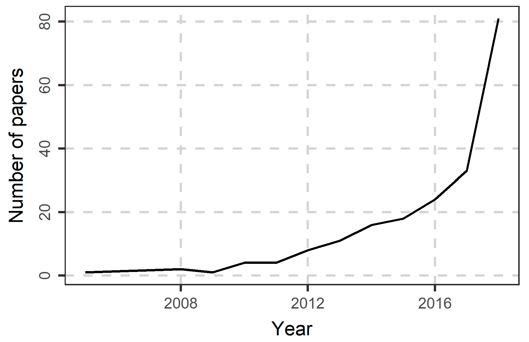
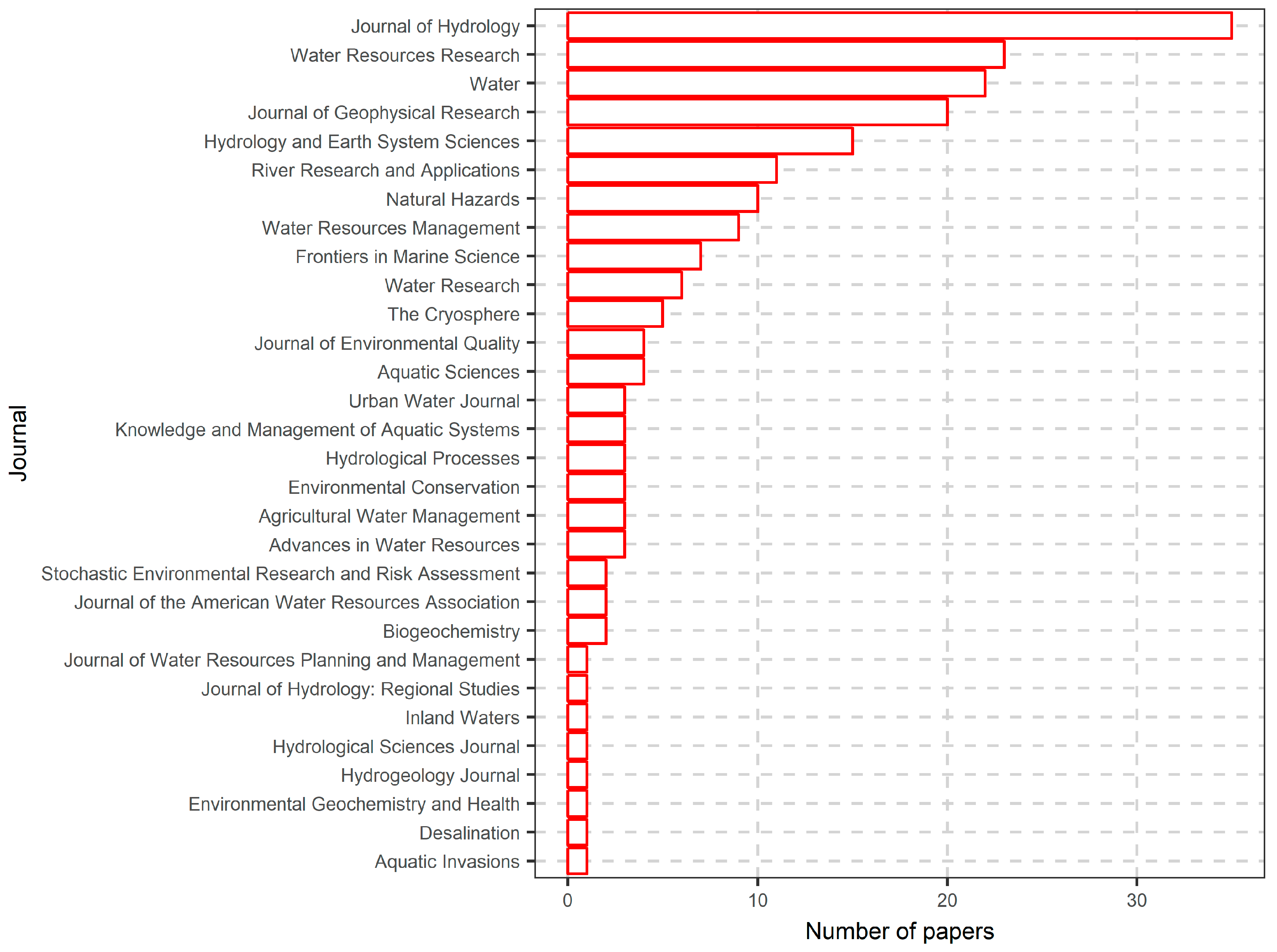
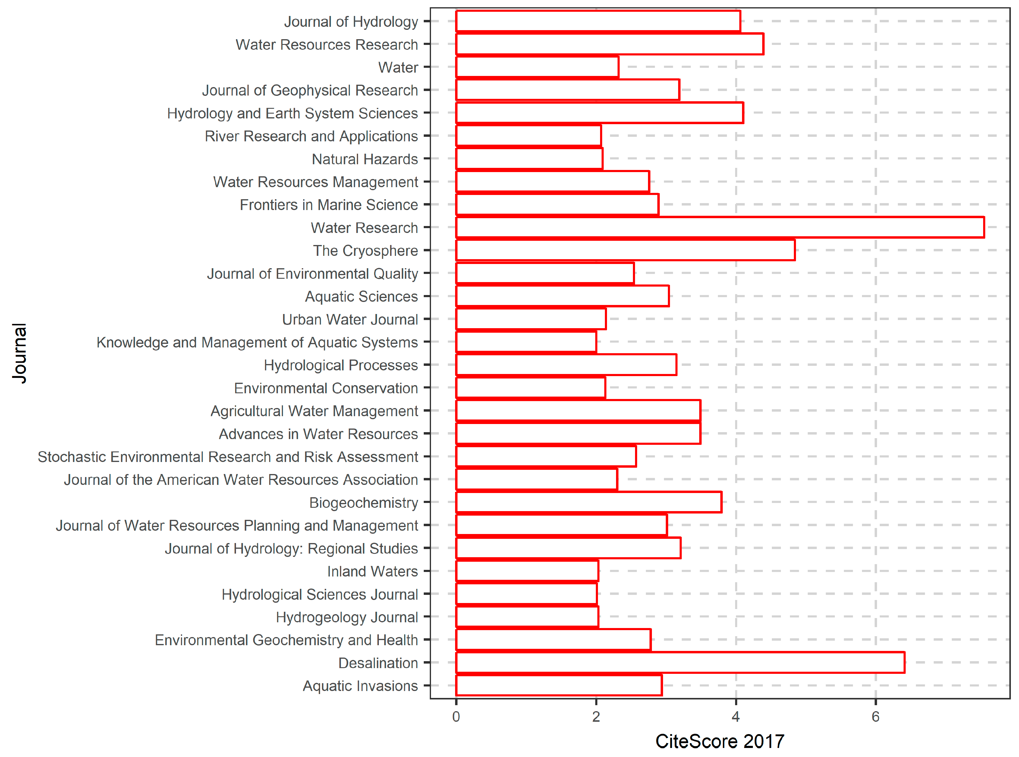
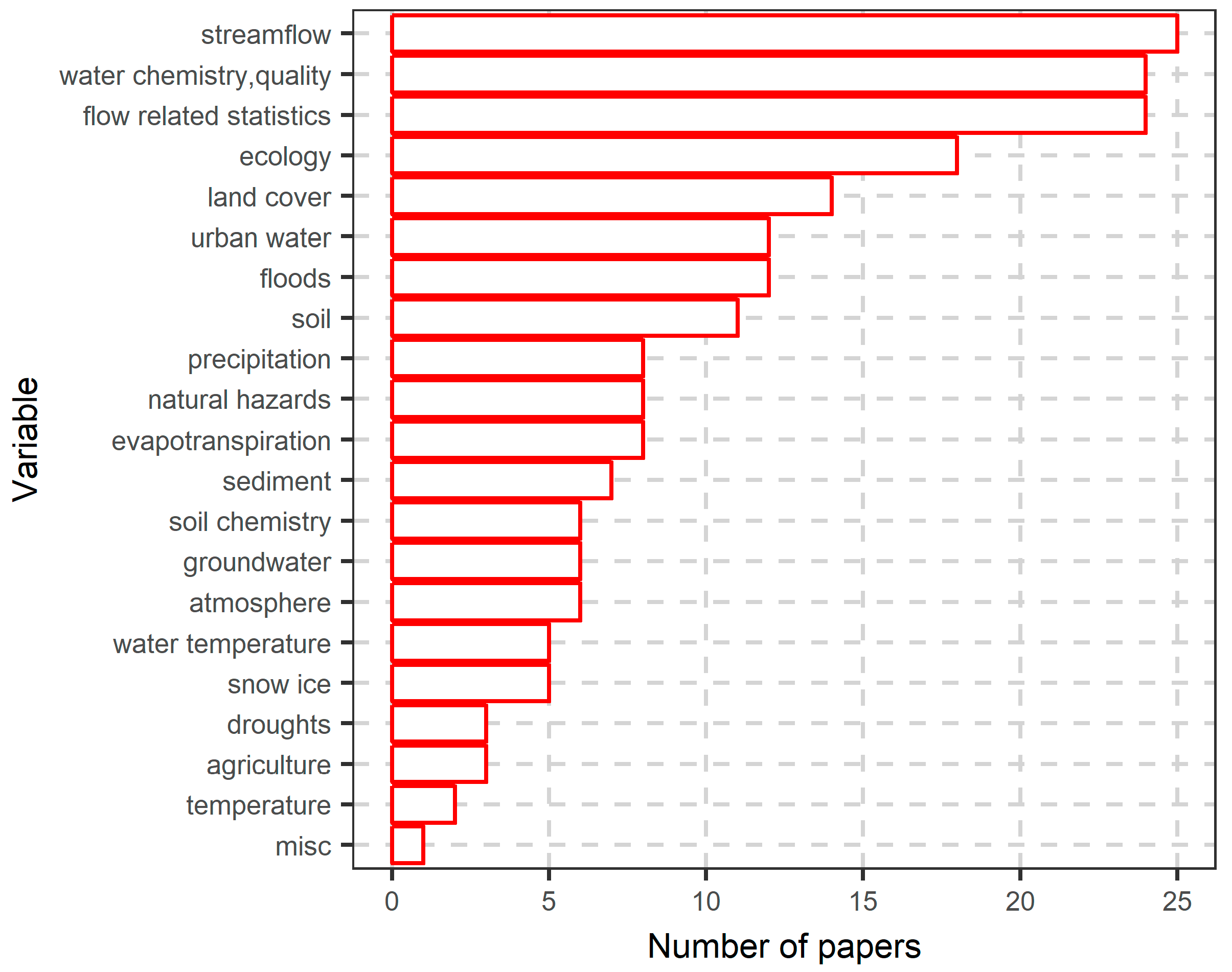
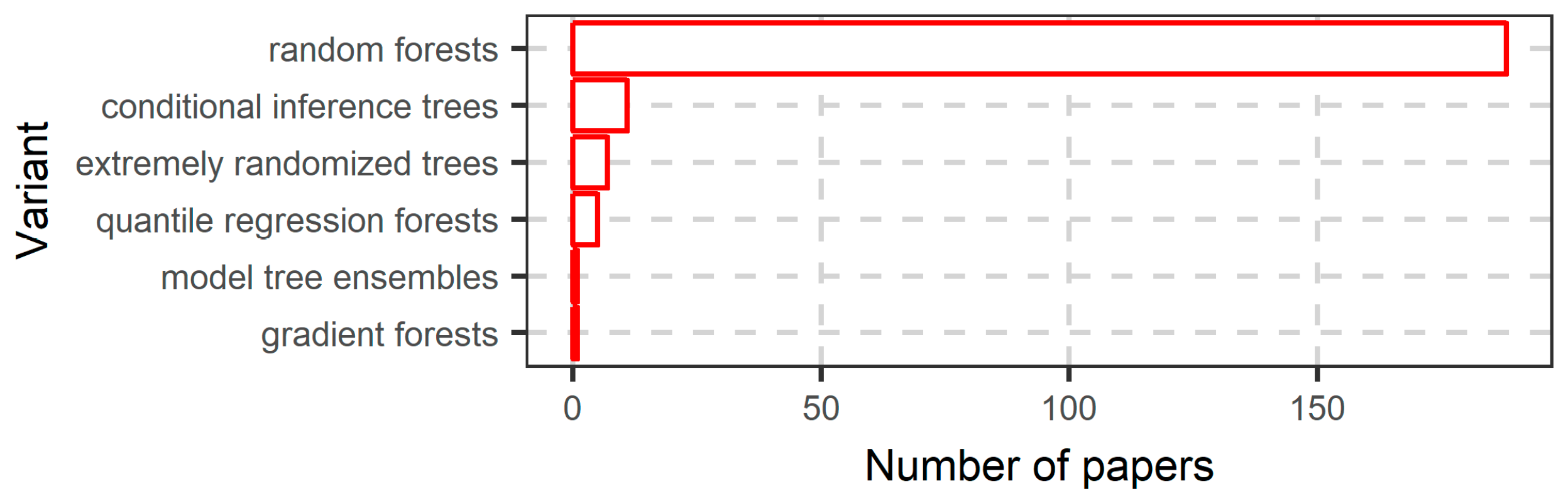
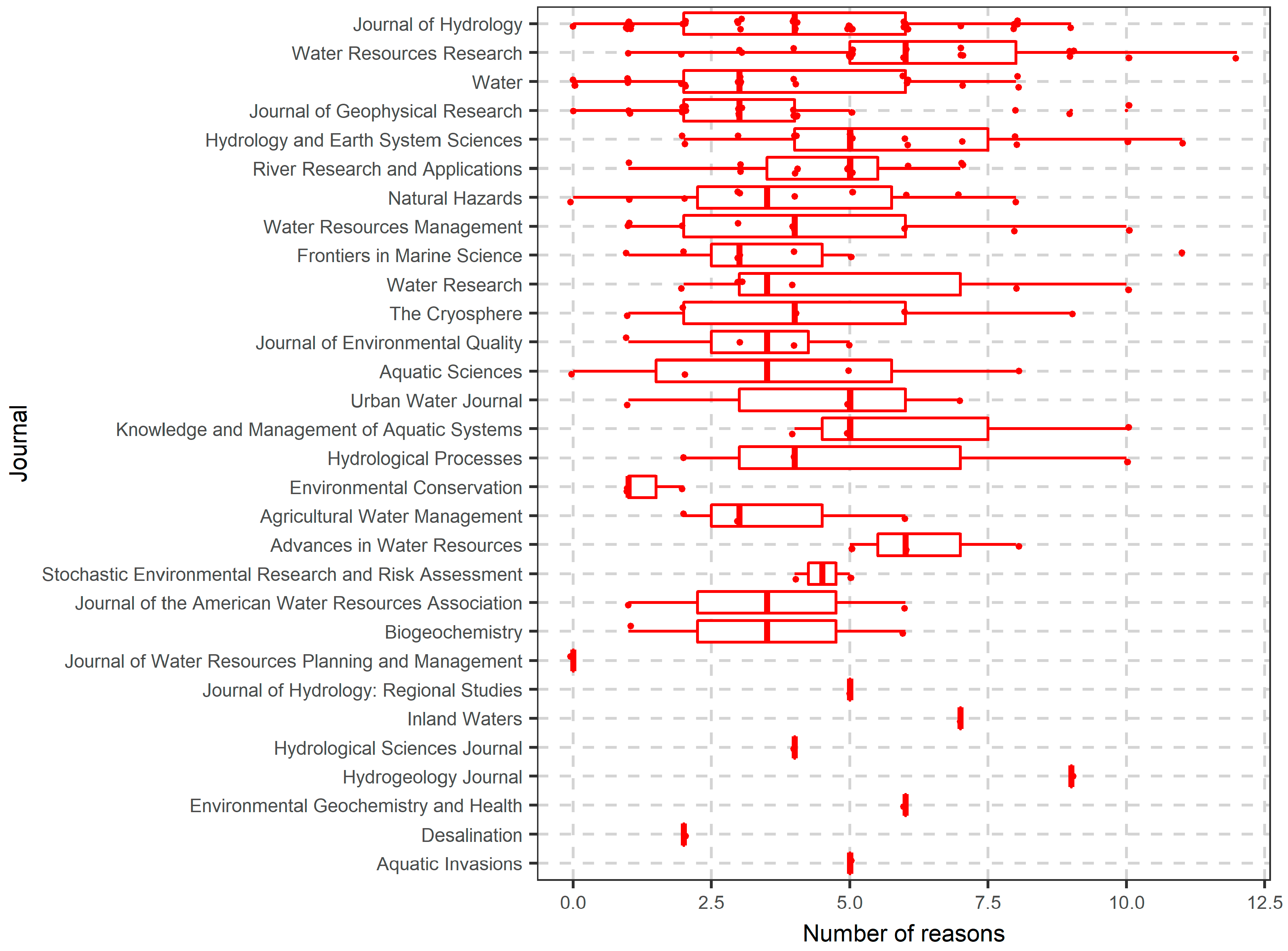
Table 1.
Reviews of data-driven models in water resources.
| Paper | Algorithms | General Theme | Topics Examined |
|---|---|---|---|
| [21] | Artificial neural networks | Rainfall-runoff modeling and flood forecasting | Preprocessing, variable selection, training, testing, modeling practices |
| [22,23] | Artificial neural networks | Water resources applications | Methods for variable selection |
| [20] | Artificial neural networks, genetic programming, evolutionary regression, fuzzy-rule based systems, support vector machines, chaos theory, instance-based learning, regression trees | River flow forecasting, river basin flow prediction, contaminant transport | Testing, human expertise, uncertainty estimation, hybrid models |
| [24] | Artificial neural networks | Rainfall-runoff modeling | Variable selection, training, testing, hybrid models, extrapolation |
| [25] | Artificial neural networks | Flow, salinity, level, nitrate, SO4, drought index, sediment, volume, turbidity, specific conductance, DO, pH, water temperature, concentration of tracer, runoff, river discharge, Secchi depth, Chl a, phosphorus, ammonia, fecal coliform, water supply, debris flow, dam inflow | Variable selection, training, testing, model architecture |
| [26] | Bayesian networks | Environmental modeling | Preprocessing, training, testing, software |
| [27] | Artificial neural networks | Rainfall-runoff, river flow forecasting | Model architecture, preprocessing, variable selection, training, testing, physical interpretation, modular solutions, ensemble learning, hybrid models, benchmark datasets, diagnostics, operational models, uncertainty estimation |
| [28] | Wavelet-Artificial intelligence models | Precipitation modeling, flow forecasting, rainfall-runoff modeling, sediment modeling, groundwater modeling, hydroclimatologic applications | Reviews of data-driven models, testing, usefulness of hybrid wavelet-based models |
| [29] | Support vector machine | Rainfall forecasting, runoff forecasting, streamflow forecasting, sediment yield forecasting, evaporation and evapotranspiration forecasting, lake and water level forecasting, flood forecasting, drought forecasting, groundwater level forecasting, soil moisture estimation, groundwater quality assessment | Mostly comparison of studies |
| [30] | Ant colony optimization | Optimization, reservoir operation and surface water management, water distribution systems, drainage and wastewater engineering, groundwater systems including remediation, monitoring, and management, Environmental and Watershed Management Problems, other applications | Analysis of the literature |
| [31] | Artificial neural networks, fuzzy logic networks, genetic algorithms, genetic programming, particle swarm optimization, honey-bee mating, artificial bee colony | Inflow forecasting, reservoir management optimization | General evaluation of the algorithms |
| [32] | Artificial neural networks, support vector machine, fuzzy logic, evolutionary computing, wavelet-artificial intelligence model | Streamflow forecasting | General evaluation of the algorithms |
| [33] | Artificial neural networks, adaptive neuro fuzzy inference system, other algorithms, wavelet-artificial intelligence model | Sediment transport | General evaluation of the algorithms |
| [34] | Bayesian belief networks | Environmental applications | Geographic distribution of papers, data sources, testing, climate change related issues, water resources management, integration with other models |
| [35] | Artificial neural networks | Forecasting of water related variables, uncertainty estimation | General evaluation of methods for uncertainty estimation, testing |
| [36] | Genetic programming | Rainfall-runoff modeling, streamflow forecasting, water quality variables modeling, groundwater modeling, soil properties modeling, sediment transport, reservoir flow prediction, pipeline flow prediction, open channel flow, wave height prediction, statistical downscaling, precipitation, evaporation, evapotranspiration, solar radiation, drought forecasting, temperature | Evaluation of the applications, selection of parameters |
| [37] | Deep learning | Water resources related problems | General discussion |
| [38] | ARIMA, ARMAX, linear regression, support vector machine, genetic programming, fuzzy logic, hybrid models | Univariate streamflow forecasting | General evaluation of the algorithms |
Table 2.
Variants of random forests.
| Variant | Reference | Characteristic |
|---|---|---|
| Quantile regression forests | [85] | Quantile regression |
| Extremely randomized trees | [103] | They split nodes by choosing cut-points fully at random and use the full learning sample to grow the trees. It corresponds to a lower parametric version of random forests |
| Enriched random forests | [104] | Weighted random selection of predictor variables as candidates for splitting. |
| Rotation forests | [105] | Combines splitting of the predictor variables set with principal component analysis for improved accuracy |
| Conditional inference forests | [71,100,106,107,108] | Unbiased variable importance measures in the case of correlated or mixed type (i.e., continuous and categorical) predictor variables. |
| Random survival forests | [98,109,110] | Survival analysis. |
| Online forests, Mondrian forests. information forests | [111,112,113,114] | Handles training data arriving sequentially or continuously, changing the underlying distribution. |
| Ranking forests | [115,116] | Ranking problems |
| Random ferns | [117] | Same test parameters are used in all nodes of the same tree level. It corresponds to a lower parametric version of random forests. |
| Bayesian additive regression trees | [94] | Aggregation of trees, but inference and fitting is accomplished using Bayesian methods. Conditional means and quantiles can be computed. |
| Node harvest | [118] | Multiple single nodes. |
| Density forests | [15] | Density estimation of unlabeled data. |
| Manifold forests | [15] | Manifold learning (dimensionality reduction). |
| Semi-supervised forests | [15] | Semi-supervised learning. |
| Entangled forests | [119] | Entanglement of the tests applied at each tree node with other nodes in the forest. |
| Decision tree fields | [99] | Combination of random forests and random fields. |
| STAR model | [120] | They can be seen as single nodes equipped with one random projection and multiple decision thresholds |
| Multivariate random forests | [97] | Predicts multiple dependent variables. |
| Dynamic random forests | [121] | Inclusion of trees in the ensemble learner depending on previous outputs. |
| Gradient forests | [122] | Use of alternative importance measures. |
| Regularized random forests | [123,124] | Improvements on variable selection within trees. |
| Cluster forests | [125] | Appropriate for clustering (unsupervised learning). |
| Weighted random forests | [126] | Incorporates tree-level weights for more accurate prediction and computation of variable importance. |
| Random intersection trees | [101] | High-order interaction discovery. |
| Hyper-Ensemble Smote Undersampled Random Forests | [91] | Undersampling of the majority class and oversampling of the minority class to learn from highly imbalanced data. |
| Integrated multivariate random forests | [127] | Integrated different data subtypes. |
| Generalized random forests | [89] | Generalization of random forests for adaptive, local estimation. |
| Iterative random forests | [102,128] | High-order interaction discovery. |
| Heteroscedastic Bayesian additive regression trees | [95] | Bayesian additive regression trees for modeling heteroscedastic data. |
| Local linear forests | [129] | They model smooth signals and fix boundary bias issues. They build on generalized random forests. |
| Distributional regression forests | [96] | Version of generalized additive models for location, scale, and shape parameters (GAMLSS), using trees. |
| Causal forests | [92] | Estimation of heterogeneous treatment effects. They can be used for statistical inference. |
| Neural random forests | [130] | Reformulation of random forests in a neural network setting. |
Table 3.
R packages related to random forests (in alphabetical order), and their specific tasks. The packages can be found in the Comprehensive R Archive Network.
Table 3.
R packages related to random forests (in alphabetical order), and their specific tasks. The packages can be found in the Comprehensive R Archive Network.
| R Package | Characteristics |
|---|---|
| abcrf | Combined with other methods |
| AUCRF | Variable selection |
| bartMachine | Variant |
| Boruta | Variable selection |
| CALIBERrfimpute | Imputation |
| caret | Of general use |
| edarf | Utilities |
| extendedForest | Utilities |
| forestControl | Variable selection |
| forestFloor | Utilities |
| funbarRF | Application |
| ggRandomForests | Utilities |
| gradientForest | Variant |
| grf | Variant |
| hyperSMURF | Variant |
| IntegratedMRF | Variant |
| IPMRF | Variable importance |
| iRafNet | Variant |
| iRF | Variant |
| JRF | Variant |
| m2b | Application |
| MAVTgsa | Application |
| metaforest | Application |
| missForest | Imputation |
| mlr | Of general use |
| mobForest | Application |
| ModelMap | Utilities |
| MultivariateRandomForest | Variant |
| obliqueRF | Variant |
| OOBCurve | Utilities |
| ParallelForest | Better programmed |
| party | Variant |
| partykit | Variant |
| pRF | Variable importance |
| quantregForest | Variant |
| randomForest | Variant |
| randomForestExplainer | Variable importance |
| randomForestSRC | Variant |
| ranger | Better programmed |
| Rborist | Better programmed |
| RFgroove | Variable importance |
| RFmarkerDetector | Application |
| rfPermute | Variable importance |
| rfUtilities | Utilities |
| roughrf | Imputation |
| RRF | Variant |
| snpRF | Variant |
| Sstack | Application |
| SuperLearner | Of general use |
| trimTrees | Variant |
| tuneRanger | Utilities |
| varSelRF | Variable selection |
| vita | Variable importance |
| VSURF | Variable selection |
| wsrf | Variant |
© 2019 by the authors. Licensee MDPI, Basel, Switzerland. This article is an open access article distributed under the terms and conditions of the Creative Commons Attribution (CC BY) license (http://creativecommons.org/licenses/by/4.0/).
Share and Cite
MDPI and ACS Style
Tyralis, H.; Papacharalampous, G.; Langousis, A. A Brief Review of Random Forests for Water Scientists and Practitioners and Their Recent History in Water Resources. Water 2019, 11, 910. https://0-doi-org.brum.beds.ac.uk/10.3390/w11050910
AMA Style
Tyralis H, Papacharalampous G, Langousis A. A Brief Review of Random Forests for Water Scientists and Practitioners and Their Recent History in Water Resources. Water. 2019; 11(5):910. https://0-doi-org.brum.beds.ac.uk/10.3390/w11050910
Chicago/Turabian StyleTyralis, Hristos, Georgia Papacharalampous, and Andreas Langousis. 2019. "A Brief Review of Random Forests for Water Scientists and Practitioners and Their Recent History in Water Resources" Water 11, no. 5: 910. https://0-doi-org.brum.beds.ac.uk/10.3390/w11050910
Note that from the first issue of 2016, this journal uses article numbers instead of page numbers. See further details here.