Equivalent Discharge Coefficient of Side Weirs in Circular Channel—A Lazy Machine Learning Approach


Department of Civil and Mechanical Engineering, University of Cassino and Southern Lazio, via G. Di Biasio 43, 03043 Cassino (FR), Italy
*
Author to whom correspondence should be addressed.
Water 2019, 11(11), 2406; https://0-doi-org.brum.beds.ac.uk/10.3390/w11112406
Submission received: 22 August 2019
/
Revised: 9 November 2019
/
Accepted: 14 November 2019
/
Published: 16 November 2019
(This article belongs to the Section Hydraulics and Hydrodynamics)
Abstract
:Side weirs have been widely used since ancient times in many hydraulic works. Their operation can be analyzed following different approaches. However, almost all possible analysis approaches require knowledge of the discharge coefficient, which depends on several geometric and hydraulic parameters. An effective methodology for predicting discharge coefficient can be based on machine learning algorithms. In this research, experimental data obtained from tests carried out on a side weir in a circular channel and supercritical flow have been used to build predictive models of the equivalent discharge coefficient, by which the lateral outflow can be estimated by referring only to the flow depth upstream of the side weir. Four models, different in the input variables, have been developed. Each model has been proposed in 5 variants, depending on the applied algorithm. The focus is mainly on two lazy machine learning algorithms: k Nearest Neighbor and K-Star. The 5-input variables Model 1 and the 4-input variables Model 2 noticeably outperform the 3-input variables Model 3 and Model 4, showing that a suitable characterization of the side weir geometry is essential for a good accuracy of the prediction model. In addition, under models 1 and 2, k Nearest Neighbor and K-Star, despite the simpler structure, provide comparable or better performance than more complex algorithms such as Random Forest and Support Vector Regression.
1. Introduction
Side weirs are probably one of the most used hydraulic devices to separate flows in open channels. They have been widely used since ancient times in irrigation, drainage, flood regulation, water treatment and in several other areas of hydraulic and environmental engineering. Although they have been studied for almost a hundred years [1,2,3,4,5,6,7,8], side weirs represent a still open and worthy of investigation topic, especially in the case of supercritical flow.
The analysis of the hydraulic operation of a side weir can be carried out following different approaches: the energy balance approach [1,9], the momentum approach [10,11], the flow power variation approach [12], empirical equations [13], computational fluid dynamics [14,15].
The flow equation needs to be completed by the lateral outflow law [16], therefore almost all possible analysis approaches require knowledge of the discharge coefficient CD, both for the estimation of the lateral outflow, and for the prediction of the free surface along the weir. The problem is far more complex in the case of low-crested side weir [17]. In this latter case, traditional approaches to the analysis of side weirs may lead to unsatisfactory results.
The discharge coefficient depends on several variables: The height and length of the weir, the crest profile (sharp or rounded) the shape of the channel cross section, the flow depth above the weir, the kinematic features of the incoming flow. The discharge coefficient has been the subject of several studies [18,19,20,21,22,23]. In practice it is often assumed that CD is constant along the side weir, however it has been shown experimentally that it actually changes along the weir [24].
An effective approach for predicting discharge coefficient from experimental data may be based on machine learning algorithms. Artificial Intelligence algorithms have been increasingly used in recent years to address hydrology and hydraulics problems [25,26,27,28,29,30,31,32]. Machine learning algorithms have already been used in research concerning side weirs, also with particular reference to discharge coefficient. Emiroglu and Kisi applied adaptive neuro-fuzzy inference system (ANFIS) to predict flow over trapezoidal labyrinth side weirs located on a straight channel [33]. Parsaie and Haghiabi used a multilayer perceptron (MLP) to increase the accuracy of estimation of discharge coefficient of a side weir [34]. Azamathulla et al. employed support vector machine (SVM) to predict the side weir discharge coefficient [35]. Roushangar et al. investigated the potential of two different machine learning approaches, specifically support vector machines combined with genetic algorithm (SVM–GA) and gene expression programming (GEP) for predicting trapezoidal and rectangular sharp-crested side weirs discharge coefficient [36]. Azimi et al. performed a sensitivity analysis of the factors that affect the discharge capacity of side weirs in trapezoidal channels by means of extreme learning machines [37].
In this work, experimental data obtained from tests conducted on a side weir in a circular channel and supercritical flow have been used to develop predictive models of the discharge coefficient. In particular, an “equivalent” discharge coefficient CDe has been considered. The adjective “equivalent” refers to the fact that discharge coefficient is evaluated by considering only the flow depth upstream of the side weir, not to the actual flow depths along the side weir. In this way, the side weir can be assimilated to a simple weir. Four models, different in the input variables, were built. Each model was developed in 5 variants, depending on the implemented algorithm. The focus was mainly on two lazy machine learning algorithms: k Nearest Neighbor and K-Star. The main advantage of a lazy machine learning method is that the target function is approximated locally, therefore a lazy learning system can simultaneously solve multiple problems and deal effectively with changes in the problem domain.
Their application to problems of this type is one of the main innovative elements of this work. They were then compared with more complex and more widely used algorithms, such as Random Forest, Support Vector Regression, and Multilayer Perceptron, showing satisfactory performances.
2. Materials and Methods
In the following the experimental setup and the algorithms implemented in the models are described. The main purpose of this work is to show the effectiveness of two lazy machine learning algorithms in predicting the discharge coefficient of a side weir in supercritical flow and circular channel. These algorithms have been chosen because they are very effective in the case of non-linear problems dependent on few variables and also because they have never been applied to problems concerning wastewater hydraulics. The description of the algorithms is deliberately concise to reserve more space for the results of their application.
2.1. Experimental Setup
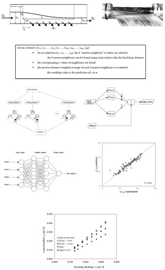
Experiments have been conducted in Water Engineering Laboratory of University of Cassino and Southern Lazio. The experimental setup consists of a recirculation system which supplies a circular plexiglass pipe of internal diameter D = 290 mm with a side weir of variable height (Figure 1). The recirculation system includes: a first supply tank, with the pumps for supplying the second tank, which in turn supplies the pipe, a collecting tank for lateral outflows, and a collecting tank for the downstream flows. The incoming flow rate is measured by means of an electromagnetic flowmeter. The downstream flow rate and the lateral outflow are gauged by V-notch weirs placed on the collecting tanks. The flow depths are measured by some piezometers placed along the pipe.
Four different lengths of side weir have been considered: L = 0.8, 1.0, 1.2, and 1.4 m. For each value of the weir length, the height of the weir crest, w, has been varied from 5 to 11 cm, with a size increment of 1 cm. The incoming flow rate Qo has been varied from 4 L/s to 63 L/s, with an increase of 2 L/s up to 30 L/s, an increase of 3 L/s up to 39 L/s and with an increase of 6 L/s for larger flows rates. The lower flow rates were tested only on lower weir crest height. The corresponding Froude numbers Fo varied from about 1.05 to about 1.70. Overall, the results of more than 450 selected experimental tests were used in this study.
2.2. k Nearest Neighbor and K-Star
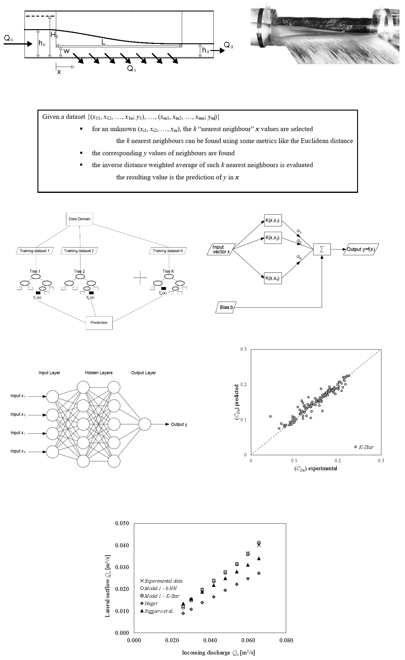
The k Nearest Neighbor (k-NN) is a non-parametric, instance based, lazy supervised algorithm [38]. It is a very simple but fundamental procedure, often used as a benchmark for more complex predictive algorithms. Despite its simplicity, k-NN can outperform more powerful procedures. It was initially used for classification problems: In this case the algorithm provides a class membership as output. An object is classified on the basis of the membership of its neighbors: The object is assigned to the most common class among its k nearest neighbors, where k is a generally small positive integer.
In k-NN regression, the algorithm is used for approximating continuous variables. It can be used a weighted average of the k nearest neighbors’ values, weighted by the inverse of their distance. The Euclidean distance is commonly used as distance metric. Therefore, instead of assigning a label, a real value based on the average of all the neighbors is obtained. Figure 2 shows a pseudocode of the algorithm.
Predictions are made for a new instance by searching through the entire training set for the k most similar instances (the neighbors) and summarizing the output variable for those k instances. For regression this is the mean output variable.
The training set consists of vectors in a multidimensional feature space, each with a target value, while the training process involves only the feature vectors storing and target values of the training samples. The optimal selection of k is depending on data: k = 3 proved to be the optimal value in this study for all considered models. The accuracy of the k-NN algorithm can considerably decrease due to the presence of irrelevant or noisy features, or if the feature scales are not consistent with their prominence.
The K-Star algorithm is an instance-based procedure too and it is very similar to the k-NN algorithm above introduced. The innovative feature introduced by Cleary and Trigg is represented by the use of an entropy metric instead of the classical Euclidean metric [39]. The insight is that the distance between different instances can be defined as the complexity of the transformation of one instance into another. The calculation of the complexity is developed through defining a finite set of transformations which map instances to instances and by introducing the K* distance, which is defined as:
where P* is defined as the probability of all paths from instance a to instance b. If the instances are real numbers, it can be shown that P*(b|a) depends only on the absolute difference between a and b. Moreover, it can be shown that:
where i = |a − b| and s is a parameter of the model, which can take a value between 0 and 1. Therefore, the distance is proportional to the absolute difference between two instances. Moreover, for real numbers the hypothesis is assumed that the real space is underlain by a discrete space with the distance between the discrete instances being very small. The first step is to take the expressions above in the limit as s approaches 0. This leads to:
This can be reformulated as a probability density function where the probability to generate an integer between i and i + i is:
That can be rescaled in terms of a real value x, where , leading to the probability density function over the real numbers:
Practical applications need a reasonable value of xo, which is the mean expected value for x over the distribution P. In the K-Star algorithm, xo is selected by choosing a number between no and N, where N is the total number of training instances and no is the number of the training instances at the smallest distance from a. It is convenient to choose the number by referring to the “blending parameter” b, which varies from b = 0%, for no and b = 100%, for N, with intermediate values interpolated linearly. For more details on the algorithms [39]. In this study a value of b = 20% has been assumed.
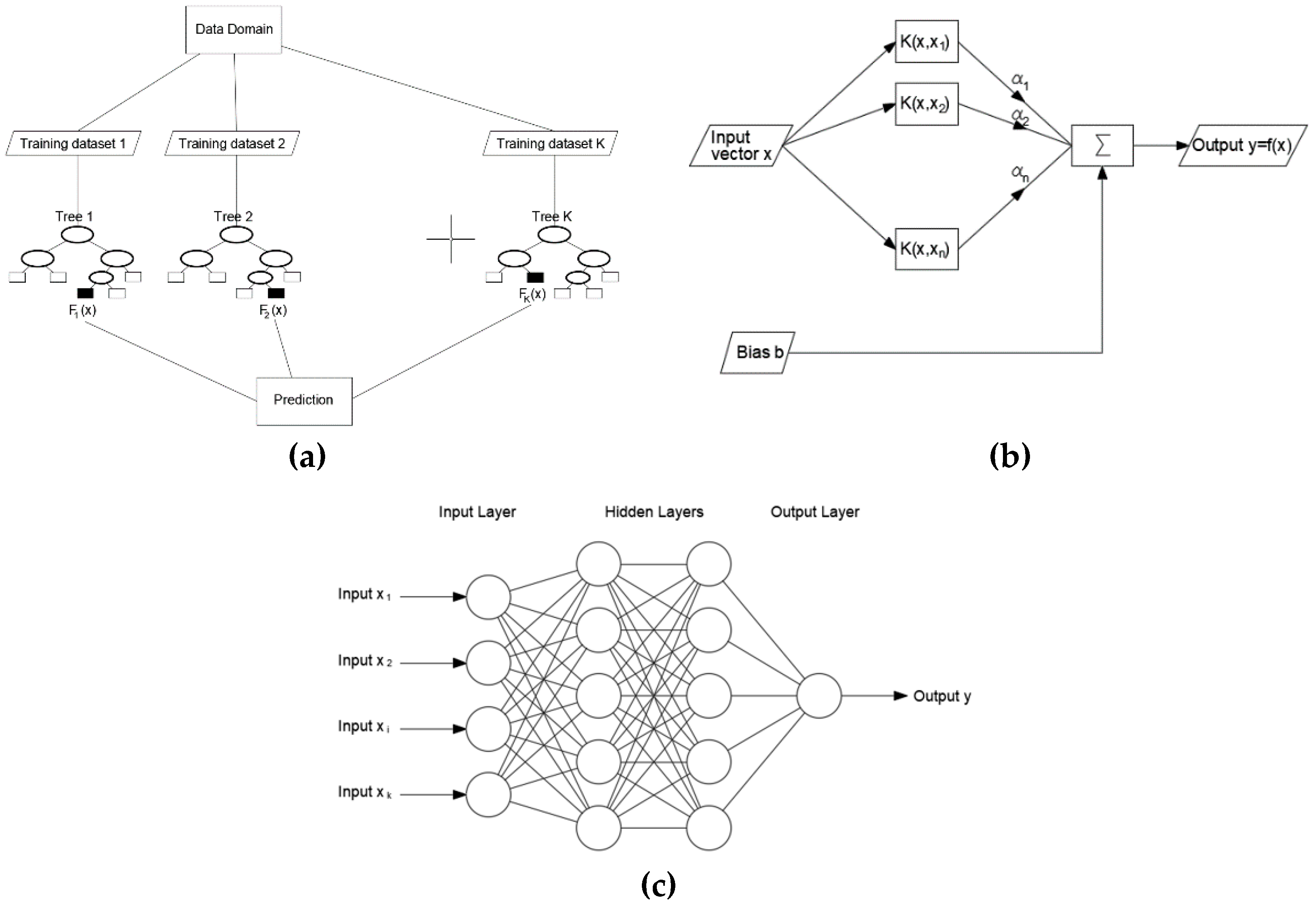
2.3. Random Forest
A Random Forest is a powerful ensemble model. It is achieved by combining a set of uncorrelated, simple Regression Trees [40]. Internal nodes designate the input variables, whereas leaves represent given real values of the target variables. The development of a Regression Tree model consists of the recursive subdivision of the input domain data into subdomains, considering all the possible splits on every field and detecting at each stage the subdivision in two distinct partitions that minimizes the least squared deviation, defined as:
where N(t) is the number of units of sample in the node t, yi is the value assumed by the target variable in the i-th unit and ym is the mean value of the target variable in the node t. R(t) provides an estimation of the “impurity” at each node. A multivariable linear regression model is used to make predictions in each subdomain. The algorithm stops when a stopping rule is met: In this case, lowest impurity provides the stopping rule.
Starting from a training dataset, each tree of the forest is developed from a different bootstrap sample of the data. In addition, in Random Forests the regression trees are developed following a slightly different procedure. Each node can be allocated not referring to the best split among all the input variables but randomly selecting only a part of the variables to split on. The number of these variables is retained constant during the expansion of the forest. Each tree is developed as much as possible. The models considered in this study showed the best accuracies for a number of variables to be considered, for each split, equal to n − 1, if n are the input variables. A slight reduction in the accuracy of the models with decreasing number of variables to split on was observed.
The random forests used in this study consist of 100 trees.
2.4. Support Vector Regression
Given a training dataset {(x1, y1), (x2, y2), …, (xl, yl)} ⊂ X × R, where X is the space of the input patterns (e.g., X = Rn), Support Vector Regression (SVR) is a supervised learning algorithm [41] that aims to find a function f(x) with a maximum ε deviation from the experimental target values yi and as flat as possible. Hence, assumed a linear function in the form:
where w ∈ X, b ∈ R and is the dot product in X, the Euclidean norm ||w||2 has to be minimized, leading to a constrained convex optimization problem. In many cases a certain error has to be tolerated, so it is required to introduce slack variables ξi, ξi∗ in the constraints. Therefore, the optimization problem is formulated as:
where the tolerated deviations and the function flatness depend on the constant C > 0.
SVR can be made nonlinear through a pre-processing of the training patterns xi by means of a function Φ: X→F, where F is some feature space. Since SVR algorithm is only depending on the dot products between the different patterns, it is possible to use a kernel rather than explicitly using the function Φ(·).
In this research, a radial basis function (RBF) was chosen as kernel:
The sequential minimal optimization algorithm is used for solving the quadratic programming problem that arises during the training of support-vector machines. In this research, the following parameter values proved to be a good choice for all the considered models: C = 1, γ = 0.01, ε = 10−4.
2.5. Multilayer Perceptron
A multilayer perceptron (MLP) is a system of simple interconnected nodes, which models a nonlinear relationship between an input vector and an output vector [42]. The nodes, or neurons, are linked by weights and output signals that are a function of the sum of the inputs to the node transformed by a simple nonlinear transfer function. The combination of several simple nonlinear transfer functions allows the MLP to approximate highly non-linear functions. The output of a neuron is scaled by the linking weight and fed forward in order to be an input to the neurons in the next layer of the network. This entails a route of information processing, therefore the MLP is a feed-forward neural network. The architecture of a MLP may significantly vary, but generally it consists of several layers of neurons. The characteristics of the models implemented in this research, in terms of number of hidden layers and number of nodes for each layer, are shown in Table 1.
In this study MLP utilizes a supervised learning technique called backpropagation for training. The activation function is the sigmoid. Number of epochs (iterations) that the back propagation algorithm performs during the training is 500. The adopted learning rate is 0.3. Momentum rate for the backpropagation algorithm is 0.2. The structures summarized in Table 1 proved to be optimal for the investigated problem and for the available dataset. Furthermore, a preliminary sensitivity analysis has shown that the model is not very sensitive to parameter variations.
The typical structures of the Random Forest (RF), Support Vector Regression (SVR), and MLP based models are shown in Figure 3.
3. Results and Discussion
In order to easily estimate the lateral outflow, it may be useful to consider an equivalent discharge coefficient CDe, evaluated with reference to the flow depth ho upstream of the side weir:
in which Qs is the lateral outflow, L is the length of the weir, w is the height of the weir crest, and Kc is a correction coefficient. The main advantage of such an approach is to calculate the lateral outflow without considering the actual free surface on the side weir, which in some device configurations can take on a complex shape. In this regard, Kc allows to take into account the factors that accentuate the typical characteristics of the spatially varied flow.
With applicable simplifications, it is possible to assume that:
in which the Ho/w ratio allows to take into account the local effects in velocity, the L/D ratio and the Lw/D2 parameter are representative factors of the relative flow direction over the side weir [9,17].
Equation (11) can be reformulated as follows:
or more concisely:
having set
Equations (12) and (14) allow to state:
The incoming flow characteristics are represented by the upstream energy head Ho. However, in the design of side weir, one might think that the lateral outflow should be an output of the model, which should take the incoming flow as input. Therefore, since Qs depends on the incoming flow Qo, as well as the geometrical parameters listed above, it can be written:
The choice to work with dimensionless variables gives superior generalization to the results.
Machine learning algorithms are particularly suitable for identifying complex non-linear relationships such as the one represented by Equation (17). One of the substantial steps in machine learning based model development is the selection of a proper set of input variables from the available candidates [43,44,45]. This is because the performance of data driven models is highly sensitive to the selected input variables. If relevant inputs are omitted, the model can be unable to identify the desired input–output relationships. On the other hand, if the model includes unessential inputs, it might be affected by some drawbacks: e.g., the size, computational complexity and memory requirements of the model increase, model calibration becomes more difficult owing to an increase in the size of the search space, the understanding of physical meaning from calibrated models is more difficult. In this study, the input variables selection has been conducted mainly on a physical basis: Equation (11), which defines the discharge coefficient, and the subsequent developments leading to Equation (17) clearly indicate the input variables to be considered.
Based on the number of input variables, four different models have been developed for the prediction of CDe. Five variants of each model have been built, varying the applied machine learning algorithm. The described algorithms were implemented in MATLAB environment. The search for the optimal structure of the models and their parameters was conducted by means of a trial and error iteration procedure, by varying the values of the parameters of the models and checking the values of the metrics defined below.
Model 1 has the following input variables: Qo*, Γ, Ho/w, L/D, Lw/D2. Model 2 neglects the dimensionless incoming discharge and requires the following input variables: Γ, Ho/w, L/D, Lw/D2. Model 3 and Model 4 both have 3 input variables. Model 3 needs Γ, Ho/w, and Lw/D2, while Model 4 requires Γ, Ho/w, and L/D.
The effectiveness of predictive models has been evaluated by four of the most common metrics: the Nash–Sutcliffe Efficiency (NSE), the Mean Absolute Error (MAE), the Root Mean Squared Error (RMSE), the Relative Absolute Error (RAE). Their definitions are given in Table 2.
Each model was built by means of a k-fold cross validation procedure, with a set of 450 vectors. In k-fold cross validation, the original dataset is randomly partitioned into k subsets. Then, a single subset is reserved as the validation data for testing the model, while the remaining k − 1 subsets are employed as training data. The cross-validation procedure is repeated k times: Each of the k subsets is used once as the validation dataset. Finally, the k results from the folds are averaged to provide a single estimation. In this study, k was chosen equal to 10. This value ensures satisfactory results.
The results achieved, with particular reference to the effectiveness of the models, are summarized in Table 3.
CDe values are lower than those commonly assumed by the discharge coefficient, because they are evaluated with reference to the upstream flow depth.
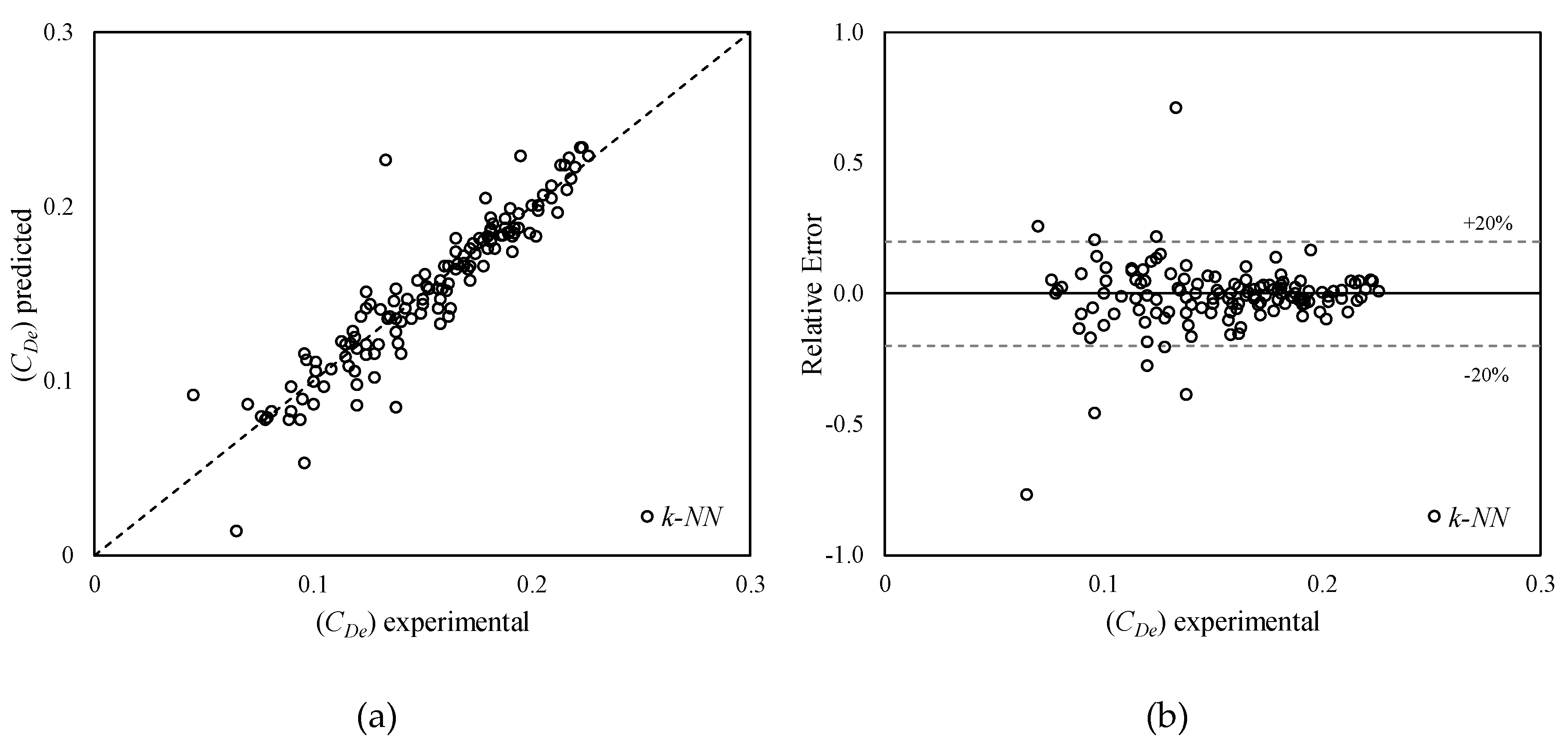
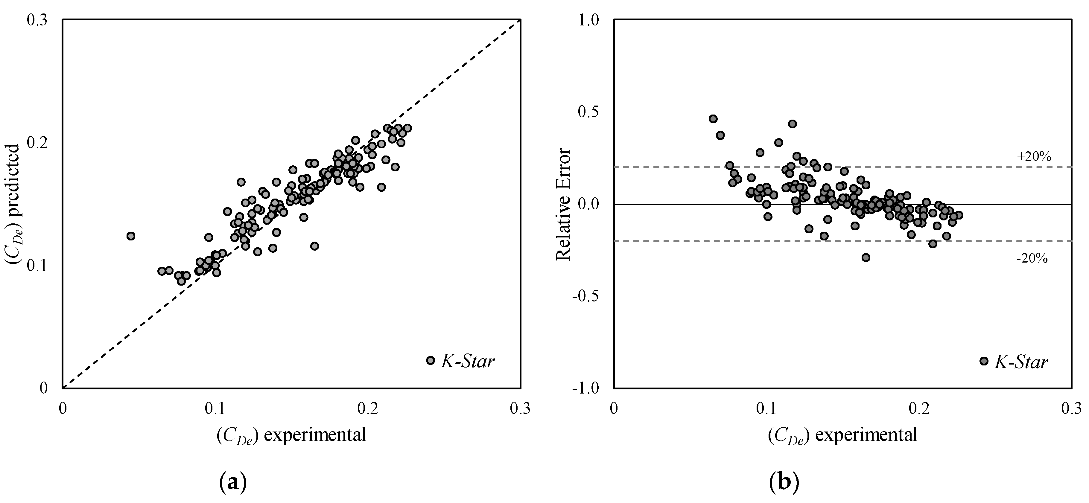
Model 1 provides the best results for almost all the considered algorithms. Lazy machine learning algorithms show very good predictive capabilities and K-Star algorithm (NSE = 0.912, MAE = 0.0075, RMSE = 0.0119, RAE = 21.7%) clearly outperforms k-NN algorithm (NSE = 0.863, MAE = 0.0103, RMSE = 0.0159, RAE = 29.8%). The latter (Figure 4) shows the highest relative errors for CDe less than about 0.15, while the error distribution appears to be quite symmetrical. On the other hand, K-Star (Figure 5) tends to overestimate CDe when it is less than about 0.12. However, even in this case the highest errors occur for CDe less than about 0.15.
RF (NSE = 0.865, MAE = 0.0089, RMSE = 0.0147, RAE = 26.0%) slightly outperforms k-NN, while SVR (NSE = 0.784, MAE = 0.0128, RMSE = 0.0186, RAE = 37.2%) underperform the models shown above. Both RF and SVR (Figure 6 and Figure 7) show the highest relative errors for CDe less than about 0.13. In particular, SVR shows a tendency to overestimate the actual values in that range.
MLP leads to the least accurate predictions among all developed models (NSE = 0.602, MAE = 0.0232, RMSE = 0.0314, RAE = 67.5%). The errors are considerably higher and a general tendency to overestimate the experimental data is observed (Figure 8).
Model 2 provides slightly worse results, but still comparable to those of Model 1. The absence among the input variables of the dimensionless incoming flow Qo* does not considerably affect the models and their results. In this case k-NN (NSE = 0.857, MAE = 0.0105, RMSE = 0.0161, RAE = 30.6%) leads to the best outcomes. Also in this case k-NN (Figure 9) provides the highest relative errors for CDe less than about 0.15, while the error distribution is quite symmetrical. K-Star (NSE = 0.845, MAE = 0.0117, RMSE = 0.0166, RAE = 34.1%), on the other hand, shows performances in line with those of RF (NSE = 0.843, MAE = 0.0110, RMSE = 0.0159, RAE = 32.1%). Both algorithms (Figure 10 and Figure 11) tend to overestimate CDe, with the highest errors if it is less than about 0.15. If CDe is greater than 0.15, the predictions are very accurate. The RF-based Model 2 outperforms the RF-based Model 1. The usage of SVR (Figure 12) in Model 2 leads to similar trends to those found for K-Star and RF, but forecast accuracy is lower (NSE = 0.721, MAE = 0.0150, RMSE = 0.0213, RAE = 43.5%). Finally, MLP leads again to the poorest predictions among all built models (NSE = 0.587, MAE = 0.0218, RMSE = 0.0304, RAE = 63.4%), with considerably higher errors and a clear tendency to overestimate the actual data (Figure 13).
A further effective comparison among the different models is obtained using Taylor diagrams (Figure 14). A Taylor diagram provides a summary statistical representation of the model results in terms of standard deviation, root mean square difference and correlation coefficient with experimental data [46]. The representative points of the most accurate models are closer to the point of the observed data. For Model 1, the better predictive capability of the K-Star algorithms is again evident, while for Model 2 the comparable accuracies of k-NN, K-Star, and RF are noted.
Model 3, which does not include the parameter L/D among the input variables, and Model 4, which does not include the parameter Lw/D2, are characterized by a severe reduction in prediction accuracy. These models are not useful for practical applications. Regarding the Model 3, the variant based on the k-NN algorithm outperforms all the other variants, while K-Star is outperformed by both RF and SVR. On the other hand, MLP provides poor results. As for the Model 4, k-NN and K-Star provide comparable results, but they are both outperformed by RF and SVR. Finally, once again MLP proves to be the least effective algorithm for this problem.
Having shown that the parameters L/D and Lw/D2 are both essential among the input variables to obtain satisfactory results, for the sake of brevity no graphs relating to Model 3 and Model 4 are shown.
The models 1 and 2 based on the considered lazy machine learning algorithms have been finally compared with other models acknowledged in the technical literature: the model proposed by Hager [9], and the empirical equation of Biggiero [13]. The formulation proposed by Hager is a physically based approach, which considers an energy balance along the side weir and leads to the following differential equations:
in which m = 1.4 and
Instead, the empirical equation proposed by Biggiero is the following:
The comparison has been made with reference to the actual lateral outflow. These models were considered suitable for the comparison because both relate to circular pipes and supercritical flows. Figure 15 shows the results of the comparison for some selected experiments. Lazy machine learning algorithms led to results in very good agreement with the experimental results in the entire considered ranges of flow rates. The Hager model tends to underestimate the lateral outflow in the entire investigated experimental range, while the empirical equation of Biggiero tends to underestimate higher lateral outflow values. In particular, the tendency of the Biggiero equation to underestimate higher lateral outflows becomes more evident as the L/w ratio increases (Figure 15).
The proposed approach allows to calculate the lateral outflow from a low crested side weir based on the geometric characteristics of the weir and the hydrodynamic characteristics of incoming flow, without having to previously get the profile of the free surface on the weir. Such an approach can be very useful in both verification and design problems. Machine learning algorithms have proven to be particularly efficient in the development of predictive models of an equivalent discharge coefficient. Furthermore, lazy machine learning algorithms, with a simpler structure, provide comparable performance or in some cases outperform more complex algorithms such as Random Forest and Support Vector Regression. Lazy machine learning algorithms are a good solution to non-linear regression problems with few input variables.
Traditional approaches to the study of side weirs have significant limitations in the case of low crested weirs. The momentum balance methodology is usually accurate enough [11] but it needs the experimental assessment of correction coefficients leading to formulations which are difficult to apply in practical use. The energy balance approach, on the other hand, is not as accurate when the upstream free surface is significantly above the weir crest [9,12]. Empirical models, as well known, are effective under conditions similar to those of experimental tests, but may prove ineffective under significantly different conditions. Moreover, all the aforementioned approaches lead to an underestimation of the lateral outflow at the highest inlet flow rates, which are the most interesting from a practical point of view. The machine-learning based models do not suffer from the above limitations and have shown high accuracy in all the investigated operating conditions.
As specified above, the proposed approach has been tested in supercritical flows and circular channels. These conditions represent the current limitation of the research, but they also provide the hints for the straightest future developments, which could consider different hydrodynamic conditions and different channel shapes.
4. Conclusions
The knowledge of an equivalent discharge coefficient allows to evaluate the lateral outflow from a side weir without the need to know the free surface on the weir. Machine learning algorithms may be very effective to build predictive models of an equivalent discharge coefficient. The results of experimental tests carried out on a side weir in a circular channel and supercritical flow at Water Engineering Laboratory of the University of Cassino and Southern Lazio were used to develop four predictive models, different in input variables. Each model was developed in 5 variants, based on the different implemented algorithm. The 5-input variables Model 1 and the 4-input variables Model 2 clearly outperform the 3-input variables Model 3 and Model 4. An adequate characterization of the side weir geometry is essential for a good result of the prediction model of the discharge coefficient. This characterization can be provided by dimensionless parameters resulting from appropriate combinations of the length of the weir, the height of the weir crest, and the pipe diameter.
In addition, under models 1 and 2, k Nearest Neighbor and K-Star, despite the simpler structure, provide comparable performance or outperform more complex algorithms such as Random Forest and Support Vector Regression. On the other hand, the Multilayer Perceptron algorithm has proved to be unsuitable for providing an accurate prediction of discharge coefficient.
The effectiveness of k-NN and K-Star based models has been further demonstrated by comparisons with extensively used literature formulations. In particular, the two considered lazy machine learning algorithms outperform both the empirical equation of Biggiero et al. and the Hager model in the entire experimental range investigated in this research.
Author Contributions
Conceptualization, F.G.; methodology, F.G.; software, F.G.; validation, F.D.N., R.G. and G.d.M.; formal analysis, F.G.; investigation, F.G. F.D.N. and R.G.; resources, F.G.; data curation, F.G.; writing—original draft preparation, F.G.; writing—review and editing, F.D.N., R.G. and G.d.M.; visualization, F.G. and F.D.N.; supervision, F.G.; project administration, F.G.; funding acquisition, G.d.M.
Funding
This research received no external funding
Conflicts of Interest
The authors declare no conflict of interest.
References
- De Marchi, G. Saggio Di Teoria Del Funzionamento Degli Stramazzi Laterali. L Energ. Elettr. 1934, XI, 849–860. (In Italian) [Google Scholar]
- Gentilini, B. Ricerche Sperimentali Sugli Sfioratori Longitudinali. L Energ. Elettr. 1938, XV, 583–595. (In Italian) [Google Scholar]
- Ackers, P. A Theoretical Consideration of Side Weirs as Stormwater Overflows. Hydraulics Paper no 11. Symposium of Four Papers on Side Spillways. Proc. Inst. Civ. Eng. 1957, 6, 250–269. [Google Scholar] [CrossRef]
- Uyumaz, A.; Muslu, Y. Flow Over Side Weirs in Circular Channels. J. Hydraul. Eng. 1985, 111, 144–160. [Google Scholar] [CrossRef]
- Gisonni, C.; Hager, W.H. Short Sewer Sideweir. J. Irrig. Drain. Eng. 1997, 123, 354–363. [Google Scholar] [CrossRef]
- Oliveto, G.; Biggiero, V.; Fiorentino, M. Hydraulic Features of Supercritical Flow Along Prismatic Side Weirs. J. Hydraul. Res. 2001, 39, 73–82. [Google Scholar] [CrossRef]
- Castro Orgaz, O.; Hager, W.H. Subcritical Side-Weir Flow at High Lateral Discharge. J. Hydraul. Eng. 2012, 138, 777–787. [Google Scholar] [CrossRef]
- Michelazzo, G.; Oumeraci, H.; Paris, E. Laboratory Study on 3D Flow Structures Induced by Zero-Height Side Weir and Implications for 1D Modeling. J. Hydraul. Eng. 2015, 141, 04015023. [Google Scholar] [CrossRef]
- Hager, W.H. Supercritical Flow in Circular-Shaped Side Weir. J. Irrig. Drain. Eng. 1994, 120, 1–12. [Google Scholar] [CrossRef]
- Yen, B.C.; Wenzel, H.G. Dynamic Equations for Steady Spatially Varied Flow. J. Hydraul. Div. ASCE 1970, 96, 801–814. [Google Scholar]
- El Khashab, A.; Smith, K.V.H. Experimental Investigation of Flow Over Side Weirs. J. Hydraul. Div. ASCE 1976, 102, 1255–1268. [Google Scholar]
- Granata, F.; De Marinis, G.; Gargano, R.; Tricarico, C. Novel Approach for Side Weirs in Supercritical Flow. J. Irrig. Drain. Eng. 2013, 139, 672–679. [Google Scholar] [CrossRef]
- Biggiero, V.; Longobardi, D.; Pianese, D. Indagine Sperimentale Su Sfioratori Laterali a Soglia Bassa. G. Del. Genio Civ. 1994, 841, 183–199. (In Italian) [Google Scholar]
- Azimi, H.; Shabanlou, S.; Salimi, M.S. Free Surface and Velocity Field in a Circular Channel Along the Side Weir in Supercritical Flow Conditions. Flow Meas. Instrum. 2014, 38, 108–115. [Google Scholar] [CrossRef]
- Aydin, M.C. Investigation of a Sill Effect on Rectangular Side-Weir Flow by Using CFD. J. Irrig. Drain. Eng. 2015, 142, 04015043. [Google Scholar] [CrossRef]
- Hager, W.H. Lateral Outflow Over Side Weirs. J. Hydraul. Eng. 1987, 113, 491–504. [Google Scholar] [CrossRef]
- Chow, V.T. Open-Channel Hydraulics; McGraw-Hill: New York, NY, USA, 1959. [Google Scholar]
- Swamee, P.K. Discharge Equations for Rectangular Sharp Crested Weirs. J. Hydraul. Eng. 1988, 114, 1082–1087. [Google Scholar] [CrossRef]
- Cheong, H. Discharge Coefficient of Lateral Diversion from Trapezoidal Channel. J. Irrig. Drain. Eng. 1991, 117, 461–475. [Google Scholar] [CrossRef]
- Singh, R.; Manivannan, D.; Satyanarayana, T. Discharge Coefficient of Rectangular Side Weirs. J. Irrig. Drain. Eng. 1994, 120, 814–819. [Google Scholar] [CrossRef]
- Swamee, P.K.; Pathak, S.K.; Ali, M.S. Side-Weir Analysis Using Elementary Discharge Coefficient. J. Irrig. Drain. Eng. 1994, 120, 742–755. [Google Scholar] [CrossRef]
- Borghei, S.M.; Jalili, M.R.; Ghodsian, M. Discharge Coefficient for Sharp-Crested Side Weir in Subcritical Flow. J. Hydraul. Eng. 1999, 125, 1051–1056. [Google Scholar] [CrossRef]
- Kaya, N.; Emiroglu, M.E.; Agaccioglu, H.; Agaçcioglu, H. Discharge Coefficient of a Semi-Elliptical Side Weir in Subcritical Flow. Flow Meas. Instrum. 2011, 22, 25–32. [Google Scholar] [CrossRef]
- Granata, F.; Gargano, R.; Santopietro, S. A Flow Field Characterization in a Circular Channel Along a Side Weir. Flow Meas. Instrum. 2016, 52, 92–100. [Google Scholar] [CrossRef]
- Solomatine, D.P.; Xue, Y. M5 Model Trees and Neural Networks: Application to Flood Forecasting in the Upper Reach of the Huai River in China. J. Hydrol. Eng. 2004, 9, 491–501. [Google Scholar] [CrossRef]
- Najafzadeh, M.; Etemad Shahidi, A.; Lim, S.Y. Scour Prediction in Long Contractions Using ANFIS and SVM. Ocean Eng. 2016, 111, 128–135. [Google Scholar] [CrossRef]
- Granata, F.; Papirio, S.; Esposito, G.; Gargano, R.; De Marinis, G. Machine Learning Algorithms for the Forecasting of Wastewater Quality Indicators. Water 2017, 9, 105. [Google Scholar] [CrossRef]
- Granata, F.; De Marinis, G. Machine Learning Methods for Wastewater Hydraulics. Flow Meas. Instrum. 2017, 57, 1–9. [Google Scholar] [CrossRef]
- Granata, F.; Saroli, M.; De Marinis, G.; Gargano, R. Machine Learning Models for Spring Discharge Forecasting. Geofluids 2018, 2018, 8328167. [Google Scholar] [CrossRef]
- Diez Sierra, J.; Del Jesus, M. Subdaily Rainfall Estimation Through Daily Rainfall Downscaling Using Random Forests in Spain. Water 2019, 11, 125. [Google Scholar] [CrossRef]
- Granata, F. Evapotranspiration Evaluation Models Based on Machine Learning Algorithms—A Comparative Study. Agric. Water Manag. 2019, 217, 303–315. [Google Scholar] [CrossRef]
- Saadi, M.; Oudin, L.; Ribstein, P. Random Forest Ability in Regionalizing Hourly Hydrological Model Parameters. Water 2019, 11, 1540. [Google Scholar] [CrossRef]
- Emiroglu, M.E.; Kişi, O. Prediction of Discharge Coefficient for Trapezoidal Labyrinth Side Weir Using a Neuro-Fuzzy Approach. Water Resour. Manag. 2013, 27, 1473–1488. [Google Scholar] [CrossRef]
- Parsaie, A.; Haghiabi, A. The Effect of Predicting Discharge Coefficient by Neural Network on Increasing the Numerical Modeling Accuracy of Flow Over Side Weir. Water Resour. Manag. 2015, 29, 973–985. [Google Scholar] [CrossRef]
- Azamathulla, H.M.; Haghiabi, A.H.; Parsaie, A. Prediction of Side Weir Discharge Coefficient by Support Vector Machine Technique. Water Supply 2016, 16, 1002–1016. [Google Scholar] [CrossRef]
- Roushangar, K.; Khoshkanar, R.; Shiri, J. Predicting Trapezoidal and Rectangular Side Weirs Discharge Coefficient Using Machine Learning Methods. ISH J. Hydraul. Eng. 2016, 22, 1–8. [Google Scholar] [CrossRef]
- Azimi, H.; Bonakdari, H.; Ebtehaj, I. Sensitivity Analysis of the Factors Affecting the Discharge Capacity of Side Weirs in Trapezoidal Channels Using Extreme Learning Machines. Flow Meas. Instrum. 2017, 54, 216–223. [Google Scholar] [CrossRef]
- Aha, D.W.; Kibler, D.; Albert, M.K. Instance-Based Learning Algorithms. Mach. Learn. 1991, 6, 37–66. [Google Scholar] [CrossRef] [Green Version]
- Cleary, J.G.; Trigg, L.E. K*: An Instance-Based Learner Using an Entropic Distance Measure. In Proceedings of the Machine Learning Proceedings, Tahoe, CA, USA, 9–12 July 1995; Elsevier: Amsterdam, The Netherlands, 1995; pp. 108–114. [Google Scholar]
- Breiman, L. Random Forests. Mach. Learn. 2001, 45, 5–32. [Google Scholar] [CrossRef] [Green Version]
- Vapnik, V.N. The Nature of Statistical Learning Theory; Springer Science and Business Media LLC: Berlin, Germany, 1995. [Google Scholar]
- Baum, E.B. On the Capabilities of Multilayer Perceptrons. J. Complex. 1988, 4, 193–215. [Google Scholar] [CrossRef] [Green Version]
- Bowden, G.J.; Maier, H.R.; Dandy, G.C. Input Determination for Neural Network Models in Water Resources Applications. Part 1. Background and Methodology. J. Hydrol. 2005, 301, 75–92. [Google Scholar] [CrossRef]
- Fernando, T.; Maier, H.; Dandy, G.; Maier, H. Selection of Input Variables for Data Driven Models: An Average Shifted Histogram Partial Mutual Information Estimator Approach. J. Hydrol. 2009, 367, 165–176. [Google Scholar] [CrossRef]
- Galelli, S.; Humphrey, G.B.; Maier, H.R.; Castelletti, A.; Dandy, G.C.; Gibbs, M.S. An Evaluation Framework for Input Variable Selection Algorithms for Environmental Data-Driven models. Environ. Model. Softw. 2014, 62, 33–51. [Google Scholar] [CrossRef] [Green Version]
- Taylor, K.E. Summarizing Multiple Aspects of Model Performance in a Single Diagram. J. Geophys. Res. Space Phys. 2001, 106, 7183–7192. [Google Scholar] [CrossRef]
Figure 1.
Experimental facility. Side weir sketch with symbols. Typical free surface on the side weir in supercritical flow.
Figure 1.
Experimental facility. Side weir sketch with symbols. Typical free surface on the side weir in supercritical flow.

Figure 2.
k Nearest Neighbor (k-NN) algorithm pseudocode. It is also valid for K-Star, as long as the Euclidean metric is replaced by the entropy metric.
Figure 2.
k Nearest Neighbor (k-NN) algorithm pseudocode. It is also valid for K-Star, as long as the Euclidean metric is replaced by the entropy metric.

Figure 3.
Typical architecture of (a) Random Forest, (b) Support Vector Regression, (c) Multilayer Perceptron.
Figure 3.
Typical architecture of (a) Random Forest, (b) Support Vector Regression, (c) Multilayer Perceptron.

Figure 4.
Model 1, k-NN algorithm, (a) predicted versus experimental results, and (b) relative error versus experimental results.
Figure 4.
Model 1, k-NN algorithm, (a) predicted versus experimental results, and (b) relative error versus experimental results.

Figure 5.
Model 1, K-Star algorithm, (a) predicted versus experimental results, and (b) relative error versus experimental results.
Figure 5.
Model 1, K-Star algorithm, (a) predicted versus experimental results, and (b) relative error versus experimental results.

Figure 6.
Model 1, RF algorithm, (a) predicted versus experimental results, and (b) relative error versus experimental results.
Figure 6.
Model 1, RF algorithm, (a) predicted versus experimental results, and (b) relative error versus experimental results.

Figure 7.
Model 1, SVR algorithm, (a) predicted versus experimental results, and (b) relative error versus experimental results.
Figure 7.
Model 1, SVR algorithm, (a) predicted versus experimental results, and (b) relative error versus experimental results.

Figure 8.
Model 1, MLP algorithm, (a) predicted versus experimental results, and (b) relative error versus experimental results.
Figure 8.
Model 1, MLP algorithm, (a) predicted versus experimental results, and (b) relative error versus experimental results.

Figure 9.
Model 2, k-NN algorithm, (a) predicted versus experimental results, and (b) relative error versus experimental results.
Figure 9.
Model 2, k-NN algorithm, (a) predicted versus experimental results, and (b) relative error versus experimental results.

Figure 10.
Model 2, K-Star algorithm, (a) predicted versus experimental results, and (b) relative error versus experimental results.
Figure 10.
Model 2, K-Star algorithm, (a) predicted versus experimental results, and (b) relative error versus experimental results.

Figure 11.
Model 2, RF algorithm, (a) predicted versus experimental results, and (b) relative error versus experimental results.
Figure 11.
Model 2, RF algorithm, (a) predicted versus experimental results, and (b) relative error versus experimental results.

Figure 12.
Model 2, SVR algorithm, (a) predicted versus experimental results, and (b) relative error versus experimental results.
Figure 12.
Model 2, SVR algorithm, (a) predicted versus experimental results, and (b) relative error versus experimental results.

Figure 13.
Model 2, MLP algorithm, (a) predicted versus experimental results, and (b) relative error versus experimental results.
Figure 13.
Model 2, MLP algorithm, (a) predicted versus experimental results, and (b) relative error versus experimental results.

Figure 14.
Taylor diagrams for Model 1 (a) and Model 2 (b) variants.

Figure 15.
Lateral outflow versus incoming discharge: comparison among results provided by lazy machine learning algorithms, other models and experimental results.
Figure 15.
Lateral outflow versus incoming discharge: comparison among results provided by lazy machine learning algorithms, other models and experimental results.


Table 1.
Multilayer perceptron (MLP) models features. The input variables are defined in Section 3.
Table 1.
Multilayer perceptron (MLP) models features. The input variables are defined in Section 3.
| Model | Number of Input Variables | Input Variables | No. of Hidden Layers | Number of Nodes |
|---|---|---|---|---|
| 1 | 5 | Qo*, Γ, Ho/w, L/D, Lw/D2 | 3 | 6, 10, 6 |
| 2 | 4 | Γ, Ho/w, L/D, Lw/D2 | 2 | 40, 2 |
| 3 | 3 | Γ, Ho/w, Lw/D2 | 3 | 3, 100, 3 |
| 4 | 3 | Γ, Ho/w, L/D | 3 | 3, 100, 2 |
Table 2.
Criteria for evaluating the accuracy of the models.
| Nash–Sutcliffe Efficiency: It evaluates how the model fits experimental results and how well it predicts future outcomes. Hence, it represents a measure of the model accuracy. | |
| Mean Absolute Error: It is the average of the absolute values of the errors, therefore it is an indicator of the distance between the predictions and the observed values. | |
| Root Mean Square Error: It is the square root of the average of squared differences between predicted and experimental values. It has the advantage of penalizing large errors. | |
| Relative Absolute Error: It represents a normalized total absolute error. |
In previous formulas m is the total number of experimental data, fi is the predicted value for data point i, yi is the measured value for data point i, ya is the averaged value of the experimental data.
Table 3.
Summary of results.
| Model | Input Variables | Algorithm | NSE | MAE | RMSE | RAE |
|---|---|---|---|---|---|---|
| 1 | Qo* | k-NN | 0.863 | 0.0103 | 0.0159 | 29.8% |
| Γ | K-Star | 0.912 | 0.0075 | 0.0119 | 21.7% | |
| Ho/w | RF | 0.865 | 0.0089 | 0.0147 | 26.0% | |
| L/D | SVR | 0.784 | 0.0128 | 0.0186 | 37.2% | |
| Lw/D2 | MLP | 0.602 | 0.0232 | 0.0314 | 67.5% | |
| 2 | k-NN | 0.857 | 0.0105 | 0.0161 | 30.6% | |
| Γ | K-Star | 0.845 | 0.0117 | 0.0166 | 34.1% | |
| Ho/w | RF | 0.843 | 0.0110 | 0.0159 | 32.1% | |
| L/D | SVR | 0.721 | 0.0150 | 0.0213 | 43.5% | |
| Lw/D2 | MLP | 0.587 | 0.0218 | 0.0304 | 63.4% | |
| 3 | k-NN | 0.477 | 0.0229 | 0.0329 | 66.5% | |
| Γ | K-Star | 0.185 | 0.0275 | 0.0387 | 79.9% | |
| Ho/w | RF | 0.441 | 0.0225 | 0.0305 | 65.4% | |
| Lw/D2 | SVR | 0.361 | 0.0270 | 0.0331 | 78.3% | |
| MLP | 0.302 | 0.0334 | 0.0404 | 96.9% | ||
| 4 | k-NN | 0.462 | 0.0213 | 0.0334 | 61.8% | |
| Γ | K-Star | 0.394 | 0.0202 | 0.0332 | 58.6% | |
| Ho/w | RF | 0.529 | 0.0192 | 0.029 | 55.7% | |
| L/D | SVR | 0.567 | 0.0179 | 0.0268 | 52.1% | |
| MLP | 0.612 | 0.0338 | 0.0416 | 98.3% |
© 2019 by the authors. Licensee MDPI, Basel, Switzerland. This article is an open access article distributed under the terms and conditions of the Creative Commons Attribution (CC BY) license (http://creativecommons.org/licenses/by/4.0/).
Share and Cite
MDPI and ACS Style
Granata, F.; Di Nunno, F.; Gargano, R.; de Marinis, G. Equivalent Discharge Coefficient of Side Weirs in Circular Channel—A Lazy Machine Learning Approach. Water 2019, 11, 2406. https://0-doi-org.brum.beds.ac.uk/10.3390/w11112406
AMA Style
Granata F, Di Nunno F, Gargano R, de Marinis G. Equivalent Discharge Coefficient of Side Weirs in Circular Channel—A Lazy Machine Learning Approach. Water. 2019; 11(11):2406. https://0-doi-org.brum.beds.ac.uk/10.3390/w11112406
Chicago/Turabian StyleGranata, Francesco, Fabio Di Nunno, Rudy Gargano, and Giovanni de Marinis. 2019. "Equivalent Discharge Coefficient of Side Weirs in Circular Channel—A Lazy Machine Learning Approach" Water 11, no. 11: 2406. https://0-doi-org.brum.beds.ac.uk/10.3390/w11112406
Note that from the first issue of 2016, this journal uses article numbers instead of page numbers. See further details here.