Article

The Use of Multisource Optical Sensors to Study Phytoplankton Spatio-Temporal Variation in a Shallow Turbid Lake

1
Institute for Electromagnetic Sensing of the Environment, National Research Council, Via Bassini 15, 20133 Milan, Italy
2
Water Insight, Marijkeweg 22, 6709 PG Wageningen, The Netherlands
3
ARPA UMBRIA, Via Pievaiola, 207/B-3 Loc. S. Sisto, 06132 Perugia, Italy
4
Centre “Climate Change and Biodiversity of Lakes and Wetlands”, Environmental Protection Agency of Umbria Region, Polvese Island, Castiglione del lago, 06061 Perugia, Italy
*
Author to whom correspondence should be addressed.
Submission received: 20 December 2019 / Revised: 14 January 2020 / Accepted: 15 January 2020 / Published: 18 January 2020
(This article belongs to the Special Issue Novel Lake Water Quality Monitoring Strategies)

Abstract

:
Lake water quality monitoring has the potential to be improved through integrating detailed spatial information from new generation remote sensing satellites with high frequency observations from in situ optical sensors (WISPstation). We applied this approach for Lake Trasimeno with the aim of increasing knowledge of phytoplankton dynamics at different temporal and spatial scales. High frequency chlorophyll-a data from the WISPstation was modeled using non-parametric multiplicative regression. The ‘day of year’ was the most important factor, reflecting the seasonal progression of a phytoplankton bloom from July to September. In addition, weather factors such as the east–west wind component were also significant in predicting phytoplankton seasonal and diurnal patterns. Sentinel 3-OLCI and Sentinel 2-MSI satellites delivered 42 images in 2018 that successfully mapped the spatial and seasonal change in chlorophyll-a. The potential influence of localized inflows in contributing to increased chlorophyll-a in mid-summer was visualized. The satellite data also allowed an estimation of quality status at a much finer scale than traditional manual methods. Good correspondence was found with manually collected field data but more significantly, the greatly increased spatial and temporal resolution provided by satellite and WISPstation sensors clearly offers an unprecedented resource in the research and management of aquatic resources.

1. Introduction

The Earth’s surface waters are an essential global resource for human life, and the services provided by the freshwater ecosystem foster water, food, and energy security [1,2]. Nonetheless, inland waters face multiple anthropogenic pressures, including climate change, and are becoming one of the most threatened ecosystems at global scale [3,4,5,6]. The complex relationship between biological, chemical, and physical processes in freshwater entails a challenge for operative and routine monitoring and assessment of water quality status via in situ sampling [2,7,8]. Satellite remote sensing can complement in situ freshwater ecosystem sampling given its multi-temporal and spatial distribution capabilities [6,9,10,11].
Phytoplankton abundance is a fundamental factor used to analyze the trophic state and the water quality status of inland waters. Phytoplankton is widely distributed in inland waters (e.g., eutrophic lakes, rivers, and reservoirs), and some species, such as cyanobacteria can form blooms or scum and potentially produce potent toxins (cyanotoxins) that can result in a range of adverse effects on aquatic ecosystems and human health [12,13,14]. Phytoplankton activity exhibits diurnal rhythms driven by physical and biological factors such as light intensity, water temperature, wind, food, species, and size [15,16]. The vertical distribution of phytoplankton has been well studied in eutrophic inland waters worldwide ([14] and reference therein). Physical-chemical parameters and seasonality also affect phytoplankton distribution, abundance, and species diversity [17,18]. For example, cyanobacteria blooms are favored in nutrient-rich freshwater and are regulated by seasonal drivers, such as warmer temperatures and windiness which influence the magnitude of water column thermal stratification [19].
Chlorophyll-a (Chl-a) concentration is a proxy of phytoplankton abundance which is an indicator for primary production and eutrophication, and therefore a fundamental parameter in water ecology, monitoring, and management [20]. For the last few decades, Chl-a maps retrieved by satellite remote sensing data have been widely used for water quality monitoring [21,22,23,24], following different approaches such as bio-optical modeling (e.g., [25,26]), and semi-analytical methods based on band ratios at wavelengths with specific Chl-a absorption features (e.g., [27]) and in some conditions with the use of Chl-a fluorescence band (e.g., [28]).
Regular observations of water quality in lakes provide essential information for research, monitoring and resource management [11]. Remote sensing data allow one to go beyond the limited temporal frequency and spatial coverage of in situ sampling [2,8,29]: (i) temporal variations including diurnal and seasonal dynamics (both regular and stochastic), year-to-year differences, and multiannual cycles; and (ii) spatial variations involving variations within the water body, and between aquatic ecosystems at basin scale [30]. Historically however, satellite remote sensing of inland water systems has been limited by sensor technology, because the existing missions could not provide data at the resolutions required to fully assess freshwater ecosystem properties and processes [6]. For example, geostationary satellites could temporally follow the dynamics of phytoplankton (e.g., [31]), but spatial and spectral resolutions are not adequate for most lakes. However, in recent years, the European Space Agency Copernicus programme has deployed two key satellite missions: (i) Sentinel-3 Ocean and Land Colour Imager sensor (S3-OLCI) with a spatial resolution of 300 m, and a revisiting time of 1–2 days; and (ii) Sentinel-2 MultiSpectral Instrument (S2-MSI), with a spatial resolution up to 10 m and a revisiting time of 5 days. Both of them having a twin configuration (A and B) and offer a great opportunity to monitor inland waters phytoplankton phenology with high frequency and fine spatial scale. Recently a process chain has been developed for producing Chl-a maps both for S3-OLCI and S2-MSI imagery on lakes Garda (oligo-mesotrophic) and Trasimeno (eutrophic) and a good correspondence was found between the two sensors [32]. The integration of satellite remote sensing with in situ monitoring from optical sensors might provide multi-scale and multi-frequency data. Then, as the dynamics of phytoplankton growth might have significant variation during the day [14,33], satellite observation might be further integrated. The analysis of hourly variability is still limited to geostationary sensors [34], but the spatial and spectral resolutions are too limited to monitor the optical complexity of inland waters. For this reason, hyperspectral observations gathered from continuous measurement sensors are a useful tool to integrate with satellite data, and they can provide valuable data for validating satellite products. To cover this gap in technology, a WISPstation has been developed which is a fixed position spectrometer system derived from a state-of-the-art optical measurement system for assessing above water reflectance [35]. Using this instrument, it is possible to derive water quality indicators such as water transparency, phytoplankton (in terms of concentration of Chl-a and phycocyanin), and total suspended matter.
This study integrates satellite remote sensing data with results from in situ optical sensors for assessing phytoplankton spatial and temporal dynamics in Lake Trasimeno, a turbid, eutrophic, shallow lake located in central Italy. The main aims are (i) the analysis of inter and intra-daily evolution of Chl-a concentrations from the WISPstation; (ii) the assessment of intra-annual phytoplankton phenology and dynamics at whole-lake scale from S3-OLCI and S2-MSI products. The products are exploited to provide spatial and temporal information on Chl-a concentration for evaluating trends and relationships with environmental change and supporting implementation of the EU’s Water Framework Directive (WFD; [36,37]).

2. Materials and Methods
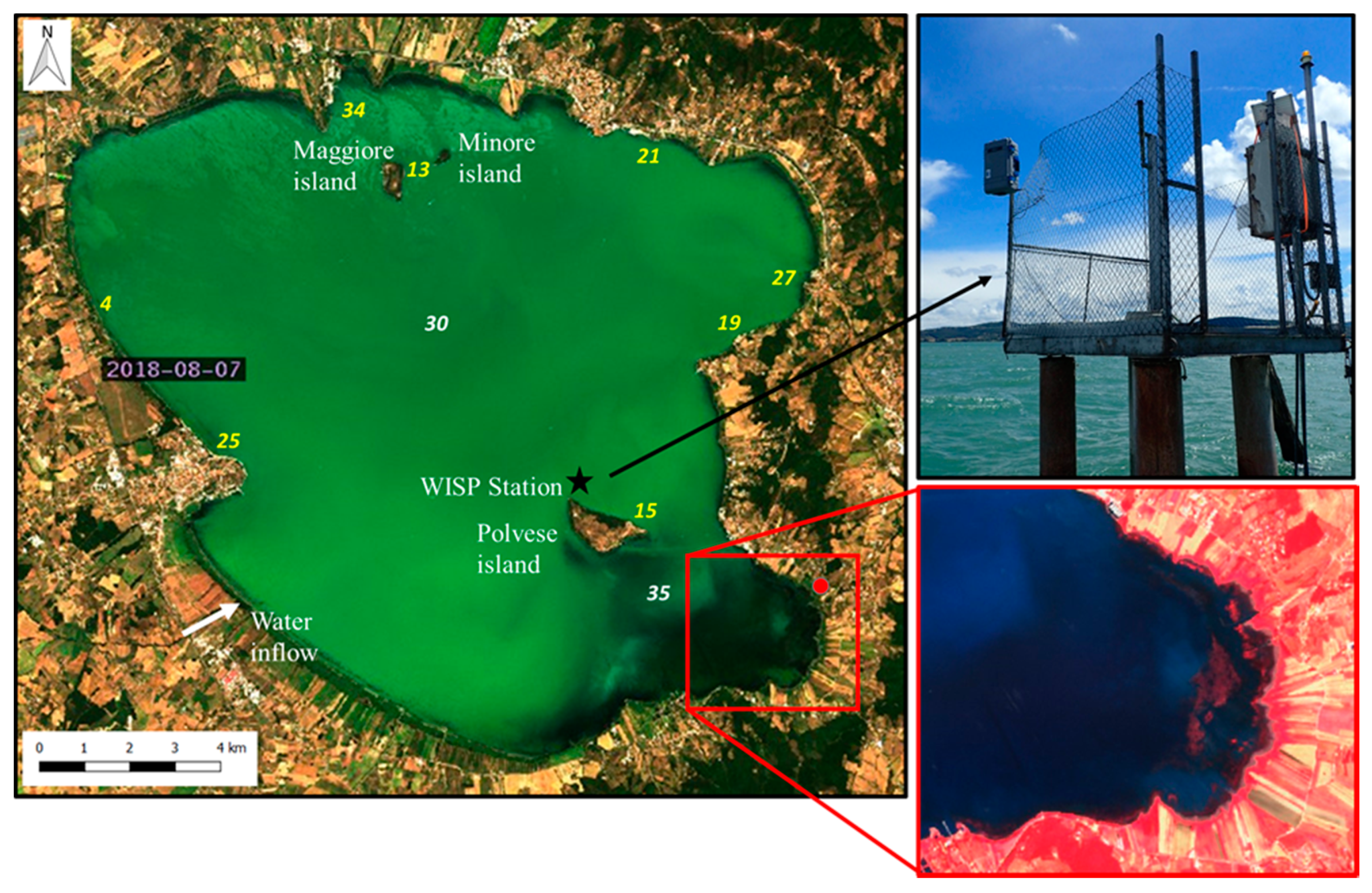
2.1. Study Area

Lake Trasimeno (43°08′ N 12°06′ E; Figure 1), is a post-tectonic, shallow (maximum depth 6 m), turbid (mean Secchi disk depth 1.1 m; mean total suspended matter-TSM 10 g m−3) and eutrophic lake (Chl-a concentration up to 90 mg m−3) in central Italy [38,39] at an average altitude of 257 m a.s.l. It is the fourth largest Italian lake (124 km2) with a diameter of about 11 km and a perimeter of about 53 km, with three small islands (Polvese, Maggiore and Minore islands), and with an open bay colonized by emergent (e.g., Phragmites australis, Typha angustifolia) and submerged (e.g., Potamogeton pectinatus, Chara globularis, Myriophyllum spicatum) macrophytes species in the south-east portion of the lake [40,41] (Figure 1). The lake is closed, without a natural outlet and with small watercourses and runoffs that feed the reservoir, resulting in a long water renewal time (>20 years, [38]). Lake water level is strongly dependent on meteorological conditions (i.e., annual rainfall), and under the current climate change scenario has recorded a significant reduction in water availability [39]. The water column is unstratified, with recurrent sediment resuspension due to wind action [42]. The high nutrient availability favors the occurrence of phytoplankton blooms, including cyanobacteria species (e.g., Cylindrospermopsis raciborskii, Planktothrix agardhii) [43,44]. The main anthropogenic pressures are related to agriculture and livestock practices (arable land cover ~70% of the catchment area, equal to 384 km2), and to tourism (e.g., fishing and bathing) and recreational activities. The lacustrine ecosystem is also an area of exceptional value for flora and fauna richness and species for biodiversity. It is included in a Natural Regional Park and two Natura 2000 sites (IT5210018 and IT5210070).

2.2. WISPstation in Situ Data

The WISPstation [35] radiometers measure the radiance and irradiance in the spectral range of 350–900 nm with a spectral resolution of 4.6 nm (FWHM: full width at half maximum). The WISPstation contains two sets of sensors: one set looks to the NNE and one to the NNW, when installed facing north on the Northern hemisphere (modified from the design of [45]. Each set has a radiance sensor that looks downward to the water surface at an angle of 40 degrees from the vertical (Lup) and a sky looking radiance sensor looking upward at an angle of 40 degrees from the vertical (Lsky). The optimal relative azimuth angle between the sun and one set of sensors is ~135 degrees [46]. The set of sensors that is best oriented with respect to the sun position at any time of the day is automatically selected in the backend WISPcloud. This instrument setup allows the minimization of the amount of sun and sky glint in the measurement. The WISPstation features eight channels: two radiance channels collecting Lup and Lsky in the NNW direction; two radiance channels collecting Lup and Lsky in the NNE direction; two irradiance channels; one unexposed dark radiance channel for evaluation of radiance channel degradation; one unexposed dark irradiance channel for evaluation of the degradation of irradiance channels. All channels are connected to the central spectrometer by means of optical fibers and an optical multiplexer. The advantage of this design is, amongst others, that any variability or degradation of the sensitivity of the spectrometer is compensated in the calculation of remote sensing reflectance. A regular measurement cycle where each channel is measured ten times at an optimal integration time takes usually less than one minute depending on ambient light conditions. The system is calibrated relative to a reference instrument (calibrated in a certified laboratory using a lamp and integrating sphere with NIST traceable calibrations). The WISPstation is watertight and built into a highly climate resistant case. Temperature of the sensor and humidity in the case are registered with every measurement. Data are automatically sent using 3G connectivity to the database (WISPcloud). The instrument can be remotely accessed and, e.g., updated or configured to a specific time interval or measurement frequency. It is autonomously powered by a solar panel and internal large battery.
The WISPstation was located 400 meters from the Polvese island in Lake Trasimeno (Figure 1) and ran from 24 April to 3 October 2018 and collected remote sensing reflectance (Rrs) data every 15 min (4832 acquisitions). Its hyperspectral features allow a simulation of the band setting of satellite data and hence provides valuable reference data. For water quality monitoring purposes, a first estimate of Chl-a was derived through a standard water quality algorithm [47], which make use of a reflectance band ratio at 704 and 672 nm with backscattering derived from the reflectance at 776 nm. The WISPstation derived data of Chl-a concentrations were validated against Chl-a values measured in water samples analyzed by ARPA Umbria (see paragraph “2.5 Ancillary data”). The WISPstation dataset was analyzed for intra and inter-daily variability of water quality properties.

2.3. Satellite Data and Processing

Sentinel-3 satellites (date of launch: A on 16 February 2016; B on April 2018) carry an on board optical sensor (OLCI) acquiring along the visible and near-infrared spectrum (from 400 to 1020 nm) in 21 channels, with a 300 m ground spatial resolution and a daily revisit time. The Sentinel-2 satellites (date of launch: A on 23 June 20157; B on March 2017) carry on board a passive optical sensor (MSI) with 12 spectral bands covering the electromagnetic spectrum in visible to shortwave infrared wavelengths (from 443 to 2201 nm), with a 5-day revisit time and a spatial resolution of 10, 20, or 60 m (depending on the band).
The multi-temporal S3-OLCI and S2-MSI dataset covering Lake Trasimeno for 2018 includes 22 and 20 acquisitions, respectively, based on the availability of clear-sky conditions and low-glint contamination risk. S3-OLCI and S2-MSI images were radiometrically calibrated and converted into Rrs after atmospheric correction performed with Polymer and 6SV-based code, respectively, and have had their accuracy evaluated [32]. Satellite-derived Rrs products were then converted into Chl-a with the bio-optical model implemented in BOMBER [26], parametrized with specific inherent optical properties (SIOPs) of Lake Trasimeno [41]. More detailed information on image processing and match-up between pairs of S3-OLCI and S2-MSI derived products has already been reported [32]. The Chl-a products derived from satellite were compared with in situ WISPstation and water sample data.

2.4. Product Analysis

Chlorophyll-a maps derived from satellite images were analyzed to obtain annual and summer coefficient of variation (CV) values for the lake and then a sub-set of ten regions of interest (ROIs) were selected for spatial-temporal analyses. The CV is the standard deviation divided by the mean providing a standardized measure of dispersion [48]. It useful for comparing among diverse parameters and has been used previously to examine spatial and temporal variation in Chl-a in lake Erie [49,50]. The map of Chl-a concentration CV was analysed to infer zones with the highest spatial variability. From these data the ten ROIs were selected and analysed. The ROIs (of 9 pixels for S3-OLCI, equivalent to 8100 pixels for S2-MSI images) were selected on the basis of the CV of Chl-a concentrations, together with water circulation, presence/absence of macrophyte stands, and the location of the ARPA Umbria in situ monitoring sites (TRS 30 and 35 in Figure 1).
The ecological status of the Lake Trasimeno (category: lake mean depth 3–15 m) was classified in three steps, following the national protocol approach applied in [51]. Firstly, average seasonal concentrations were calculated for spring (1 April–15 May; n = 7 images), spring–summer transition (15 May–15 June; n = 7 images), summer (1 July–31 August; n = 11 images), summer–autumn transition (1 September–1 October; n = 6 images), autumn (1 October–31 November; n = 9 images), and winter (1 January–20 March; n = 2 images). Secondly, these seasonal averages were combined to give an annual average. Thirdly the annual average was classified using the published boundaries [52]: high/good = 4.4 mg m−3; good/moderate = 8.0 mg m−3; moderate/poor = 14.6 mg m−3; poor/bad = 26.7 mg m−3. The advantage of using satellite data with this approach is the possibility to have more than one Chl-a value for each season, to give the average of n images grouped per season, instead of one in situ sampling data per season as required by national regulations (D. Lgs 152/2006). This approach can utilize a more robust dataset to classify water quality on an annual basis, in addition to the obviously greater spatial coverage of the classification.

2.5. Ancillary Data

An annual dataset (2018) for wind velocity and direction (hourly data), solar radiance (data every 30 min), water and air temperature (hourly data) was obtained from Umbria Region Hydrographic Service (data source: data collected continuously in Polvese Island station). In S. Savino station (Magione village; Figure 1) water level relative to hydrometric zero (257.33 m a.s.l.) and precipitation are measured daily (data source: [53]). Atmospheric pressure was taken from the metrological station at S.Maria degli Angeli, Assisi. The wind speed and direction data were used to calculate wind components in an EW and NS direction and wind roses calculated using the R package ‘Openair’ [54,55]. Seven field campaigns were performed by ARPA Umbria to measure Chl-a concentrations closest to the WISPstation (TR 15; Figure 1) on 24 April, 13 and 30 June, 24 July, 16 August, 4 September, and 10 October 2018. Chlorophyll-a was measured spectrophotometrically after extraction in acetone 90% [56]. Cyanobacteria monitoring data (species identification and cell count under the inverted microscope; [57] for eight sampling stations (TRS 4, 13, 15, 19, 21, 25, 27, 34; Figure 1) were also obtained from ARPA Umbria for the period April–September.

2.6. Statistical Analysis

Nonparametric Multiplicative Regression (NPMR) [58] was used to estimate the response of Chl-a to parameters: day of year (DOY), wind velocity and direction (converted to EW and NS wind components and moving averages of 3, 5, and 7 days), solar radiance, atmospheric pressure, lake level, water and air temperature. NPMR can define response surfaces using predictors in a multiplicative rather than in an additive way. This method is progressive in better defining unimodal responses more typical of ecological data than other methods such as multiple regression [58]. It has previously been applied to model tree species distribution [59], the response of lichens to climate change [60], and in time-series analysis [61]. NPMR was applied using the software HyperNiche version 2.3 [62]. The response of Chl-a was estimated using a local mean multiplicative smoothing function with Gaussian weighting. NPMR models were produced by adding predictors stepwise with fit expressed as a cross-validated R2 (xR2) which can be interpreted in a similar way as a measure of fit as a traditional R2. NPMR models were evaluated using a Monte Carlo procedure where abundance was randomised, the procedure rerun, and the proportion of models (p) (with the same number of predictors) with an xR2 greater than or equal to the original model evaluated. The sensitivity, a measure of influence of each parameter included in the NPMR model, was estimated by altering the range of predictors by +/−0.05 (i.e., 5%) with resulting deviations scaled as a proportion of the observed range of the response variable. Therefore, a value of 1 would correspond to change of equal magnitude in response and predictor variables. Sensitivity can be used to evaluate the relative importance of variables included in models because NPMR models are unlike linear regression and have no fixed coefficients or slopes. The order of inclusion of variables in models is less important. Instead of fitting coefficients in NPMR tolerances are fit. These are reported in original units and represent one standard deviation of the Gaussian smoothing function. A trewness smoothed line was fitted to the seasonal pattern in Chl-a using the software DataDesk [63].
In order to identify and aggregate similar patterns in the diurnal response of Chl-a, a hierarchical cluster analysis was carried out using relative Sørensen distance with flexible beta linkage [64]. Discriminant analysis was used to see if environmental variables could correctly classify the different cluster end groups [55,65]. After the removal of autocorrelated variables a total of seven remained for analysis: solar radiance, pressure, rain, water temperature, wind speed, EW and NS wind components.
WISPstation and water sample determined Chl-a were compared by linear regression. While the number of monitoring occasions was only seven, therefore allowing only a limited comparison, the range from <5 to >45 mg m−3 largely represented the seasonal variation in the lake. Reported values included the R2 (coefficient of determination) as well as both the MAE (Mean Absolute Error) and RMSE (Root Mean Squared Error), the former being more easily interpretable and the latter penalizing larger errors ([66]).
Standard deviation was calculated for Chl-a obtained in situ (water sample and WISPstation data) and for concentrations derived from the satellite data. For satellite products, the standard deviation of the Chl-a values was established from the standard deviation of the 3 × 3 pixels of the region of interest. In order to test for overall differences among the regions of interest in Chl-a, the non-parametric Kruskal-Wallis One Way Analysis of Variance on Ranks was applied [67,68].

3. Results and Discussion
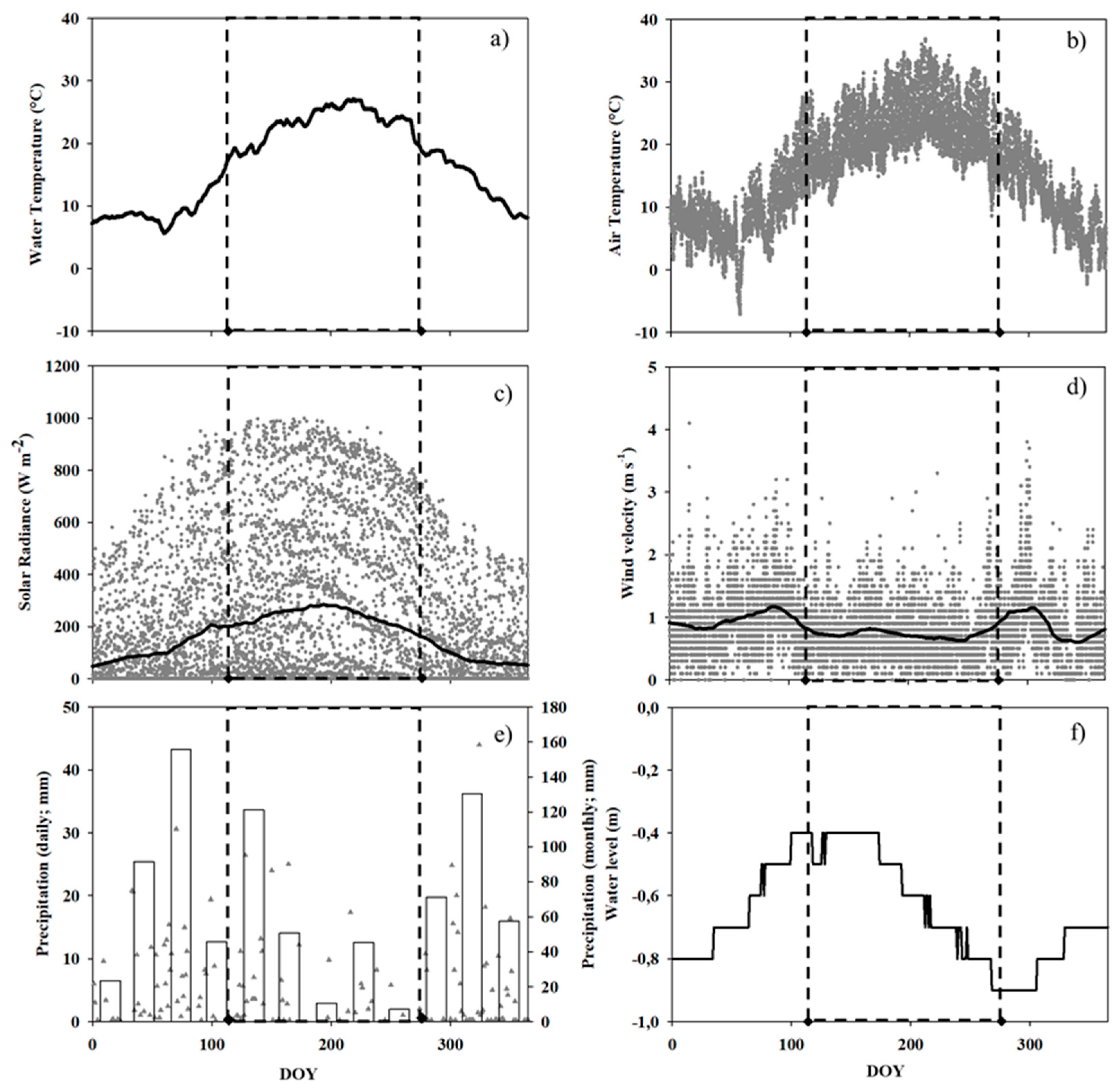
3.1. Ancillary Data

In 2018, the air temperature ranged between −7.1 and 36.8 °C, with a CV of 53%, while water temperature ranged from 5.6 and 27.1 °C with a lower CV (41%) (Figure 2a,b). In the period of WISPstation acquisition, water and air temperature were 23.2 ± 2.7 (average ± standard deviation, here and for the following terms) and 22.3 ± 5.1 °C, respectively (Figure 2a,b). The solar radiance was on average 348 ± 279 W m-2, with summer values of 428 ± 300 W m−2 (Figure 2c). Annually, wind speed was on average 0.8 ± 0.5 m s−1 with a maximum of 4.1 m s−1 (17 January 2018; Figure 2d). From the end of April to October, median wind speed was 0.6 m s−1 (Figure 2d), with a prevalent direction from the North-East. Annual precipitation was 809 mm, and March (156 mm), May (122 mm), and October (130 mm) were the months with the highest rainfall (Figure 2e). In the period of WISPstation acquisition, the rainfall was 29% of the yearly precipitation (Figure 2e). Water level increased from January to May 2018, then decreased until the end of October, due to withdrawal for irrigation purposes (Figure 2f). From November to December the water level increased to the previous values of the spring season (Figure 2f).
Chlorophyll-a concentration derived from the whole WISPstation dataset ranged between 0.5 and 83.9 mg m−3 (median value of 12.5 mg m−3) in the period April–October 2018, with the highest values in August and September (Figure 3). Cyanobacteria were detected from 24 July to 4 September 2018, with the presence of potentially harmful algae (PHA) noted from 6 August 2018 (on average 7% of total Cyanobacteria). The main species identified in terms of number of cells per liter were Cylindrospermopsis raciborskii (on average 56% of PHA), Planktothrix agardhii (26% of PHA), Cuspidothrix issatschenkoi (11% of PHA), and Aphanizomenon sp. (6% of PHA). C. raciborskii was found on 6 August, and C. issatschenkoi on 21 August, while P. agardhii increased from 6 August to 4 September. However, despite these levels of PHA, toxicity tests carried out for bathing water purposes were negative [69].

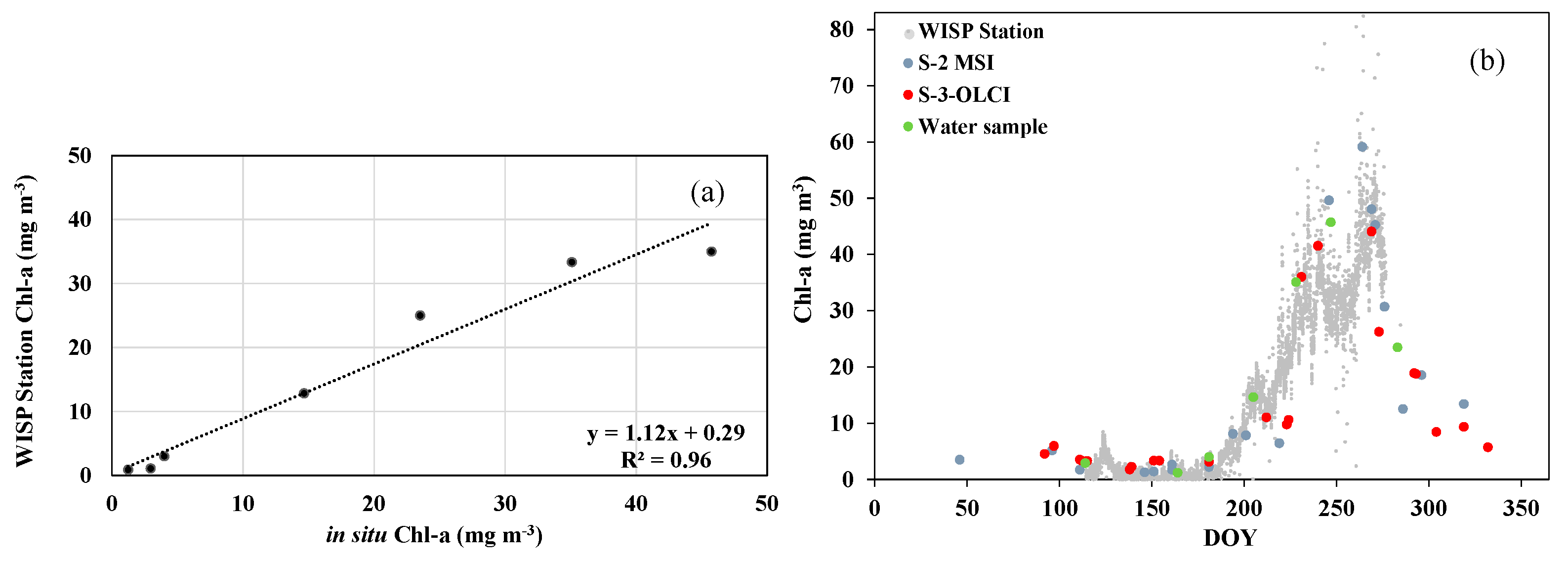
3.2. Validation of Chl-a Products Derived by WISPstation and Satellite Data

Chlorophyll-a concentrations derived from the WISPstation were in good accordance with manual field measurements of Chl-a (MAE = 2.70; RMSE = 23.57 mg m−3; R2 = 0.96; n = 7; Figure 3a), and with Chl-a derived products from S3-OLCI and S2-MSI images (22 and 20 images respectively from 3 × 3 pixels close to the WISPstation; Figure 3b). This validation and cross-comparison of field, satellite, and WISPstation data is an essential step in providing confidence to allow the interchangeable use of the data.

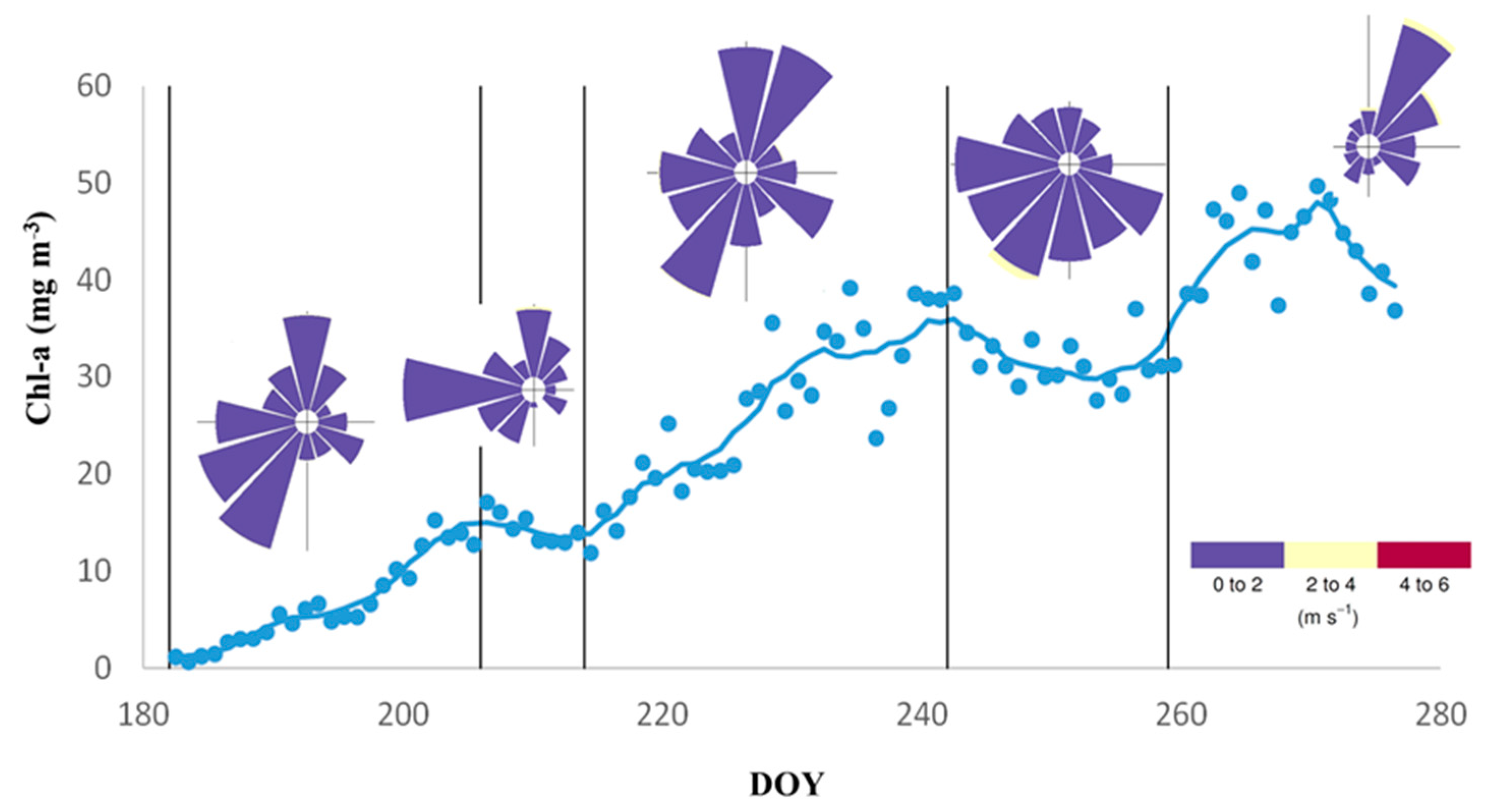
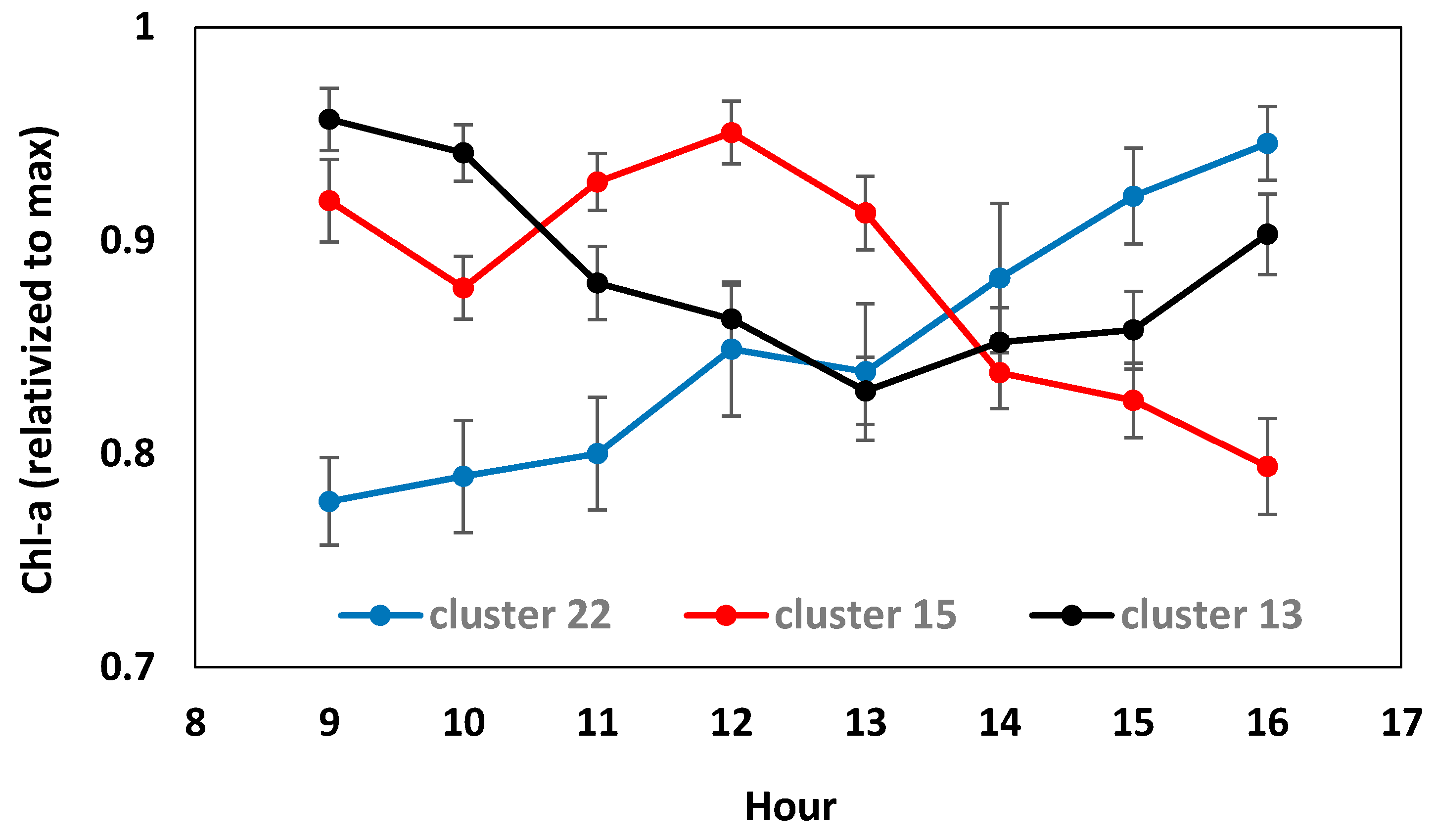
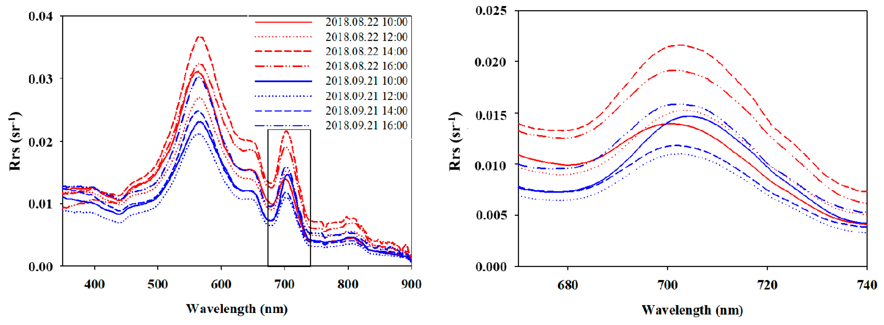
3.3. Intra and Inter-Daily Variation of Chl-a Concentrations from WISPstation Data

The daily evolution of Chl-a derived from the WISPstation, positioned towards the east shore of the lake, showed an increase in phytoplankton abundance starting from 1 July 2018 (DOY 182) (Figure 3b). The maximum values of Chl-a were detected during August (DOY 213) and September (DOY 244), these were also the periods when intra-day variation was at its highest (Figure 3b).
A non-parametric multiplicative regression (NPMR) carried out on the Chl-a data from the WISPstation revealed that the most influential variable was the day of year (sensitivity 0.77) followed by the moving 5-day average of the east–west wind component (sensitivity 0.16) (xR2 = 0.97, p = 0.048) (Table 1). The strong upward growth trend from July was punctuated by periods of stability or decline in Chl-a (indicated by vertical lines in Figure 4). Examining the wind rose for the antecedent period it is apparent that a dominance of westerly winds increase Chl-a, whereas northerly winds cause a decrease (Figure 4).
The significance of day of year reflects the importance of the progressive growth phase of the cyanobacterial bloom. This pattern is common in eutrophic temperate lakes where excessive nutrients, principally phosphorus, lead to the development of cyanobacterial blooms, particularly in low CDOM (Colored Dissolved Organic Matter) high-alkalinity lakes [70,71]. The additional importance of the moving 5-day average of the east–west wind component is likely a result of westerlies concentrating buoyant cyanobacteria on the eastern shore close to where the WISPstation is positioned. Similarially in Lake Erie, the wind component, also with a 5-day lag, was found to be significant in predicting microcystin concentration which was highest following a period of onshore wind and lower during periods of offshore wind [72]. The NPMR model was developed for a limited time-period (April–October 2018). In Lake Trasimeno the timing and slope of increase as well as the date of maximum Chl-a concentration can vary with year, underlining the need for dynamic monitoring that would also provide additional data for more comprehensive model development and validation [44].
While the environmental factors causing variation in Chl-a over days and months were identified above, it may be more challenging to explain the dynamic changes occurring within a day. In order to examine this diurnal variation of Chl-a we initially examined graphs of the hourly variation. It was apparent that while there was no consistent daily pattern, certain patterns were repeated. A cluster analysis of the hourly Chl-a data by day (1 July–3 October) was carried out to group diurnal patterns. Three main groups of daily patterns were reflected: (i) a u-shape (cluster 13, n = 33), (ii) an increase towards 12:00 followed by a decline (cluster 15, n = 20), and (iii) a linear increase (cluster 22, n = 17) (Figure 5). The remaining nine clusters had too few members for interpretation (n ≤ 5). Discriminant analysis was carried out to see if the clusters of daily response shape in Chl-a could be described by environmental variables. Evidence was found that the diurnal patterns in Chl-a for cluster 13 and 15 could be distinguished by the weather factors: solar radiance, pressure, rain, water temperature, wind speed, EW and NS wind components. Discriminant analysis reclassified 70% of cluster 13 and 50% of cluster 15 correctly, in contrast to only 18% of cluster 22. This indicated that the diurnal pattern is likely to be non-random and has a particular response that can, in part, be related to dynamic parameters such as wind speed and direction. Previous work has indicated that variation in physical mixing, temporary stratification, and vertical migration of buoyant cyanobacteria over 2–3 h may be linked to diel variation in Chl-a [73].
For two dates with the maximum daily variation (up to 120%) of Chl-a (22 August and 21 September 2018), the water spectral signatures derived from WISPstation data were examined (Figure 6). In these two dates the intra-daily variation of Chl-a concentration was significantly higher than the 75th percentile of the daily standard deviation of Chl-a. It is evident from the graph the highest peaks of reflectance were measured in the afternoon (at 14:00 on 22 August, and at 16:00 on 21 September; Figure 6). High variation in Chl-a values are to be expected during bloom periods sampled at high frequency. Previous work on diel bloom metabolism has found large differences in Chl-a concentration (up to 75%) along with different patterns of gene expression from samples collected during day and night [74].

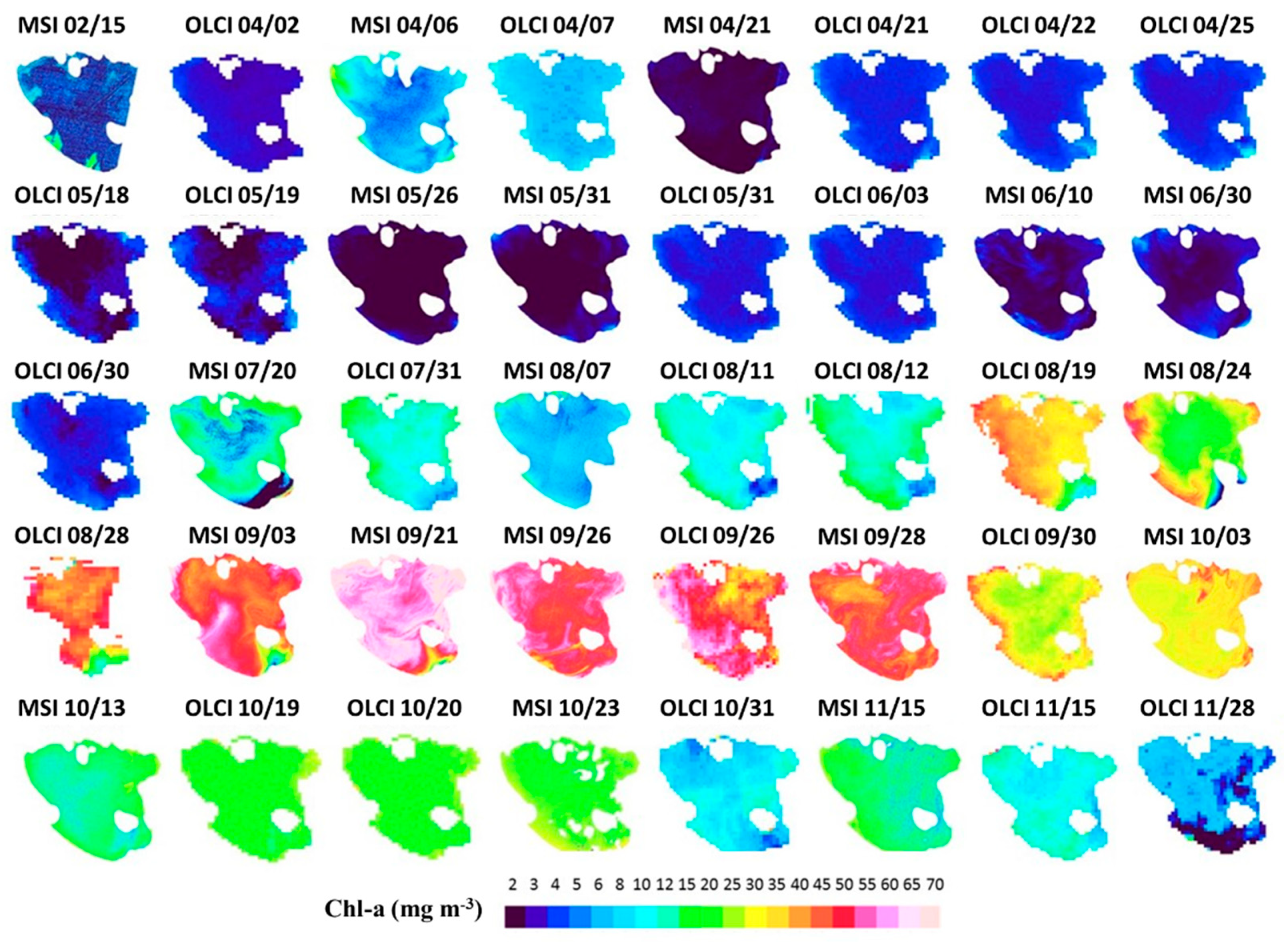
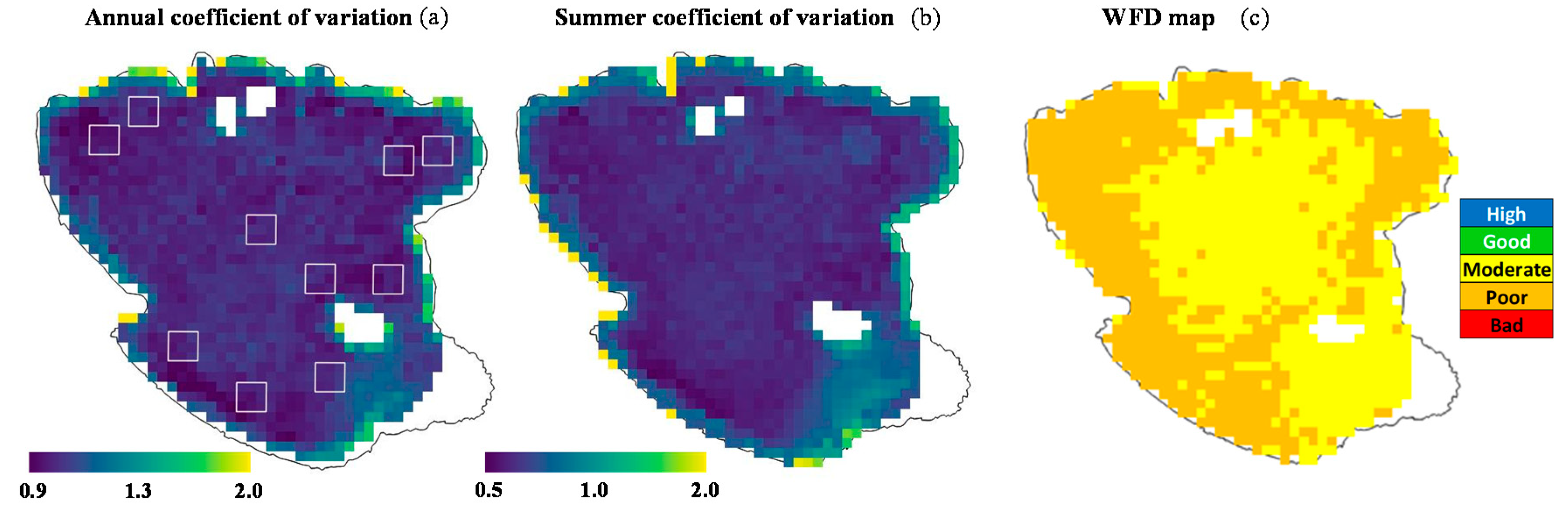
3.4. Temporal and Spatial Distribution of Chl-a Concentration from Satellite Images

Chlorophyll-a maps derived from satellites during 2018 confirmed the seasonal variation in concentration, with highest values in shoreline zones and in the western portion of Lake Trasimeno (Figure 7). Starting from 20 July a substantial increase in Chl-a was visible from the images. On 3 September (DOY 246) a plume of increased Chl-a concentrations is visible emanating from the south-west of the lake close to the water inflow. The following image acquisition (21 September, DOY 264) revealed a more widespread increase in Chl-a and followed a period of persistent southwesterly winds with up to 70 mg Chl-a m−3 detected (Figure 7); this increase was also detected at the WISPstation (DOY 264, Figure 4). High values persisted until the end of September (DOY 271) (Figure 7).
In order to examine if certain zones had persistent problems with elevated concentrations of Chl-a, data from ten regions around the lake were analyzed. When the data were combined over time, no significant difference was found among the regions of interest as tested with a Kruskal-Wallis One Way Analysis of Variance on Ranks. While distinct spatial patterns are clearly visible on given dates (Figure 7) the open nature of this shallow well-mixed lake is such that spatial differences will not remain consistent over time.
Satellite image data used for determining the spatial variation in Chl-a represents an enormous resource with potential, for example, to input into deterministic models improving performance, predictions and understanding [73]. The data allow a much more detailed examination of the temporal and spatial change in Chl-a than would be afforded by traditional manual point sampling. For example, the increase observed from 3 to 21 September appears to be indicative of an increase in nutrient load from the inflow leading to a localized increase in Chl-a which, when followed by a period of westerly winds increases throughout the lake. Though matching nutrient data from the inflow and lake were not available to confirm this, such a rapid increase resulting from supplying an already substantial phytoplankton population with additional nutrients is well demonstrated [75]. Such maps have potential to guide local authorities to areas requiring action to characterize the pollutant source and instigate a restorative programme of measures to achieve good ecological status.
To summarize the spatial variation of Chl-a over time, the coefficient of variation (CV) was calculated for the year 2018 and for the summer period (Figure 8a,b). The annual CV ranged between 0.9 and 2.0, and the map indicated that the shoreline and SE portion of the lake had presumably higher variability of Chl-a concentration (Figure 8a). To understand whether the main influence on the variation was seasonal rather than spatial the same analysis was carried out within the summer period (Figure 8b). This indicated that, although the CV was lower compared to the annual one, the zones with the highest variability were still the shoreline zone and the SE portion of the lake.
The higher variation in the shoreline zone of the lake may be attributed to the more dynamic nature of this zone, as well as the shallower depths and warmer waters promoting phytoplankton growth through higher nutrient release from sediments and increased likelihood of accumulation of buoyant cyanobacteria during periods of onshore wind. Typically, there will be higher sediment resuspension in the shallow littoral, which is a factor of fetch, wind speed, and depth [42]. These factors may also explain the slightly higher variation on the eastern shore often subject to westerly winds (Figure 8b). In the SE portion of the lake the concurrence of shallow water, changing water stability, and the presence of submerged macrophytes can influence both estimation and also the natural variation in phytoplankton abundance and distribution. This area has previously been mapped as having a high vertical density gradient and specific phytoplankton community [76]. High variability in Chl-a concentration can also be due to the role of submerged macrophytes in inhibiting phytoplankton growth during the vegetative period [77]. Moreover, in this portion of the lake changes were historically recorded in terms of colonization by aquatic vegetation and in particular by the reed Phragmites australis. This area of the lake was colonized by reeds in the last century due to the reduction in water level [42,78] but they have recently receded towards the littoral zone, probably as a consequence of die-back [79] and climate change effects [80]. For these reasons, this area was excluded from subsequent analysis to avoid interference.
With the aim of making the results relevant at a policy level the WFD five-class classification scheme (High, Good, Moderate, Poor, and Bad) for Chl-a was applied [37,52]. This resulted in the assignment of Lake Trasimeno to the moderate/poor quality class (Figure 8c). Water quality was slightly better in the pelagic where moderate was assigned, while zones closer to the littoral were classified as poor. Unlike assessments based on point value monitoring, satellite-based assessments have the benefit of providing a spatial estimation of quality. This can guide attempts at restoration to localized areas as well as increasing the understanding of processes and interactions with fundamental lake characteristics such as bathymetry, residence time etc. It is also clear from Figure 8c that those European states that assess their lakes using samples from the shoreline or outlet will have a greater chance of assigning a lower status [81]. Sentinel 2 data has been used on lakes as small as 7 ha, but given the resolution of <60 m the approach can be applied to much smaller lakes [82], and rivers [83].

4. Conclusions

Field based measurements were successfully used to validate Chl-a concentrations results from (i) the high frequency in situ WISPstation and (ii) satellite products from S3-OLCI with S2-MSI. The high frequency dataset from the WISPstation allowed the development of the seasonal bloom in phytoplankton to be tracked at high temporal resolution from July to the end of September 2018. In addition, this enabled other high frequency data for weather to be aligned and included in models. While the influence of ‘day of year’ reflected seasonally driven growth factors as being most important, the influence of wind direction and speed, with a lag of five days, was also significant in determining local concentrations at the WISPstation. Local models such as this could be useful in preparing responses to bloom events in important recreational lakes such as Trasimeno. Also at diurnal scale the variation showed distinct patterns related to environmental variables highlighting the potential of this data to inform deterministic models and track ongoing responses to climate change.
The products obtained from S3-OLCI and S2-MSI were available to map the spatial and seasonal change in Chl-a in Lake Trasimeno. This allowed the patterns in spatial distribution to be seasonally tracked and interpreted alongside the high frequency WISPstation data. The potential influence of localized inflows in contributing to an increase in mid-summer Chl-a concentrations could be visualized and estimations of WFD status realized at fine spatial scale. For monitoring, it also has the potential to surpass current requirements relating to phytoplankton abundance, bloom frequency, and intensity as listed in the WFD. In fact, remote sensing has been recommended for incorporation into the next update of the WFD, which has been criticized as too focused and reductionist, and will allow national authorities to contextualize ecological assessments in a more advanced way both temporally and spatially [84,85,86,87].
While the separate use of satellite or in situ methods have benefits, this study demonstrated the synergistic dividend from combining approaches. Combining S3-OLCI and S2-MSI data yielded over 40 images that were able to identify potential pollution events entering the lake while coupling this with the continuous Chl-a measurements of the WISP and weather stations allowed the dynamics and manifestation of bloom events to be predicted with clear benefits for water management. The integrated and multi-layer approach (combining sources from field, fixed station and multiple satellites) to assessing chlorophyll-a in lakes used here has the benefit of improving confidence and significantly increases the potential for research, monitoring and model development.

Author Contributions

Conceptualization, M.B., M.P., G.F. and C.G.; Data curation, M.B., M.P., G.F. and G.L.; Formal analysis, M.P. and G.F.; Investigation, M.B., M.P., V.D.B. and R.P.; Methodology, M.B., M.L. and C.G.; Supervision, C.G.; Validation, M.B., S.G., R.P. and C.G.; Writing—original draft, M.B., M.P., G.F. and G.L.; Writing—review & editing, M.B., S.G., M.L., S.P., V.D.B. and R.P. All authors have read and agreed to the published version of the manuscript.

Funding

This research received no external funding.

Acknowledgments

This research is part of the H2020 EOMORES (GA n. 730066). We would like to thank the “Cooperativa dei Pescatori del Trasimeno” for the support in field campaigns, and in particular Aurelio Cocchini. Many thanks to Philippe Gröetsch, and Annelies Hommersom for the WISPstation interaction activities and Luca Tamburi, Alessandra Cingolani and Fedra Charavgis from ARPA Umbria for useful discussions, and Luca Nicoletti and Luca Galli from Polvese Center “Climate Change and Biodiversity in Lakes and Wetlands” from ARPA Umbria for collecting water samples. We also thank the Province of Perugia for the availability to use the platform in Polvese Island.

Conflicts of Interest

The authors declare no conflict of interest.

References

  1. Hanjra, M.A.; Qureshi, M.E. Global water crisis and future food security in an era of climate change. Food Policy 2010, 35, 365–377. [Google Scholar] [CrossRef]
  2. Tyler, A.N.; Hunter, P.D.; Spyrakos, E.; Groom, S.; Constantinescu, A.M.; Kitchen, J. Developments in Earth observation for the assessment and monitoring of inland, transitional, coastal and shelf-sea waters. Sci. Total Environ. 2016, 572, 1307–1321. [Google Scholar] [CrossRef] [Green Version]
  3. Ormerod, S.J.; Dobson, M.; Hildrew, A.G.; Townsend, C.R. Multiple stressors in freshwater ecosystems. Freshw. Biol. 2010, 55, 1–4. [Google Scholar] [CrossRef]
  4. Woodward, G.; Perkins, D.M.; Brown, L.E. Climate change and freshwater ecosystems: Impacts across multiple levels of organization. Philos. Trans. R. Soc. B Biol. Sci. 2010, 365, 2093–2106. [Google Scholar] [CrossRef] [PubMed] [Green Version]
  5. Carpenter, S.R.; Stanley, E.H.; Vander Zanden, M.J. State of the World’s Freshwater Ecosystems: Physical, Chemical, and Biological Changes. Annu. Rev. Environ. Resour. 2011, 36, 75–99. [Google Scholar] [CrossRef] [Green Version]
  6. Hestir, E.L.; Brando, V.E.; Bresciani, M.; Giardino, C.; Matta, E.; Villa, P.; Dekker, A.G. Measuring freshwater aquatic ecosystems: The need for a hyperspectral global mapping satellite mission. Remote Sens. Environ. 2015, 167, 181–195. [Google Scholar] [CrossRef] [Green Version]
  7. Klemas, V. Remote sensing of emergent and submerged wetlands: An overview. Int. J. Remote Sens. 2013, 34, 6286–6320. [Google Scholar] [CrossRef]
  8. Kiefer, I.; Odermatt, D.; Anneville, O.; Wüest, A.; Bouffard, D. Application of remote sensing for the optimization of in-situ sampling for monitoring of phytoplankton abundance in a large lake. Sci. Total Environ. 2015, 527–528, 493–506. [Google Scholar] [CrossRef]
  9. Bukata, R.P. Satellite Monitoring of Inland and Coastal Water Quality: Retrospection, Introspection, Future Directions; CRC Press: Boca Raton, FL, USA; Taylor and Francis Group: Abingdon-on-Thames, UK, 2015; ISBN 978-0-8493-3356-9. [Google Scholar]
  10. Schaeffer, B.A.; Schaeffer, K.G.; Keith, D.; Lunetta, R.S.; Conmy, R.; Gould, R.W. Barriers to adopting satellite remote sensing for water quality management. Int. J. Remote Sens. 2013, 34, 7534–7544. [Google Scholar] [CrossRef]
  11. Palmer, S.C.J.; Kutser, T.; Hunter, P.D. Remote sensing of inland waters: Challenges, progress and future directions. Remote Sens. Environ. 2015, 157, 1–8. [Google Scholar] [CrossRef] [Green Version]
  12. Codd, G.A.; Morrison, L.F.; Metcalf, J.S. Cyanobacterial toxins: Risk management for health protection. Toxicol. Appl. Pharmacol. 2005, 203, 264–272. [Google Scholar] [CrossRef] [PubMed]
  13. Jöhnk, K.D.; Huisman, J.; Sharples, J.; Sommeijer, B.; Visser, P.M.; Stroom, J.M. Summer heatwaves promote blooms of harmful cyanobacteria. Glob. Chang. Biol. 2008, 14, 495–512. [Google Scholar] [CrossRef] [Green Version]
  14. Ma, X.; Wang, Y.; Feng, S.; Wang, S. Vertical migration patterns of different phytoplankton species during a summer bloom in Dianchi Lake, China. Environ. Earth Sci. 2015, 74, 3805–3814. [Google Scholar] [CrossRef]
  15. Leal, M.C.; Sá, C.; Nordez, S.; Brotas, V.; Paula, J. Distribution and vertical dynamics of planktonic communities at Sofala Bank, Mozambique. Estuar. Coast. Shelf Sci. 2009, 84, 605–616. [Google Scholar] [CrossRef]
  16. Jindal, R.; Thakur, R.K. Diurnal variations of plankton diversity and physico-chemical characteristics of Rewalsar Wetland, Himachal Pradesh, India. RRST 2013, 5, 4–9. [Google Scholar]
  17. Raymond, J.E.G. Plankton and productivity in the oceans. In Zooplankton; Pergamon Press: Oxford, UK, 1983; p. 824. [Google Scholar]
  18. Ezra, A.G.; Nwankwo, D.I. Composition of phytoplankton algae in Gubi reservoir, Bauchi, Nigeria. J. Aquat. Sci. 2001, 16, 115–118. [Google Scholar] [CrossRef]
  19. Reynolds, C.S. Ecology of Phytoplankton; Cambridge University Press: Cambridge, UK, 2006. [Google Scholar]
  20. Matthews, M.W. Chapter 6—Bio-optical Modeling of Phytoplankton Chlorophyll-a. In Bio-Optical Modeling and Remote Sensing of Inland Waters; Mishra, D.R., Ogashawara, I., Gitelson, A.A., Eds.; Elsevier: Amsterdam, The Netherlands, 2017; pp. 157–188. ISBN 978-0-12-804644-9. [Google Scholar]
  21. Lindell, T.; Pierson, D.; Premazzi, G.; Zilioli, E. Manual for Monitoring European Lakes Using Remote Sensing Techniques EUR Report N. 18665 EN; Office for Official Publications of the European Communities: Luxembourg, 1999. [Google Scholar]
  22. Gilerson, A.A.; Gitelson, A.A.; Zhou, J.; Gurlin, D.; Moses, W.; Ioannou, I.; Ahmed, S.A. Algorithms for remote estimation of chlorophyll-a in coastal and inland waters using red and near infrared bands. Opt. Express 2010, 18, 24109–24125. [Google Scholar] [CrossRef] [Green Version]
  23. Bresciani, M.; Giardino, C.; Lauceri, R.; Matta, E.; Cazzaniga, I.; Pinardi, M.; Lami, A.; Austoni, M.; Viaggiu, E.; Congestri, R.; et al. Earth observation for monitoring and mapping of cyanobacteria blooms. Case studies on five Italian lakes. J. Limnol. 2017, 76, 127–139. [Google Scholar] [CrossRef] [Green Version]
  24. Pinardi, M.; Bresciani, M.; Villa, P.; Cazzaniga, I.; Laini, A.; Tóth, V.; Fadel, A.; Austoni, M.; Lami, A.; Giardino, C. Spatial and temporal dynamics of primary producers in shallow lakes as seen from space: Intra-annual observations from Sentinel-2A. Limnologica 2018, 72, 32–43. [Google Scholar] [CrossRef]
  25. Pierson, D.C.; Strömbeck, N. Estimation of radiance reflectance and the concentrations of optically active substances in Lake Mälaren, Sweden, based on direct and inverse solutions of a simple model. Sci. Total Environ. 2001, 268, 171–188. [Google Scholar] [CrossRef]
  26. Giardino, C.; Candiani, G.; Bresciani, M.; Lee, Z.; Gagliano, S.; Pepe, M. BOMBER: A tool for estimating water quality and bottom properties from remote sensing images. Comput. Geosci. 2012, 45, 313–318. [Google Scholar] [CrossRef]
  27. Gitelson, A.A.; Dall’Olmo, G.; Moses, W.; Rundquist, D.C.; Barrow, T.; Fisher, T.R.; Gurlin, D.; Holz, J. A simple semi-analytical model for remote estimation of chlorophyll-a in turbid waters: Validation. Remote Sens. Environ. 2008, 112, 3582–3593. [Google Scholar] [CrossRef]
  28. Gower, J.F.R.; Doerffer, R.; Borstad, G.A. Interpretation of the 685nm peak in water-leaving radiance spectra in terms of fluorescence, absorption and scattering, and its observation by MERIS. Int. J. Remote Sens. 1999, 20, 1771–1786. [Google Scholar] [CrossRef]
  29. Dörnhöfer, K.; Klinger, P.; Heege, T.; Oppelt, N. Multi-sensor satellite and in situ monitoring of phytoplankton development in a eutrophic-mesotrophic lake. Sci. Total Environ. 2018, 612, 1200–1214. [Google Scholar] [CrossRef] [PubMed]
  30. Nõges, P.; Tuvikene, L. Spatial and annual variability of environmental and phytoplankton indicators in Lake Võrtsjärv: Implications for water quality monitoring. Est. J. Ecol. 2012, 61, 227–246. [Google Scholar] [CrossRef] [Green Version]
  31. Ryu, J.-H.; Han, H.-J.; Cho, S.; Park, Y.-J.; Ahn, Y.-H. Overview of geostationary ocean color imager (GOCI) and GOCI data processing system (GDPS). Ocean Sci. J. 2012, 47, 223–233. [Google Scholar] [CrossRef]
  32. Cazzaniga, I.; Bresciani, M.; Colombo, R.; Della Bella, V.; Padula, R.; Giardino, C. A comparison of Sentinel-3-OLCI and Sentinel-2-MSI-derived Chlorophyll-a maps for two large Italian lakes. Remote Sens. Lett. 2019, 10, 978–987. [Google Scholar] [CrossRef]
  33. Bresciani, M.; Rossini, M.; Morabito, G.; Matta, E.; Pinardi, M.; Cogliati, S.; Julitta, T.; Colombo, R.; Braga, F.; Giardino, C. Analysis of within-and between-day chlorophyll-a dynamics in Mantua Superior Lake, with a continuous spectroradiometric measurement. Mar. Freshw. Res. 2013, 64, 303–316. [Google Scholar] [CrossRef]
  34. Kwon, Y.S.; Jang, E.; Im, J.; Baek, S.H.; Park, Y.; Cho, K.H. Developing data-driven models for quantifying Cochlodinium polykrikoides using the Geostationary Ocean Color Imager (GOCI). Int. J. Remote Sens. 2018, 39, 68–83. [Google Scholar] [CrossRef]
  35. Peters, S.; Laanen, M.; Groetsch, P.; Ghezehegn, S.; Poser, K.; Hommersom, A.; De Reus, E.; Spaias, L. WISPstation: A new autonomous above water radiometer system. In Proceedings of the Ocean Optics XXIV Conference, Dubrovnik, Croatia, 7–12 October 2018. [Google Scholar]
  36. Council of the European Communities. Directive 2000/60/EC of the European Parliament and of the Council of 23 October 2000 Establishing a Framework for Community Action in the Field of Water Policy. Off. J. Eur. Commun. 2000, 22, 2000. [Google Scholar]
  37. Council of the European Communities. Commission Decision of 20 September 2013 establishing, pursuant to Directive 2000/60/EC of the European Parliament and of the Council, the values of the Member State monitoring system classifications as a result of the intercalibration exercise and repealing Decision 2008/915/EC. Off. J. Eur. Commun. 2013, 480, 1–47. [Google Scholar]
  38. Ludovisi, A.; Poletti, A. Use of thermodynamic indices as ecological indicators of the development state of lake ecosystems. 1. Entropy production indices. Ecol. Model. 2003, 159, 203–222. [Google Scholar] [CrossRef]
  39. Giardino, C.; Bresciani, M.; Villa, P.; Martinelli, A. Application of Remote Sensing in Water Resource Management: The Case Study of Lake Trasimeno, Italy. Water Resour. Manag. 2010, 24, 3885–3899. [Google Scholar] [CrossRef]
  40. Landucci, F.; Gigante, D.; Venanzoni, R. An application of the Cocktail method for the classification of the hydrophytic vegetation at Lake Trasimeno (Central Italy). Fitosociologia 2011, 48, 3–22. [Google Scholar]
  41. Giardino, C.; Bresciani, M.; Valentini, E.; Gasperini, L.; Bolpagni, R.; Brando, V.E. Airborne hyperspectral data to assess suspended particulate matter and aquatic vegetation in a shallow and turbid lake. Remote Sens. Environ. 2015, 157, 48–57. [Google Scholar] [CrossRef]
  42. Ludovisi, A.; Gaino, E. Meteorological and water quality changes in Lake Trasimeno (Umbria, Italy) during the last fifty years. J. Limnol. 2010, 69, 174–188. [Google Scholar] [CrossRef] [Green Version]
  43. Salmaso, N. Long-term phytoplankton community changes in a deep subalpine lake: Responses to nutrient availability and climatic fluctuations. Freshw. Biol. 2010, 55, 825–846. [Google Scholar] [CrossRef]
  44. Bresciani, M.; Giardino, C.; Boschetti, L. Multi-temporal assessment of bio-physical parameters in lakes Garda and Trasimeno from MODIS and MERIS. Ital. J. Remote Sens./Rivista Italiana Di Telerilevamento 2011, 43, 49–62. [Google Scholar]
  45. Wernand, M.R. Guidelines for (Ship-Borne) Auto-Monitoring of Coastal and Ocean Colour. In Proceedings of the Ocean Optics XVI, Santa Fe, NM, USA, 8–22 November 2002; Volume 13. [Google Scholar]
  46. Mobley, C.D. Estimation of the remote-sensing reflectance from above-surface measurements. Appl. Opt. 1999, 38, 7442–7455. [Google Scholar] [CrossRef]
  47. Gons, H.J. Optical teledetection of chlorophyll a in turbid inland waters. Environ. Sci. Technol. 1999, 33, 1127–1132. [Google Scholar] [CrossRef]
  48. Friedemann, G.; Schellenberg, J. Goeveg: Functions for Community Data and Ordinations; Comprehensive R Archive Network. 2018. Available online: https://cran.r-project.org/web/packages/goeveg (accessed on 9 September 2019).
  49. Fang, S.; Del Giudice, D.; Scavia, D.; Binding, C.E.; Bridgeman, T.B.; Chaffin, J.D.; Evans, M.A.; Guinness, J.; Johengen, T.H.; Obenour, D.R. A space-time geostatistical model for probabilistic estimation of harmful algal bloom biomass and areal extent. Sci. Total Environ. 2019, 695, 133776. [Google Scholar] [CrossRef] [PubMed]
  50. Brunori, C.; Morabito, R.; Ipolyi, I.; Pellegrino, C.; Ricci, M.; Bercaru, O.; Ulberth, F.; Sahuquillo, A.; Rosenberg, E.; Madrid, Y. The SWIFT-WFD Proficiency Testing campaigns in support of implementing the EU Water Framework Directive. TrAC Trends Anal. Chem. 2007, 26, 993–1004. [Google Scholar] [CrossRef]
  51. Bresciani, M.; Stroppiana, D.; Odermatt, D.; Morabito, G.; Giardino, C. Assessing remotely sensed chlorophyll-a for the implementation of the Water Framework Directive in European perialpine lakes. Sci. Total Environ. 2011, 409, 3083–3091. [Google Scholar] [CrossRef] [PubMed] [Green Version]
  52. Wolfram, G.; Argillier, C.; de Bortoli, J.; Buzzi, F.; Dalmiglio, A.; Dokulil, M.T.; Hoehn, E.; Marchetto, A.; Martinez, P.-J.; Morabito, G.; et al. Reference conditions and WFD compliant class boundaries for phytoplankton biomass and chlorophyll-a in Alpine lakes. Hydrobiologia 2009, 633, 45–58. [Google Scholar] [CrossRef] [Green Version]
  53. Umbrian Regional Hydrographic Service. Available online: https://annali.regione.umbria.it/# (accessed on 9 September 2019).
  54. Carslaw, D.C.; Ropkins, K. Openair—An R package for air quality data analysis. Environ. Model. Softw. 2012, 27, 52–61. [Google Scholar] [CrossRef]
  55. R Core Team. R: A Language and Environment for Statistical Computing; R Foundation for Statistical Computing: Vienna, Austria, 2019. [Google Scholar]
  56. IRSA-CNR; APAT. Metodi Analitici per le Acque. Manuali e Linee Guida. 29/2003; Agenzia per la protezione dell’ambiente e per i servizi tecnici: Romo, Italy, 2003; Volume 9020. [Google Scholar]
  57. Utermöhl, H. Zur vervollkommnung der quantitativen phytoplankton-methodik. Internationale Vereinigung für theoretische und angewandte Limnologie: Mitteilungen 1958, 9, 1–38. [Google Scholar]
  58. McCune, B. Nonparametric Multiplicative Regression for Habitat Modeling; Oregon State University: Corvallis, OR, USA, 2006. [Google Scholar]
  59. Yost, A.C. Probabilistic modeling and mapping of plant indicator species in a Northeast Oregon industrial forest, USA. Ecol. Indic. 2008, 8, 46–56. [Google Scholar] [CrossRef]
  60. Ellis, C.J.; Coppins, B.J.; Dawson, T.P.; Seaward, M.R. Response of British lichens to climate change scenarios: Trends and uncertainties in the projected impact for contrasting biogeographic groups. Biol. Conserv. 2007, 140, 217–235. [Google Scholar] [CrossRef]
  61. Nicolaou, N.; Constandinou, T.G. A Nonlinear Causality Estimator Based on Non-Parametric Multiplicative Regression. Front. Neuroinform. 2016, 10, 9. [Google Scholar] [CrossRef] [Green Version]
  62. McCune, B.; Mefford, M.J. HyperNiche. Nonparametric Multiplicative Habitat Modeling; MjM Software: Gleneden Beach, OR, USA, 2009. [Google Scholar]
  63. Velleman, P.F. Data Desk: Handbook, Volume 1 (1); Data Description, Inc.: New York, NY, USA, 1989. [Google Scholar]
  64. McCune, B.; Mefford, M.J. PC-ORD. Multivariate Analysis of Ecological Data; MjM Software: Gleneden Beach, OR, USA, 2016. [Google Scholar]
  65. Ripley, B.; Venables, B.; Bates, D.M.; Hornik, K.; Gebhardt, A.; Firth, D.; Ripley, M.B. Package MASS: Support Functions and Datasets for Venables and Ripley’s MASS. Comprehensive R Archive Network, 2019. Available online: https://cran.r-project.org/web/packages/MASS (accessed on 9 September 2019).
  66. Chai, T.; Draxler, R.R. Root mean square error (RMSE) or mean absolute error (MAE)—Arguments against avoiding RMSE in the literature. Geosci. Model Dev. 2014, 7, 1247–1250. [Google Scholar] [CrossRef] [Green Version]
  67. Systat. SigmaPlot for Windows, Version 11.0; Systat Software: Chicago, IL, USA, 2008. [Google Scholar]
  68. Daniel, W.W. Kruskal–Wallis one-way analysis of variance by ranks. Appl. Nonparametric Stat. 1990, 226–234. [Google Scholar]
  69. Charavgis, F.; Cingolani, A.; Di Brizio, M.; Tozzi, G.; Rinaldi, E.; Stranieri, P. Qualita’ delle acque di balneazione dei laghi Umbri; ARPA: Umbria, Italty, 2018. [Google Scholar]
  70. Carvalho, L.; Miller, C.A.; Scott, E.M.; Codd, G.A.; Davies, P.S.; Tyler, A.N. Cyanobacterial blooms: Statistical models describing risk factors for national-scale lake assessment and lake management. Sci. Total Environ. 2011, 409, 5353–5358. [Google Scholar] [CrossRef] [PubMed] [Green Version]
  71. Bonilla, S.; Aubriot, L.; Soares, M.C.S.; González-Piana, M.; Fabre, A.; Huszar, V.L.M.; Lürling, M.; Antoniades, D.; Padisák, J.; Kruk, C. What drives the distribution of the bloom-forming cyanobacteria Planktothrix agardhii and Cylindrospermopsis raciborskii? FEMS Microbiol. Ecol. 2012, 79, 594–607. [Google Scholar] [CrossRef] [PubMed]
  72. Francy, D.S.; Brady, A.M.G.; Ecker, C.D.; Graham, J.L.; Stelzer, E.A.; Struffolino, P.; Dwyer, D.F.; Loftin, K.A. Estimating microcystin levels at recreational sites in western Lake Erie and Ohio. Harmful Algae 2016, 58, 23–34. [Google Scholar] [CrossRef]
  73. Hamilton, D.P.; Carey, C.C.; Arvola, L.; Arzberger, P.; Brewer, C.; Cole, J.J.; Gaiser, E.; Hanson, P.C.; Ibelings, B.W.; Jennings, E. A Global Lake Ecological Observatory Network (GLEON) for synthesising high-frequency sensor data for validation of deterministic ecological models. Inland Waters 2015, 5, 49–56. [Google Scholar] [CrossRef] [Green Version]
  74. Davenport, E.J.; Neudeck, M.J.; Matson, P.G.; Bullerjahn, G.S.; Davis, T.W.; Wilhelm, S.W.; Denny, M.K.; Krausfeldt, L.E.; Stough, J.M.A.; Meyer, K.A. Metatranscriptomic analyses of diel metabolic functions during a Microcystis bloom in western Lake Erie (USA). Front. Microbiol. 2019, 10, 2081. [Google Scholar] [CrossRef]
  75. Irvine, K.; Allott, N.; deEyto, E.; Free, G.; White, J.; Caroni, R.; Kennelly, C.; Keaney, J.; Lennon, C.; Kemp, A.; et al. Ecological Assessment of Irish Lakes; Environmental Protection Agency: Wexford, Ireland, 2001; Volume 1, ISBN 1-84095-059-5. [Google Scholar]
  76. Ludovisi, A.; Minozzo, M.; Pandolfi, P.; Taticchi, M.I. Modelling the horizontal spatial structure of planktonic community in Lake Trasimeno (Umbria, Italy) using multivariate geostatistical methods. Ecol. Model. 2005, 181, 247–262. [Google Scholar] [CrossRef]
  77. Van Donk, E.; van de Bund, W.J. Impact of submerged macrophytes including charophytes on phyto-and zooplankton communities: Allelopathy versus other mechanisms. Aquat. Bot. 2002, 72, 261–274. [Google Scholar] [CrossRef]
  78. Granetti, B. La flora e la vegetazione del Lago Trasimeno. Parte I: La vegetazione litoranea. Rivista di Idrobiol 1965, 4, 115–153. [Google Scholar]
  79. Gigante, D.; Venanzoni, R.; Zuccarello, V. Reed die-back in southern Europe? A case study from Central Italy. C. R. Biol. 2011, 334, 327–336. [Google Scholar] [CrossRef]
  80. Pareeth, S.; Bresciani, M.; Buzzi, F.; Leoni, B.; Lepori, F.; Ludovisi, A.; Morabito, G.; Adrian, R.; Neteler, M.; Salmaso, N. Warming trends of perialpine lakes from homogenised time series of historical satellite and in-situ data. Sci. Total Environ. 2017, 578, 417–426. [Google Scholar] [CrossRef] [PubMed]
  81. Phillips, G.; Free, G.; Karottki, I.; Laplace-Treyture, C.; Maileht, K.; Mischke, U.; Ott, I.; Pasztaleniec, A.; Portielje, R.; Søndergaard, M.; et al. Water Framework Directive Intercalibration Technical Report; European Commission: Ispra, Italy, 2014; ISBN 978-92-79-35463-2. [Google Scholar]
  82. Toming, K.; Kutser, T.; Laas, A.; Sepp, M.; Paavel, B.; Nõges, T. First Experiences in Mapping Lake Water Quality Parameters with Sentinel-2 MSI Imagery. Remote Sens. 2016, 8, 640. [Google Scholar] [CrossRef] [Green Version]
  83. Kuhn, C.; de Matos Valerio, A.; Ward, N.; Loken, L.; Sawakuchi, H.O.; Kampel, M.; Richey, J.; Stadler, P.; Crawford, J.; Striegl, R.; et al. Performance of Landsat-8 and Sentinel-2 surface reflectance products for river remote sensing retrievals of chlorophyll-a and turbidity. Remote Sens. Environ. 2019, 224, 104–118. [Google Scholar] [CrossRef] [Green Version]
  84. Carvalho, L.; Mackay, E.B.; Cardoso, A.C.; Baattrup-Pedersen, A.; Birk, S.; Blackstock, K.L.; Borics, G.; Borja, A.; Feld, C.K.; Ferreira, M.T. Protecting and restoring Europe’s waters: An analysis of the future development needs of the Water Framework Directive. Sci. Total Environ. 2019, 658, 1228–1238. [Google Scholar] [CrossRef]
  85. Kelly, M.G.; King, L.L.; Yallop, M.L. As trees walking: The pros and cons of partial sight in the analysis of stream biofilms. Plant Ecol. Evol. 2019, 152, 120–130. [Google Scholar] [CrossRef]
  86. Papathanasopoulou, E.; Simis, S.; Alikas, K.; Ansper, A.; Anttila, S.; Attila, J. Satellite-Assisted Monitoring of Water Quality to Support the Implementation of the Water Framework Directive; EOMORES White Paper; European Union’s Horizon 2020 Project; European Commission: Brussels, Belgium, 2020. [Google Scholar] [CrossRef]
  87. Voulvoulis, N.; Arpon, K.D.; Giakoumis, T. The EU Water Framework Directive: From great expectations to problems with implementation. Sci. Total Environ. 2017, 575, 358–366. [Google Scholar] [CrossRef] [Green Version]
Figure 1. Maps of the Lake Trasimeno from Sentinel-2A (7 August 2018) image in true and false color, showing the WISPstation position (black star) and the bay colonized by aquatic vegetation (red box). The ARPA Umbria stations for WFD (sites TRS30 and 35 in white), bathing (sites TRS 4, 13, 15, 19, 21, 25, 27, 34 in yellow), and water level and precipitation monitoring (S. Savino station; red point) are also reported. Picture of the platform with the WISPstation (on the right).
Water 12 00284 g001
Figure 2. (a) Hourly data of water temperature; (b) hourly data of air temperature; (c) solar radiance; (d) wind velocity; (e) daily and monthly precipitation; (f) daily water level for the Lake Trasimeno in 2018. The black dashed rectangle highlights the time of WISPstation acquisition (from 24 April to 3 October).
Water 12 00284 g002
Figure 3. (a) Scatterplot of chlorophyll-a (Chl-a) data obtained from WISPstation and in situ water sampling. (b) Time series of Chl-a obtained from WISPstation, S3-OLCI and S2-MSI data, and in situ water sampling for Polvese island in 2018. DOY = Day of Year. Two images were not used as they were partially masked by clouds.
Water 12 00284 g003
Figure 4. Chlorophyll-a concentration obtained from WISPstation data (in light blue) from 1 July to 3 October 2018. Trewness smoothed line fit to data [63]. Wind roses (frequency of counts by wind direction) were calculated for the periods indicated by the vertical lines. DOY = Day of Year.
Water 12 00284 g004
Figure 5. Average hourly (UTC time) Chlorophyll-a (Chl-a), relativized to maximum value per day, for cluster 22 (increasing), cluster 15 (an increase towards 12:00 followed by a decline), and cluster 13 (u-shape). Error bars represent standard error.
Water 12 00284 g005
Figure 6. Daily variation (UTC time) in water spectral signatures (remote sensing reflectance, Rrs) from WISPstation data on the 22 August (red lines) and the 21 September (blue lines) 2018. On the right enlarged detail from the box showing reflectance spectra between 670 and 740 nm and differences in hourly reflectance peak.
Water 12 00284 g006
Figure 7. Chlorophyll-a maps of Lake Trasimeno in 2018 from Sentinel-3 OLCI and Sentinel-2 MSI. Only 40 of 42 images are presented, as two S2-MSI images on 28 February and 13 July 2018 had less than 30% of lake surface available for processing.
Water 12 00284 g007
Figure 8. (a) Map of the coefficient of variation for chlorophyll-a concentration for the year 2018 (40 images); and (b) for the summer (11 images) and (c) maps of Water Framework Directive (WFD) classification of Lake Trasimeno based on chlorophyll-a concentration. Squares indicate the regions of interest selected for spatial analysis. White areas are masked zones for macrophytes presence.
Water 12 00284 g008
Table 1. Results of NPMR (Non-Parametric Multiplicative Regression) model for Chlorophyll-a (Chl-a; n = 163, 24 April–3 October). xR2 = cross-validated R2; Ave. size = Average neighborhood size; Tol. = Tolerance; Sen. = Sensitivity. 5 Day EW = the moving 5-day average of the east-west wind component.
VariablexR²Ave. SizeVariable 1Tol.Sen.Variable 2Tol.Sen.
Chlorophyll-a0.978.15Day of Year6.40.775 Day EW0.150.16

