Is Clustering Time-Series Water Depth Useful? An Exploratory Study for Flooding Detection in Urban Drainage Systems


1
Department of Civil and Environmental Engineering, University of Utah, 201 Presidents Circle, Salt Lake City, UT 84112, USA
2
Geography Department, University of Utah, 201 Presidents Circle, Salt Lake City, UT 84112, USA
3
Unit of Environmental Engineering, University of Innsbruck, Innrain 52, 6020 Innsbruck, Austria
*
Author to whom correspondence should be addressed.
Water 2020, 12(9), 2433; https://0-doi-org.brum.beds.ac.uk/10.3390/w12092433
Submission received: 26 July 2020
/
Revised: 21 August 2020
/
Accepted: 25 August 2020
/
Published: 30 August 2020
(This article belongs to the Special Issue Smart Urban Water Networks)
Abstract
:As sensor measurements emerge in urban water systems, data-driven unsupervised machine learning algorithms have drawn tremendous interest in event detection and hydraulic water level and flow prediction recently. However, most of them are applied in water distribution systems and few studies consider using unsupervised cluster analysis to group the time-series hydraulic-hydrologic data in stormwater urban drainage systems. To improve the understanding of how cluster analysis contributes to flooding location detection, this study compared the performance of K-means clustering, agglomerative clustering, and spectral clustering in uncovering time-series water depth dissimilarity. In this work, the water depth datasets are simulated by an urban drainage model and then formatted for a clustering problem. Three standard performance evaluation metrics, namely the silhouette coefficient index, Calinski–Harabasz index, and Davies–Bouldin index are employed to assess the clustering performance in flooding detection under various storms. The results show that silhouette coefficient index and Davies–Bouldin index are more suitable for assessing the performance of K-means and agglomerative clustering, while the Calinski–Harabasz index only works for spectral clustering, indicating these clustering algorithms are metric-dependent flooding indicators. The results also reveal that the agglomerative clustering performs better in detecting short-duration events while K-means and spectral clustering behave better in detecting long-duration floods. The findings of these investigations can be employed in urban stormwater flood detection at the specific junction-level sites by using the occurrence of anomalous changes in water level of correlated clusters as flood early warning for the local neighborhoods.
1. Introduction
Urban drainage systems (UDSs) are the infrastructures constructed to provide conveyance ability and storage capability for drainage overflow mitigation, surface inundation reduction, and pollutant removal. However, the existing UDSs, whose functionality can only serve for a limited number of years, might degrade and even deteriorate as time goes by [1]. In recent years, retrofitting the traditional UDSs with water-level sensors, velocity meters, and flow sensors has been widely adopted as an adaptive and cost-effective solution for flooding challenges [2,3]. The deployed sensors can measure the water quantity and quality data in a real-time way, which now makes it feasible for decision-makers and stakeholders to foresee the potential flood events and locate the vulnerable sites, which supports decision making. The need to understand the emerging data is crucial for forecasting flash floods, reducing sewer overflows, and detecting flooded sites [4,5,6]. Interpreting big water data for flood detection is attracting increasing attention from researchers [7,8,9,10] and can be employed to reduce potential flood damages.
In the last decade, many scholars have introduced several machine learning techniques to investigate the available water resources and hydrological datasets [11,12,13]. The major machine learning algorithms employed for flood detection are support vector machines [14,15], neuro-fuzzy [16], adaptive neuro-fuzzy inference systems, multilayer perceptron [17], random forest [18], and classification and regression trees [19]. Bowes et al. compared long short-term memory and recurrent neural networks by using a time-series of groundwater table data in the city of Norfolk, Virginia [20]. They explained that a long short-term memory neural network is better than the recurrent neural network in predicting groundwater level, but takes about three times longer to train the model. Hu et al. applied a boosted decision regression tree to detect drainage floods with over 90% accuracy in combined sewer systems of Detroit city, Michigan [21]. Li proposed a data-driven fuzzy neural method for reducing downstream urban flooding volume and showed that with an enhanced genetic algorithm optimization the regression deviations could be reduced from 0.22 to 0.07 [22]. However, the majority of these studies have focused on supervised learning (i.e., when a known outcome is used to train the model), and unsupervised machine learning algorithms (UMLA) are not commonly used in stormwater UDSs.
Clustering algorithms are a data-driven technology without considering the classification standard of different risk levels and thereby provide more objective and reasonable results [23]. Therefore, cluster analysis, one of the key unsupervised machine learning methods, has been applied in many fields, including pattern recognition, image analysis, data compression, and anomaly detection [24]. However, its applicability in urban flood detecting is yet to be fully investigated. In general, cluster analysis is based on identifying similarities between observations. If a water quantity or quality event happens in the water system, these observations are likely to be highly dissimilar to other observations [25]. The increment in dissimilarity would lead to these observations being considered as outliers, and thus detected as anomalies. Although cluster analysis has been extensively discussed in municipal topology classification and water distribution network simplification [26,27], the ability of UMLA methods to group time-series data at UDSs is still unknown, and the most appropriate methods to assess these algorithms are unclear. Keogh and Lin concluded that clustering time-series data is meaningless, but this argument does not cover the similarity-based clustering algorithms such as K-means and agglomerative clustering [28]. In contrast, Chen demonstrated that similarity-based cluster analysis could be successfully applied to sequence datasets by using different distance measures [29,30]. Wu et al. adopted the clustering algorithm [24], developed by Rodriguez and Laio [31], to detect the short-duration pipe burst with a 0.61% false positive in water distribution systems. Xing and Sela selected SCI (silhouette coefficient index) and CHI (Calinski–Harabasz index) as the metrics to evaluate K-mean clustering (KC) performance in clustering time-series water pressure data and they finally identified the number of clusters for the pressure sensor placement [32]. However, it was unclear why they chose these two indexes as the UMLA performance metrics. Previous studies from the computer science field have demonstrated the differences and similarities among the popular performance evaluation indices such as SCI, CHI, and DBI (Davies–Bouldin index) [33,34,35]. However, there is no systematic study of how these apply to time-series data from UDSs.
Floods are one of the most hazardous natural events in the world. The short response time against flood events makes them challenging for the hydrologists, and as a result, floods cause loss of life, economics, infrastructure, and property worldwide annually [36,37]. Researchers are trying to promote flooding indicators to identify flooding locations ahead of extreme storm events. There are several hydro-meteorological indicators, such as temperature, humidity, and precipitation, which are related to flood events. The most widely used indicator is hydraulic water level since it can be efficiently and continuously monitored and forecasted to facilitate floods early detection and warning [38]. To efficiently capture the flood events, the flooding water level should be well investigated.
In this study, clustering algorithms, including KC, agglomerative (AC), and spectral clustering (SC), are applied for the urban flood tracking. A storm water management model (SWMM) is established to represent the real-world stormwater urban drainage systems, located in Sugar House neighborhood, Salt Lake City, UT, USA. Three evaluation indices are used to test the performance analysis of the clustering algorithms, namely SCI, CHI, and DBI. The whole research is driven by the hypothesis that the clustering of time-series water level data has the potential to facilitate flooding location detection in the Sugar House Area. The investigations provide answers to various inter-related research questions: (1) What is the performance of different clustering algorithms in capturing the floods? (2) Which metrics are the most suitable for assessing cluster model performance based on hydraulic-hydrologic data in UDSs? (3) Which features of flood time-series data (length, volume and variability) are the most influential for flooding detection, and how does the choice of data feature affect the clustering performance in localizing the flooding sites?
To answer these questions, it is necessary to explore how UMLA groups time-series water depth data, and which assessment score can best represent UMLA performance. However, challenges to implement UMLA with time-series data still exist. Firstly, it is essential to re-format the time-series water depth datasets to make them suitable for clustering problem. This difficulty is associated with the second research question above since the features of datasets determine how we re-structure the data frame [39]. Secondly, the connection between the number of clusters and the clustering model performance is another obstacle. As it is still unknown how to correlate clustering performance and the number of clusters in the stormwater systems, it is necessary to build such a theoretical relationship for a practical application like the flooding detection herein [40]. Therefore, the study aims to improve the understanding of how UMLA facilitates detecting hydraulic anomaly according to the characteristics of water depth datasets in urban drainage networks.
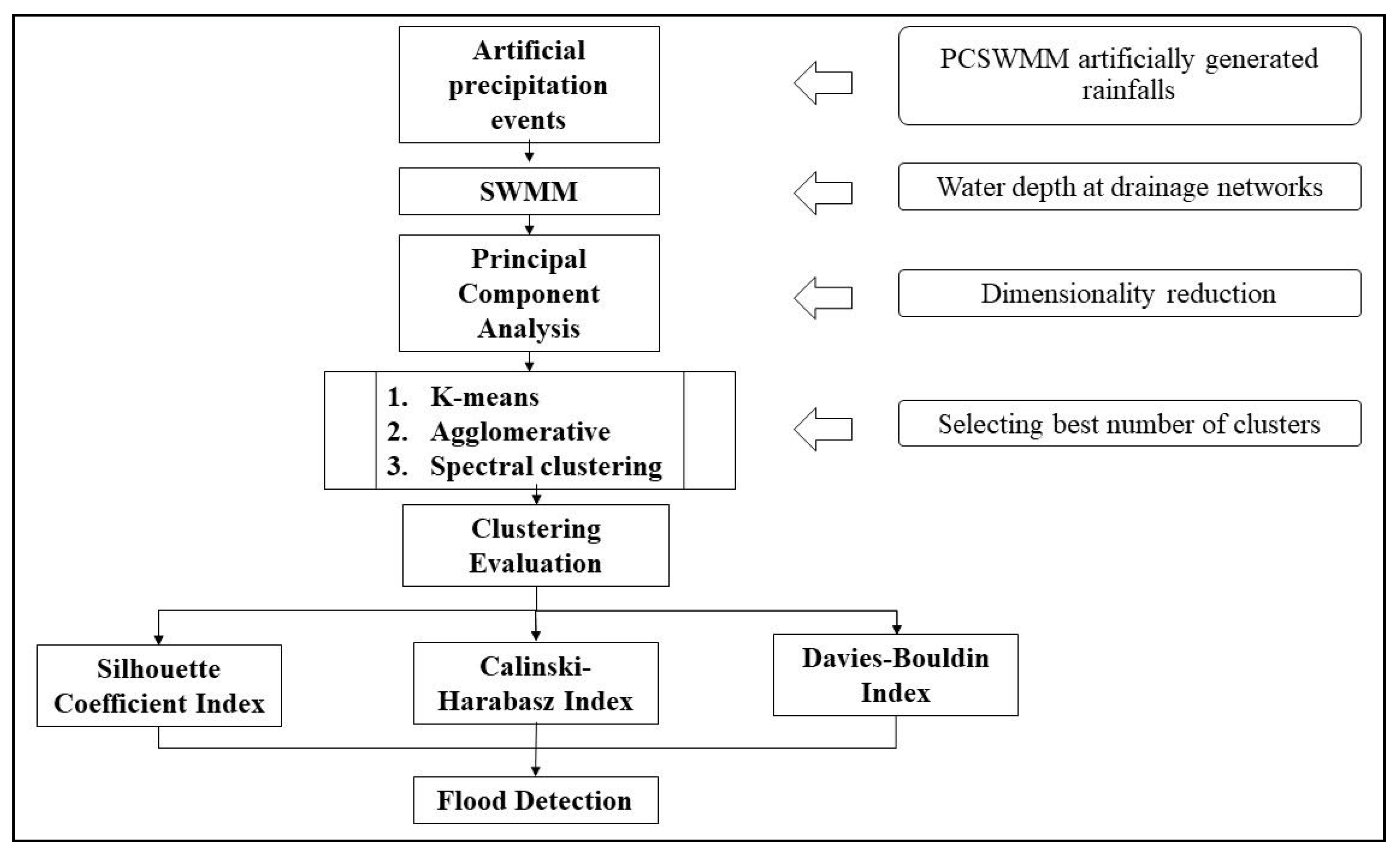
The layout of the study is as follows: (1) build KC, AC, and SC algorithms to group the time-series water depth data; (2) use UMLA metrics, including SCI, CHI, and DBI, to evaluate these algorithms; (3) compare the best number of clusters obtained by each method; (4) investigate the relationship between model performance of flooding detection and water depth data characteristics (see Figure 1 for details). We start by describing the implementation of different UMLA methods, followed by the research methodology with an overview of the real-world case study, performance metrics, and simulation scenarios for cluster analysis. Then, we present the results, discussion, and finally, the conclusions.
2. Materials and Methods
This study was organized in four steps: (i) time-series data preprocessing; (ii) clustering modeling implementation; (iii) clustering performance assessment; (iv) applications analysis of clustering results for urban floods detection. The workflow of the methods can be found in Figure 1.
2.1. Description of Unsupervised Machine Learning Algorithms
Current machine learning techniques mainly fall into two groups: supervised and unsupervised learning [41]. The UMLA is a self-organization method to find patterns in unlabeled data. Cluster analysis is, a subset of UMLA methods, and in general, is based on the principle of grouping similar observations and segmenting dissimilar observations [42]. Anomalous data points that differ from others may then be filtered [43]. A large number of clustering algorithms exist, including K-means, Affinity Propagation, and Mean Shift. In this research, we employed the SCI, CHI, and DBI to assess the performance of the cluster, because of their accuracy and wide applicability in a similar type of studies [44,45,46].
2.1.1. K-Means Clustering
K-means clustering (KC) is a centroid-based unsupervised clustering algorithm, originally designed for signal processing. It is the most widely applied method of cluster analysis in data mining [33]. K-means aims to partition the inputs into k clusters. Given a set of observations (x1, x2, ..., xi) for p variables, the algorithm runs as follows:
- (1)
- Choose k initial centroids, each defined by a value for each of the p variables. These are chosen randomly, often by simply choosing k observations.
- (2)
- Assign each observation to the centroid it is most similar to. The similarity is generally measured as the Euclidean distance between the observation and centroid in parameter space.
- (3)
- Once all observations are assigned, re-estimate the centroids location as the mean of the p variables of all observations assigned to that centroid.
- (4)
- Repeat until the algorithm stabilizes (minimize the within-cluster sum of squares).
The goal then is to minimize the within-cluster sum of squares:
where is the number of cluster centers and {}, = 1, …, k are the cluster centroids . The total intra-cluster distance is the total squared Euclidean distance from each point to the center of its cluster, and this is a measure of the variance or internal coherence of the clusters [47]. This can be used to assess the stability of the solution. When this falls below a predefined threshold, the algorithm stops. The algorithm is often run multiple times with different random initialization of cluster centroids to avoid sub-optimal problems in convergence. The clustering solution with the lowest sum-of-squares is chosen as the final output.
However, the choice of k is challenging when model performance metrics are not available. Often, an initial value of k is chosen, then the algorithm is repeated for higher and lower values. To improve the efficiency of discovering the best k value, a score (SCI, CHI, DBI)-based performance assessment method is recommended in many prior studies [42].
2.1.2. Agglomerative Clustering
Agglomerative clustering (AC) is one of the main forms of hierarchical clustering. These algorithms do not provide a single partitioning of the data but instead provide a full hierarchy of cluster solutions from all observations in a single cluster (i.e., k = 1) to all observations in individual clusters (i.e., k = n) [48]. In contrast to KC, hierarchical methods allow existing clusters to be split or merged, with the result that smaller clusters are related to large clusters in a hierarchy. The rules governing which clusters are again based on their distance or similarity. The AC algorithm consists of the following steps:
- (1)
- Start with each data point as its own cluster.
- (2)
- Select the distance metric and linkage criteria to calculate the dissimilarity between pairs of observations.
- (3)
- Link together the two clusters with the minimum dissimilarity.
- (4)
- Continue this process until there is only one cluster.
A key decision in the AC algorithm is the calculation of dissimilarity between clusters. In this study, we used Euclidean distance [47], and the Ward linkage, which measures the distance between the cluster centroids, similar to the K-means clustering method. The equations for Euclidean distance and Ward linkage are defined by Equations (2) and (3), respectively:
where a and b mean the Euclidean vector; ai and bi are the point position for the Euclidean vector; i is the number of vectors.
where is the squared Euclidean distance between point i and point j; and are Ward’s vectors.
The resulting hierarchy of clusters can be represented using a dendrogram plot [48]. The detailed introduction of the dendrogram plot can be found in Section 2.3.5 below.
2.1.3. Spectral Clustering
Spectral clustering (SC) is an unsupervised learning technique based on graph theory, where SC takes advantage of graph information from the spectrum to find the number of clusters [49]. Unlike the previous methods that tend to prioritize clusters by proximity, SC aims to identify observations that are linked, and therefore may not form classical spherical groups in parameter space. The SC algorithm is as follows:
- (1)
- Create a similarity matrix S between observations. This is the complement to the dissimilarity matrices used in other methods, and here is calculated as the negative Euclidean distance.
- (2)
- Create an adjacency matrix A, representing the graph or connectivity between observations. This is a transformation of S, where for each observation, we find the k nearest neighbors (i.e., with the highest similarity). If observations i and j are considered to be neighbors, we set Aij = Sij. If not, we set Aij = 0.
- (3)
- Create a degree matrix D, where the diagonal values are the degree of connectivity for each observations, given as
- (4)
- Next, calculate the graph Laplacian matrix L. This can be normalized or unnormalized. Here, we use the unnormalized: L = D − A
- (5)
- The clustering solution is then found by eigendecomposition of the Laplacian, and selecting the k smallest eigenvectors. Consequently, these result in a perfect separation of the observations. K-means is then run on these eigenvectors, to get the final cluster assignment of each observation:
As SC performs dimensionality reduction before clustering data points, it is a very flexible approach for complex data sets. However, the similarity matrix generated by SC may include negative values, which can be problematic for grouping time-series points.
2.1.4. Summary and Comparison of Clustering Algorithms
In general, it is difficult to recommend a single algorithm as being the most suitable for clustering, particularly with data that is uncertain and of poor quality, such as the features of pipe flow or water level data used here [41]. It is, therefore, advisable to use several algorithms and compare their performance for specific applications. Here, we use KC, SC, and AC to discover the unknown subgroups in simulated water depth data of UDSs’ junctions. Table 1 summarizes the advantages and disadvantages of these algorithms from review papers [24,33,44].
2.2. Clustering Model Implementation
The SWMM model was run six times, once with each of the rainfall scenarios described above. We collected the simulated time-series water depth from each node in the stormwater drainage network for cluster analysis. As there are 60 junctions in the SWMM model, this results in a matrix where each column represents a single time step with a 5-min interval, and each row (60 rows) stands for a junction or node in the network. We then used the principal component analysis (PCA) to reduce the dimensionality of this matrix. PCA uses the eigendecomposition of the correlation matrix to identify a small set of principal components that represent the majority of variance in the original data [50]. Here, we used correlations between the time-series at different nodes to reduce the column of matrix to 2, which means the number of timesteps is compressed to 2 principal components. Finally, the dataset matrix is configured with 60 rows and 2 columns under each modeling scenarios. The datasets used in this work are not large, and for computational costs are limited. While other techniques for data reduction exist (e.g., correspondence analysis, factor analysis, or non-metric multi-dimensional scaling), we used PCA due to the assumed linear response of the water depth values. Although the reduction of dimensionality might cause data loss or an undesirable relationship between score axes, PCA indeed helps reduce computation time and remove redundant data features in the following cluster analysis.
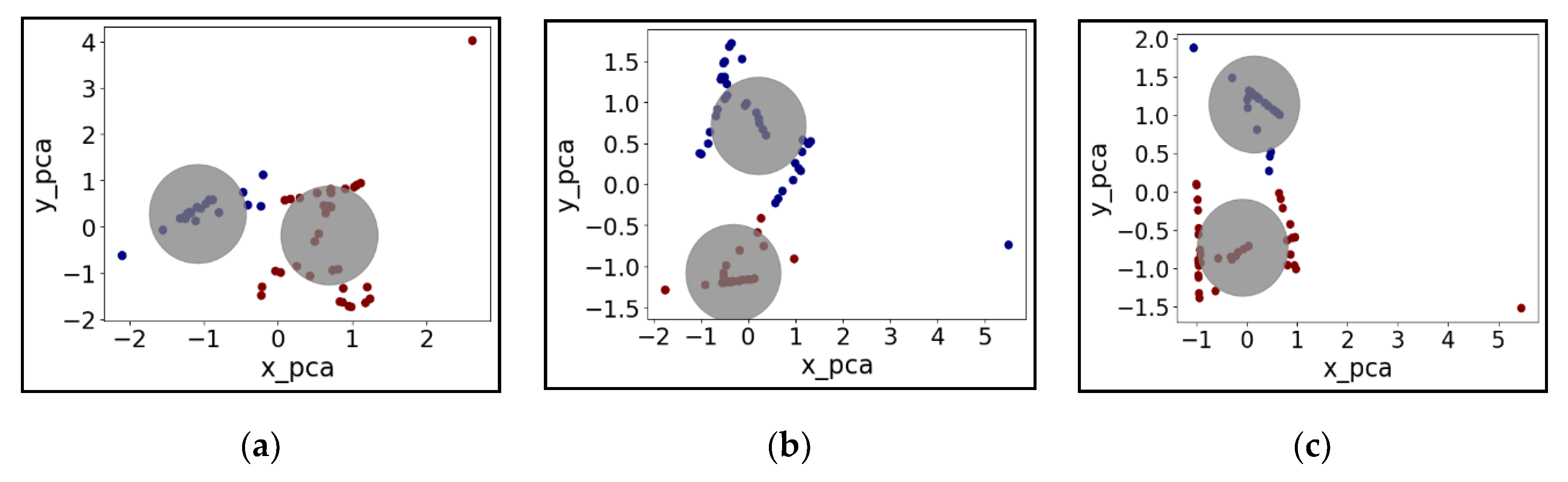
All clustering algorithms were then run using this set of two principal components shown in Figure 2, with the following set up:
- (1)
- K-means: We initially set the number of clusters (k) to 2 for each modeling scenarios. The algorithm was repeated ten times with different random initialization, and a maximum of 5 iterations was used to converge the algorithm.
- (2)
- Agglomerative clustering model: We used Ward linkage, as this is robust to outliers and unequal variance in the data. As only ‘Euclidean’ supports ‘Ward’ linkage distance computation. If ‘Ward’ linkage is used for cluster distance computation, ‘Euclidean’ would be the best way to measure the data dissimilarity [51]. Thus, the cluster distance calculation method and dissimilarity metric among sample points are set to be ‘Ward’ and ‘Euclidean’ distance, respectively. The resulting hierarchy was cut to provide 2 clusters.
- (3)
- Spectral clustering: The algorithm was used to identify 2 clusters, using the unnormalized graph Laplacian.
In Figure 2 below, there is no sample marginal overlapping, which indicates the cluster classification is reasonable with respect to grouping the time-series water level data. Additionally, the isolated dots in the subplots of Figure 2 present the dissimilarity of the water depth datasets under this event, indicating these isolated dots might be the potential flooded junctions, which help the decision-makers to pre-screen the vulnerable sites in the drainage networks.
2.3. Clustering Model Evaluation and Validation
Unlike the supervised machine learning algorithms that compare the predicted and actual values to compute the model accuracy, the UMLA assess performance directly on the characteristics of the clusters that were obtained. The performance then depends on data features selected, data preprocessing, and parameter settings such as the distance function to use, a density threshold, or the number of expected clusters, which can be modified according to the varying datasets and object inputs. As a result, there is rarely a single obvious solution for clusters, and cluster analysis is an iterative process of knowledge discovery or interactive multi-objective optimization that involves trial and failure, aimed to obtain the desired results [52,53,54,55].
Several indices, including SCI, DBI and CHI, are employed to measure the relative performance of clustering algorithms. In general, these metrics provide an assessment of how the data variance is partitioned. An ideal cluster solution will have low intra-cluster variance (i.e., all observations should be similar within a cluster) and high inter-cluster variance (the clusters should be well separated).
2.3.1. Silhouette Coefficient Index
The silhouette coefficient index is an example of model-self-evaluation, where a higher SCI score relates to a model with better-defined clusters [56]. This score is bounded between −1 for incorrect clustering and +1 for well-formed clusters. Scores around zero indicate overlapping clusters. The SCI is defined for each observation, which can be calculated as Equation (4):
where the is for a single observation; m is the mean distance between an observation and all other observations in the same class; is the mean distance between the same observation and all observations in the next nearest cluster. The SCI has the advantage that it can be used to examine how well individual observation are clustered, or an estimate can be obtained for each cluster or for the whole cluster solution by averaging across a cluster or the entire dataset, respectively. An estimate can be obtained for each cluster or for the whole clusters solution. A set of samples is given as the mean of the SCI for each sample, and it would be relatively higher when clusters are dense and well separated [57].
2.3.2. Calinski-Harabasz Index
The CHI is calculated as the ratio of the between-clusters dispersion average and the within-cluster dispersion [58], penalized by the number of clusters (k). A higher CHI score indicates better-defined clusters (i.e., dense and well separated). CHI for a set of k clusters is calculated as:
where is the number of points in our data; is the number of the cluster; represents dispersion matrix; is the between-group dispersion matrix, and is the within-cluster dispersion matrix. and are defined by the following equations:
where is the set of points in the cluster , is the center of the cluster , is the center of the whole data set which has been clustered into k clusters, is the number of points in the cluster .
2.3.3. Davies-Bouldin Index
The DBI can also be used to evaluate the model, where a lower DBI relates to a model with better separation between the clusters [59]. The index is defined as the average similarity (Rij) between each cluster k and the next closest (i.e., most similar) cluster. The DBI is calculated as Equation (8):
where is the Davies–Bouldin index. Zero is the lowest possible score. Values closer to zero indicate a better partition. is the number of the cluster. is the similarity measure which features per Equation (9):
where is the average intra-distance between each point of cluster i and the centroid of that cluster representing as cluster diameter; is the inter-cluster distance between cluster centroids i and j; is set to the trade-off between inter-cluster distance and intra-cluster distance. The computation of DBI is simpler than that of SC since this index is computed only with quantities and features inherent to the dataset [60]. However, a good value reported by DBI might not imply the best information retrieval [55].
2.3.4. Intra-Cluster Distance
Intra-cluster distance (ICD) is the distance between two samples belonging to the same cluster. Three types of intra-cluster distance, including complete diameter distance, average diameter distance, and centroid diameter distance, are popular in prior studies. As the number of clusters increase, individual clusters become more homogenous, and the ICD decreases. At a certain point, the decrease in distances becomes negligible. Plotting this distance against k usually results in an inflection point or elbow point where this occurs, and can be used to identify the optimal value of k [61]. The number of clusters is chosen at this point, hence the "elbow criterion." Here we use the centroid distance to represent ICD, given as double the average distance between all of the objects:
where is the centroid diameter distance of the formed cluster representative ; is the samples belonging to cluster is the distance between two objects, x and ; |S| is the number of objects in cluster .
2.3.5. Dendrogram
A dendrogram is a visualization in the form of a tree that shows the hierarchical relationship like the order and distance (dissimilarity) between samples [62]. The individual samples are located along the bottom of the dendrogram and referred to leaf nodes. The hierarchical clusters are formed by merging individual samples or existing lower-level clusters. In a dendrogram, the vertical axis is labeled distance and refers to a dissimilarity measure between individual samples or clusters. Generally, in a dendrogram, horizontal lines can be regarded as places where clusters merge, while vertical lines show the distance at which lower-level clusters were merged, forming a new higher-level cluster. The dissimilarity measure between two groups is calculated as Equation (12):
where Dis means the dissimilarity or distance among objects and C means the correlation degree between clusters.
If clusters are highly correlated to each other, they will have a correlation value close to 1. To that, Dis = 1 − C will be given a value close to zero. Therefore, highly related clusters are nearer to the bottom of the dendrogram. Those clusters that are not correlated have a correlation value close to zero. Clusters that are negatively correlated will give a distance value larger than 1 in the dendrogram. The dendrogram can be used to visually allocate correlated objects to clusters or to detect outliers and anomaly in a diagram [47]. In the dendrogram, each sample is treated as a single cluster and then successively combines pairs of clusters until all clusters have been merged into a single cluster. In this process, the dendrogram shows how the aggregations are performed from bottom to top of the dendrogram statically. This procedure allows the cut-off points to flexibly and efficiently represent the number of clusters. Therefore, this study used the number of cut-off points in the dendrogram to validate the cluster number of the agglomerative clustering.
2.4. Study Area and Data Description
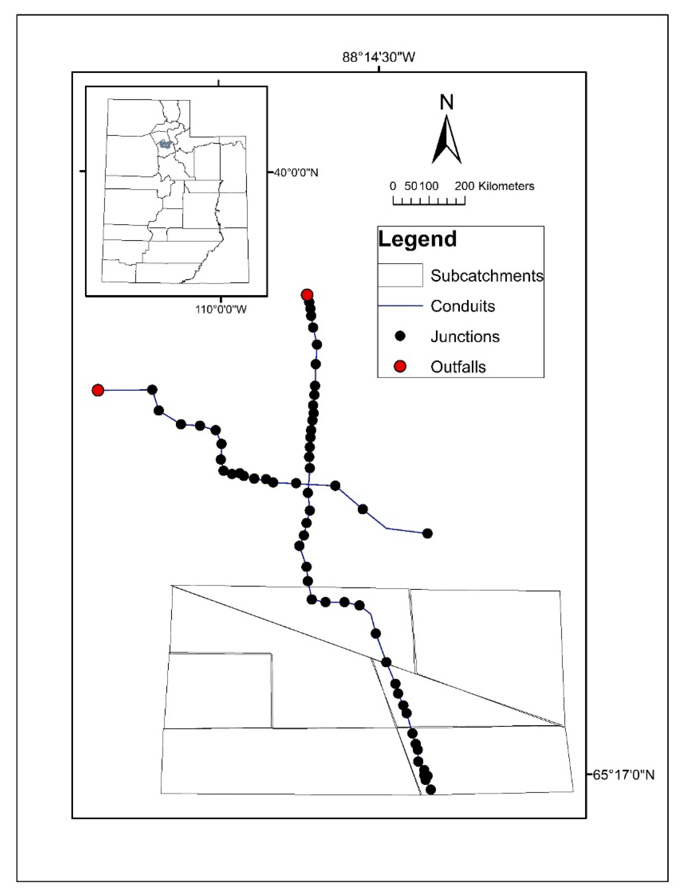
A real-world urban stormwater system located in Salt Lake City, UT, U.S., was selected as the case study, shown in Figure 3. This study case, with an area of 81-ha, is semi-arid, and has soil composed of four primary types: alluvial fan, artificial fill, silt and clay, and sand and gravel deposits. The soil surrounding the study area is classified as hydrologic soil groups B and C, with low infiltration capacity, which has a relatively poorly draining surface. Due to climate change and urbanization, the studied area has suffered from floods more frequently than 1990s, and the increase in the magnitude and duration of the storm events has pushed the resulting stormwater system out of service. This urban drainage network was represented by a rainfall-runoff SWMM model. SWMM is a state-of-art tool developed to help support local, state, and national stormwater management objectives to reduce runoff, discharge, and improve stormwater quality [63,64]. It has been widely used all over the world in similar type of investigations including stormwater runoff, combined and sanitary sewers, and other drainage systems [65,66,67]. Figure 3 shows the components of this SWMM model, which includes one rain gauge, 60 junctions, 61 conduits, two outfalls, and seven sub-catchments, while the groundwater interflow, water evaporation, snowmelt, and manhole hydraulic loss are neglected during the simulation [68].
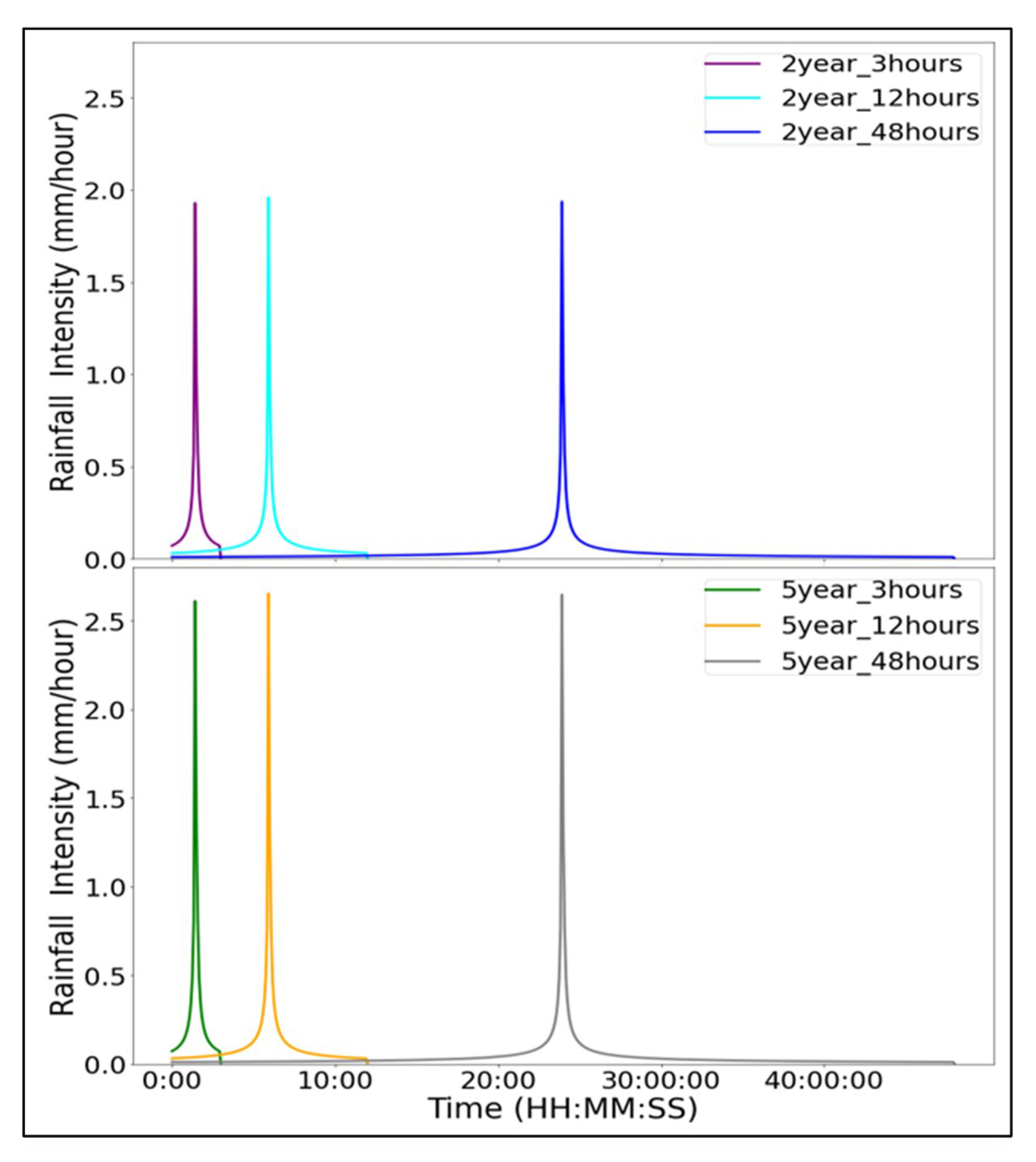
For this study, we created 6 artificial precipitation series according to the Chicago distribution method in PCSWMM v.7.3, and then imported them as modeling inputs. The distribution for the synthetic rains is shown in Figure 4. These rainfalls with durations of 3 h, 12 h, to 48 h and return periods ranging from 2-year to 5-year almost contain all typical features and characteristics of real storms in the study area. Additionally, rainfall measurements for two real rainfall events were collected to test the clustering algorithm. These rain records from 5 May 2015 rainfall event and 8 July 2015 rainfall event are representative for the typical real storms under average climatic conditions in the study area. Compared with water depth generated by the artificially designed rainfall data, the time-series water depth produced by the real-world storms contains more non-stationarity and noise. Nevertheless, the obtained findings are subsequent validated with real rain records.
3. Results
3.1. Clustering Performance Evaluation
3.1.1. K-Means
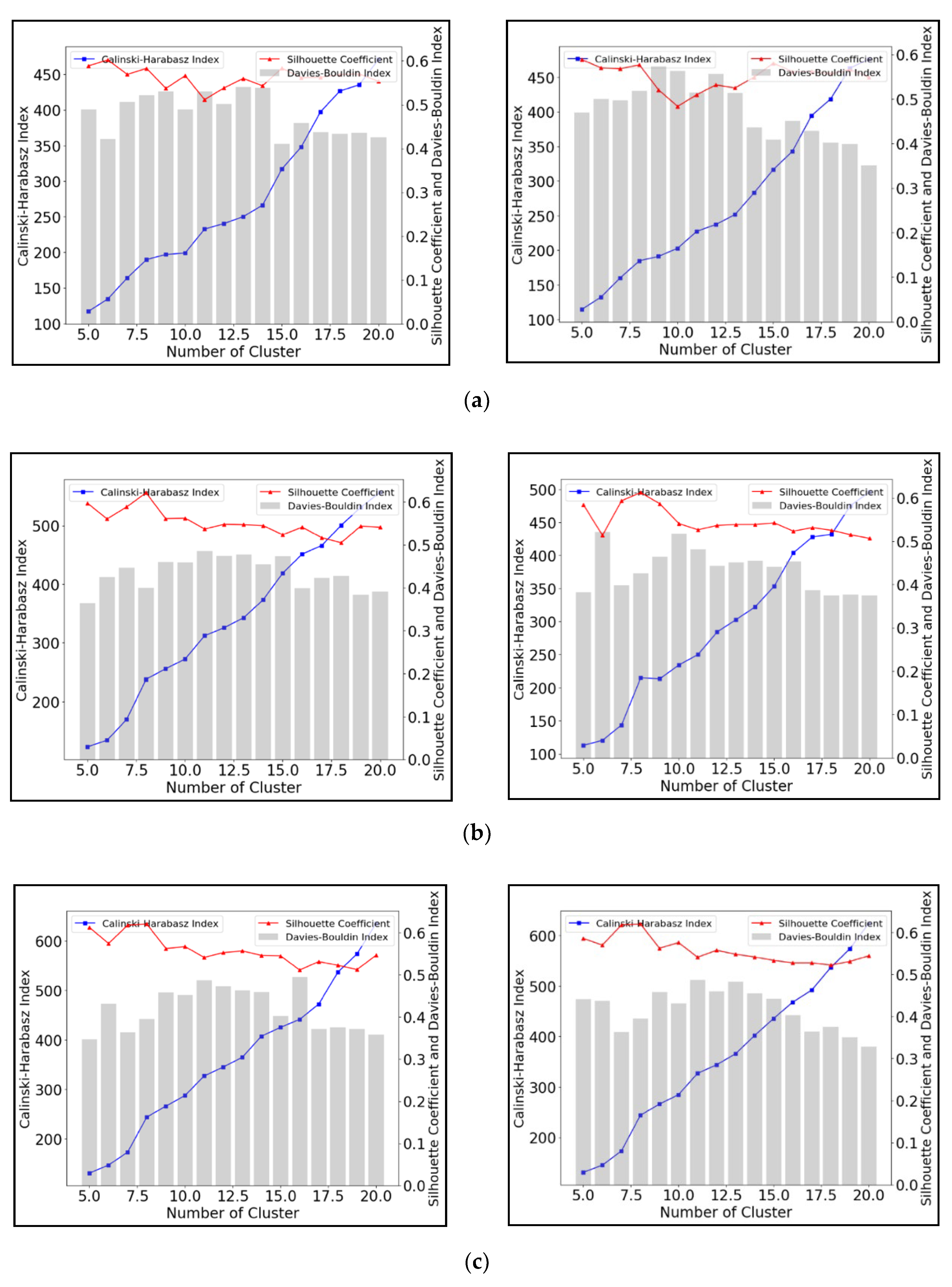
A detailed investigation was carried out to assess the performance of the clustering algorithms. Figure 4 shows how three performance metrics SCI, CHI and DBI change with different cluster numbers when using K-means to cluster the time-series water depth data. Values for the CHI value increase with higher cluster numbers, whereas the SCI and DBI values fluctuate. The SCI and DBI values show opposite trends, reflecting the different methods by which they are calculated (see Section 2.3 above). In particular, Figure 5b,c show that the best solution is with eight clusters, reflected in the largest SCI value and smallest DBI value. These results suggest that the SCI and DBI are more suitable to assess the performance of K-means, while any peak in the CHI related to cluster quality is eclipsed by the influence of increasing the number of clusters. Based on the SCI and DBI value in Figure 5a, the optimal number of clusters is six for the two year-3 h and five year-3 h rainfall scenarios. The differences in the optimal number of clusters in Figure 5a–c indicate that rainfall duration has impacts on the number of clusters when utilizing K-means to group time-series water depth datasets.
3.1.2. Agglomerative Clustering
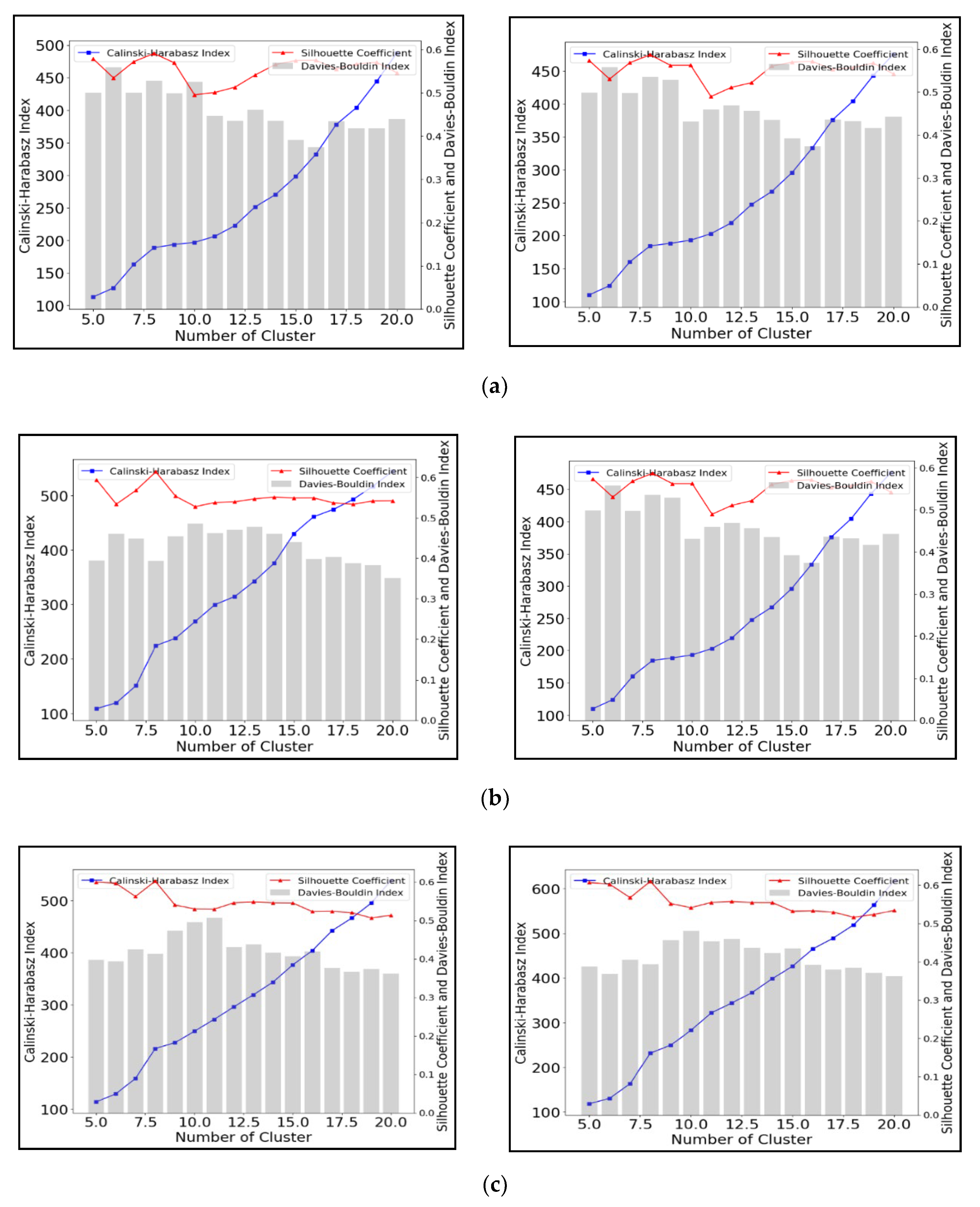
Figure 6 shows the same results but based on the use of Agglomerative Clustering (AC) to group the time-series water depth data. As with the K-means results (Figure 5), the CHI value increase with the number of clusters for all scenarios from short-duration to long-duration rainfall. Again, it is difficult to identify an optimal number of clusters, and this suggests that the CHI is not suitable for ascertaining the best clustering solution with these data. In contrast, the SCI and DBI show clear peaks in their values. Figure 6a shows that 16 clusters result in the maximum SCI close to 0.76 and minimum DBI with 0.38. Figure 5c shows a peak in SCI values (~0.6) for eight clusters, with a corresponding minimum in the DBI value (<0.4). However, Figure 6b shows that eight clusters could produce the largest SCI (~0.62) and the lowest DBI (~0.40) with the two year-12 h rainfall duration scenario (left subplot), but that 16 clusters are the optimal solution for the two year-12 h rainfall (SCI ~0.58 and DBI ~0.38; right subplot). In summary, the best cluster solutions AC algorithms are 16, eight, and eighteen under 3 h, 12 h, and 48-h duration rainfalls, respectively. Comparing the left subplots with the right subplots (Figure 6) provides evidence that the cluster number for the best AC performance remains the same, although the return period has been shifted from two-year to five-year. The rainfall return period (annual exceedance probability) was found to be less related to the number of clusters.
3.1.3. Spectral Clustering
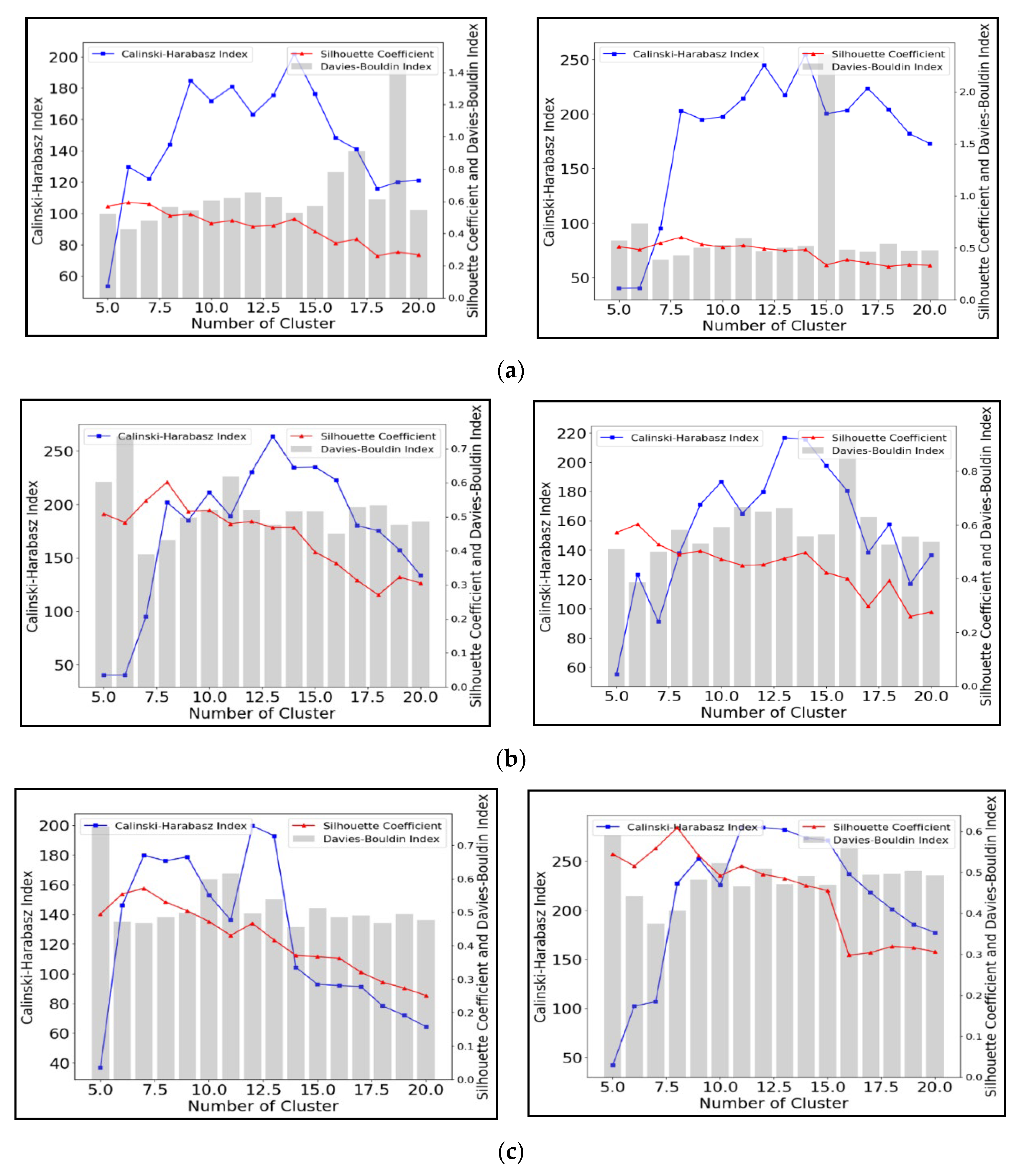
Figure 7 shows the results obtained for different cluster numbers using Spectral Clustering to group the time-series water depth data. In contrast to the two previous methods, the SCI values decrease as the number of clusters increase. For the 12 and 48 h scenarios, this index identifies solutions at about 6–7 clusters, but no clear optimal solution is identified in the shorter scenarios (panel a). This suggests that this index is unsuitable for assessing this algorithm. The DBI values show greater variation as the number of clusters change, although minima can be observed at 6 to 7 clusters for most scenarios. The CHI values no longer show a linear increase, but show clear peaks, although usually for higher numbers of clusters than the DBI identifies. The highest CHI values (275 for 2 year-12 h and 190 for 5 year-12 h) are all generated by the SC with 13 clusters. For the for two year-48 h and five year-48 h scenarios, the largest CHI values are approximately 200 and 270, respectively, in both cases for 12 clusters.
3.2. Clustering Performance Testing
The analysis of cluster performance in the previous section is based on synthetic rainfall datasets, due to lack of water depth data in the drainage network. However, the use of noise-free synthetic data may have a significant impact on the results obtained [69], and our results may not represent real storm situations or current climate conditions. In contrast, the trends identified here might be masked by time series noise, making it more difficult to identify optimal solutions. In order to validate that the results obtained from designed rainfalls can also be applied to non-stationary real-storms, we evaluate the performance of the clusters in grouping flooding water depth datasets generated by two real flood events described below.
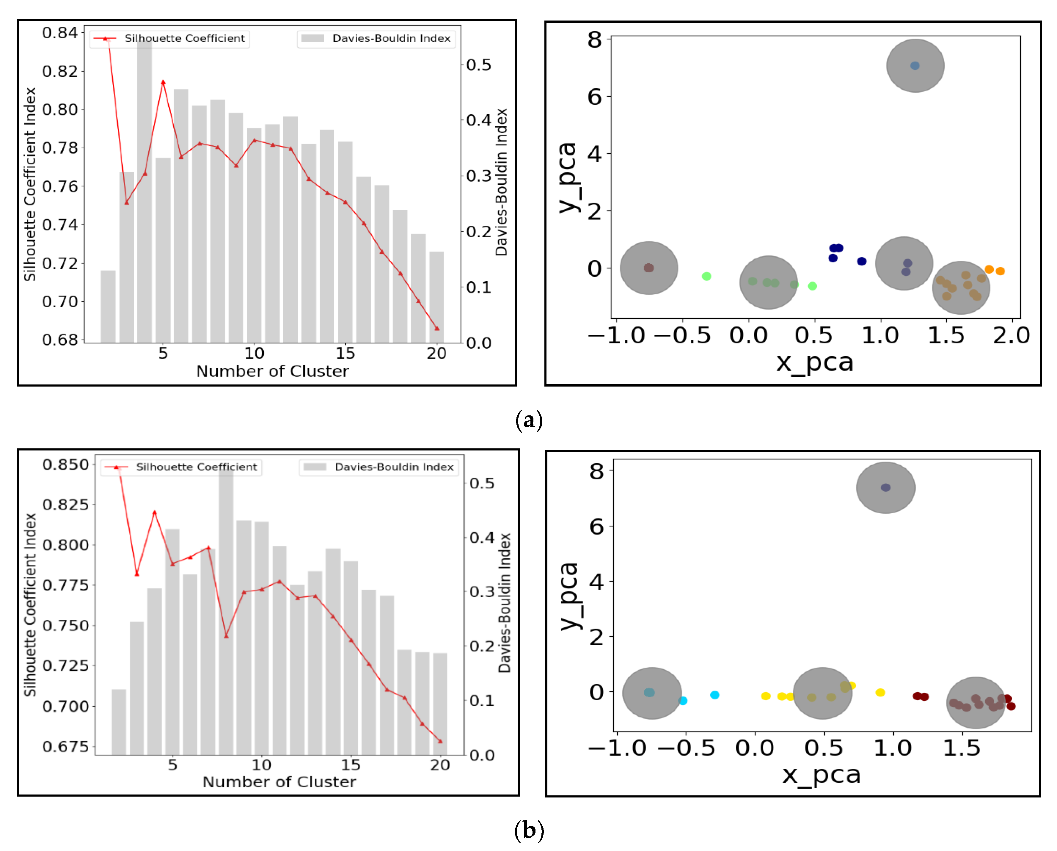
The left plot in Figure 8 indicates that the best number of clusters for the 5 May 2015 event (Figure 8a) and 8 July 2015 event (Figure 8b) are five and four, respectively. Increasing the number of clusters beyond this causes both the SCI and the DBI to decline. The distribution of different clusters obtained is shown in the PCA plots in the right panel of Figure 7. These show that the cluster analysis resulted in a good separation of the storm events (indicated by the lack of overlap between the gray circles).It should be noted that both subplots 8a and 8b have an isolated cluster on the top. This is the only cluster composed of one sample, which means the water depth from the corresponding junction is significantly distinguishable to others. One possible reason for this phenomena is that the flooding or overflow events have occurred, triggering a very different signal in water depth at this location. Besides, as the rainfall duration increases from 3 h (the 5 May 2015 storm) to 24 h (the 8 July 2015 storm), the reduction in the number of clusters selected is in line with the results of Section 4, supporting the negative correlation between the number of clusters and event duration.
3.3. Cluster Number Validation
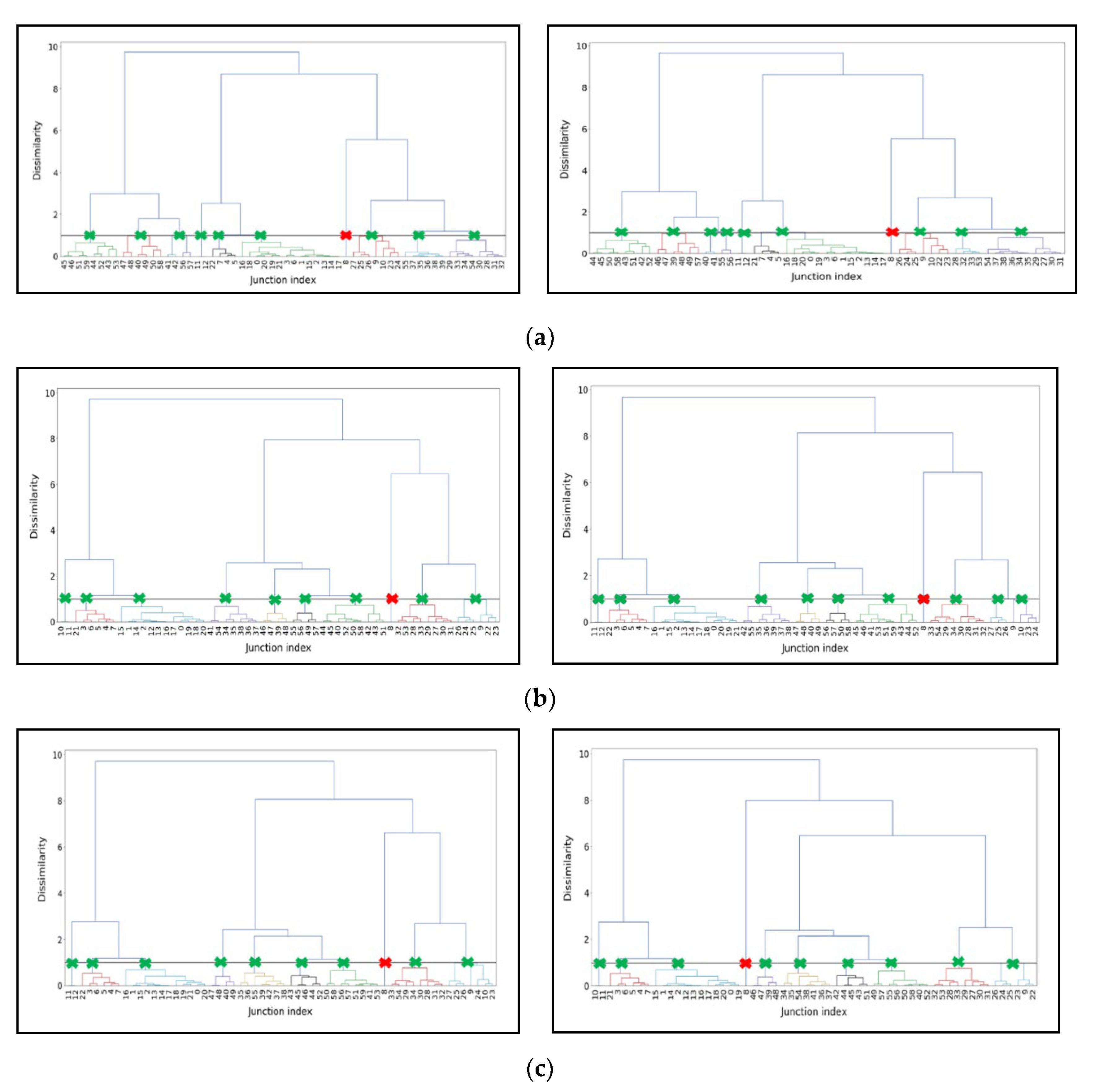
The dendrogram plots are also used to validate the number of clusters. Figure 9 shows the dendrogram plots obtained from applying the AC algorithm to the flooding water depth data. Generally, the cut-off point should be at least 70% dissimilarity between two clusters or cutting where the dendrogram difference is most significant [69]. The number of clusters was selected by using a distance threshold of 0.9 distance or 90% dissimilarity, and this is plotted as a horizontal cut-off line in all dendrograms of Figure 9. The cross points (highlighted as green X in dendrogram) between the cut-off line and dendrogram leaves identify the accepted clusters. In Figure 9, one point identified by the cut-off line (junction 8; highlighted as red X in dendrogram) was considered as an outlier in the dendrogram and excluded. In practice, this algorithm might be helpful for anomaly detection in the sensor monitoring network. For instance, real-time monitoring is built to capture the varying different features of measurements as much as possible within a limited number of sensors [70,71]. Further, the clusters represent different parts of the hydrological network and can be used to help target locations for sensor deployment to observe overflow and flood events in the field.
The vertical comparisons among the subplots of Figure 9a–c disclosed that the appropriate cluster numbers for 3 h, 12 h and 48 h rainfall scenarios are quite similar: eight, nine, and nine, respectively. Meanwhile, comparing cluster solutions for different time periods (e.g., left and right plot of Figure 9a, the number of clusters and their structure is remarkably similar, implying that the event return period has fewer impacts on AC model performance. This supports the conclusions reached with the synthetic time series, that the AC model performance noticeably depends on the flooding duration but not the event return period (exceedance probability).
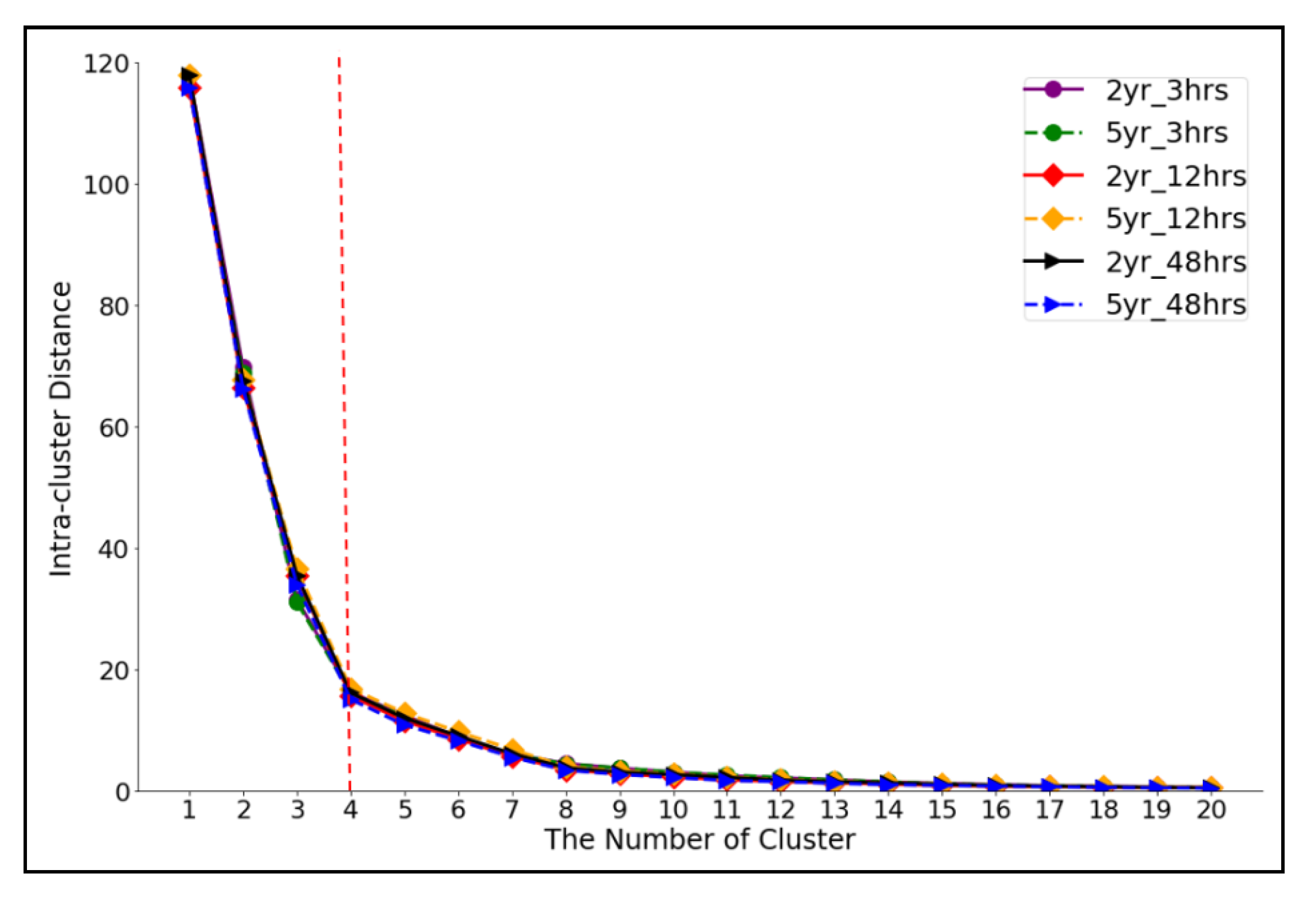
This study adopted intra-cluster distance as the metric to assess the effects of flooding duration and return period (exceedance probability) on the performance of the K-means and Spectral Clustering algorithm. Figure 10 shows the results of this comparison, with the decay in the intra-cluster distance as the number of clusters increases. A notable elbow point (the cross between red dashed line and intra-distance curves) can be seen at the four clusters, as the decrease in distances becomes much smaller. Using the elbow criterion described in Section 2.3.4, this suggests that four clusters are the best solution. Increasing the number of clusters beyond this would result in a little additional gain for the extra complexity of the solution. Figure 10 shows that the intra-cluster distance changes in a similar way for all six rainfall scenarios, and that the intra-cluster distance is close in those rainfalls with the same duration. For example, the solid purple line with purple circle markers (representing two year-3 h rainfall scenario) overlaps the red dashed line with the red circle markers (representing five year-3 h rainfall scenario). However, there are still some differences between scenarios with different rainfall duration. Notably, the intra-cluster distance increases as the rainfall duration decreases (the distance for the ‘3 h’ duration rainfall is the largest, followed by the ‘12 h’ cases, and then the ‘48 h’ scenarios). As a metric for clustering performance, intra-cluster distance is therefore useful in determining how well these algorithms group the water depth time-series. These results suggest that the K-means and spectral clustering algorithms work best with longer duration rainfalls, implying that the longer event duration produces greater similarity in the water depth at different junctions. This, coupled with the larger set of observations from a longer period, results in better formed individual clusters. Wu et al. have shown that these cluster methods work optimally when trained on massive datasets, which is supported by the results herein [72].
4. Discussions
4.1. Clustering Parametric Discussion
Previous cluster-based studies have mainly focused on detecting pressure, demand, pipe burst, infrastructure damage, and illicit intrusion in water distribution systems [71,72,73]. In the cluster analysis here, the features, such as the length of time-series water depth from UDSs, are found to be negatively correlated with the number of clusters. This finding has been validated by the dendrogram cut-off points in those designed rainfalls and also by the cluster center mapping based on real storm events. The similar results between the artificial (noise-free) and practical (noise-polluted) scenario infer that event duration (data length) overwhelms the event exceedance probability (data magnitude) in the cluster number identification, which agrees with the findings from [25,72]. Increasing the number of clusters often results in many more errors. One extreme case is that the zero error happens when each data point is equal to every cluster. Intuitively, the choice of the best number of clusters can be interpreted into a trade-off between the maximum reduction of complexity of the data with a single cluster and maximum accuracy by assigning each data point to its cluster. For long time series, we suggest starting with a small number of clusters and increasing the number, testing the performance at each increase.
In addition to the determination of the number of clusters, the structure of datasets may also affect the clustering model performance. KC and SC algorithms are able to robustly group water depth datasets from longer duration flood events. However, there is a limited relationship between algorithm performance and annual exceedance probability. The sharply rising trend (Figure 4, Figure 5 and Figure 6) demonstrates that the CHI is not suitable to identify the best number of clusters in the KC and AC algorithms, but that the SCI and DBI work quite well and give comparable results (Figure 4, Figure 5 and Figure 6). In contrast, the CHI works well in identifying the optimal cluster number with the SC algorithm. This difference reflects the different nature of the algorithms: KC and AC are based on simple dissimilarity measures between observations, whereas the SC is based on a graph representing connectivity. This is because that DBI evaluates intra-cluster similarity among every data point and inter-cluster differences among each group. Similarly, the SCI measures the distance between each data point and the centroid of the cluster it was assigned to. An SCI value close to 1 is always good, and a DBI value close to 0 is also good whatever clustering you are trying to evaluate. However, the CHI is not normalized, and it is difficult to compare two values of the CHI index from different data sets.
4.2. Implications of Clustering Application
This study provides an understanding of different clustering algorithms, applicability with different datasets, and an assessment of cluster solutions in flood detection strategies. For instance, as water level is one of the inferential indicators of local flood events, clusters with abnormal water level can be identified as early warning signals of flooding. As new data become availabel during monitoring, these can be assigned to the most similar cluster. Decreasing dissimilarity to abnormal cluster therefore indicates increasing likelihood of flooding. In Figure 8, we observed that there is one isolated dot for each subplot. These separated points represent the highly dissimilar water depth data, indicating the possibility of triggering flood events. These same cases are also captured in the dendrogram of Figure 9 which presents that the junction 8 highlighted with red cross might be the source of anomalous water level. One reasonable explanation for the anomalous cluster is the resultant flooding or overflow events occuring around the corresponding location. More attention are recommended to investigate if this location is flooded. Thus, it can be seen that classifying these points as anomalies is helpful for narrowing down the spatial searching domain from network-level to node-level, and consequently also reducing the timing and efforts in identifying the flooded locations in the complex network system [74,75,76]. We concluded that the occurrence of anomalous changes in water level in UDSs could be a timely reminder of the upstream or downstream overflow events for the neighborhoods. Our findings also explain how the characteristics of the dataset (notably length and magnitude) influence the number of clusters. This information could be employed to detect urban flood events using water depth datasets in other real drainage networks [66,67]. These clustering algorithms aim to efficiently capture the urban drainage flooding locations providing a basis for managing the existing drainage structures and developing sustainable urban drainage networks in urbanized areas [77].
4.3. Limitations and Future Work
Although this study has identified some clear differences in the application of cluster analysis, there are several limitations. Firstly, the majority of scenarios used time-series water depth datasets generated by model simulation. As these are smooth and noise-free, the results may not scale to field application. However, we found similarities between the results with the limited set of observed rainfall series used here, notably in the use of the different indices, but tend to result in a smaller number of clusters. Further work should apply these methods to a wider set of observed data to reduce the input (meteorological) uncertainties and meteorological variances if such data becomes available [36,37,78,79]. The possible integration of ensemble prediction system (EPS) and data assimilation techniques might be of interest for future work, which could provide help for estimating forecast uncertainty via a linear combination of suitable meteorological variances and uncertainties linked to the rainfall and hydraulics [80,81]. Secondly, as this paper only focuses on exploring usefulness of clustering model implementation and performance evaluation, analysis of errors and sensitivity analysis of water level datasets are recommended for to improve the reliability of results. Future work will concentrate on the application of these methods, including water-level sensor placement, combined sewer overflow detection, and urban flooding prediction. Since the dendrogram enables the AC algorithm to detect outliers in time-series water depth datasets, this can be used to help guide sensor deployment on vulnerable sites for observing overflow and flood events in the field [76]. It is planned to consider strengthening the connection between the theoretical results and field application by conducting a cluster analysis to optimize the sensor monitoring network for flooding detection at UDSs.
5. Summary and Conclusions
In the age of ‘smart stormwater,’ the increased deployment of sensors to monitor water level characteristics is resulting in rapidly accumulating data. It is becoming crucial to understand and promote methods to handle these big datasets to help in flood detection and control. This study aims to promote understanding of how cluster analysis facilitates the interpretation of the unlabeled time-series water depth data for flooding location detection at the stormwater urban drainage systems. In this work, three indexes, including silhouette coefficient index, Calinski–Harabasz index, and Davies–Bouldin index, were used to evaluate the performance of three popular unsupervised cluster analysis models namely K-means clustering, agglomerative clustering and spectral clustering. A real-world stormwater urban drainage systems SWMM model was applied to test the performance of clustering algorithms in capturing urban floods. Five conclusions were drawn below:
- (1)
- Silhouette coefficient index and Davies–Bouldin index are suitable metrics to measure the performance of K-means and agglomerative clustering model when subject to identify the number of clusters for the best performance. However, the Calinski–Harabasz Index is found to be more favorable to assess the performance of the spectral clustering model in grouping time-series water depth datasets for urban drainage flooding detection.
- (2)
- In K-means and spectral clustering models, the number of the clusters for maximizing model performance is highly related to the dataset length (flooding duration) but is slightly associated with the dataset magnitude. There is a negative correlation between the number of clusters and the length of datasets.
- (3)
- The short-period water depth data can be well-grouped by the agglomerative clustering model. In contrast, K-means and spectral clustering models are better able to handle time-series water depth datasets from long-duration storm scenarios.
- (4)
- This research work provides insight into unlabeled hydraulic data-driven techniques by conducting clustering experiments. The outcomes are useful for researchers to select the appropriate clustering model and to choose the corresponding performance metrics for specific urban flooding applications.
- (5)
- The detailed analyses in this work provide guidance concerning how to use cluster solutions to isolate or prescreen vulnerable locations for flooded location detection strategies. The water level in isolated clusters can be considered as the floods early warning for the local residents. The occurrence of anomalous changes in water level in urban drainage systems could be a timely reminder of the upstream or downstream flood events for the surrounding neighborhoods.
Author Contributions
Conceptualization, J.L.; Data curation, J.L.; Formal analysis, J.L. and D.H.; Funding acquisition, J.L. and R.S.; Investigation, J.L., D.H., and S.B.; Methodology, J.L. and S.B.; Resources, R.S.; Software, J.L.; Validation, J.L.; Visualization, J.L. and D.H.; Writing—original draft, J.L.; Writing—review & editing, D.H., S.B., and R.S. All authors have read and agreed to the published version of the manuscript.
Funding
This research is funded by the Research Assistant Scholarship at the University of Utah. The contribution of the University Innsbruck is financially supported by the Austrian Climate and Energy Fund and by the programme "Smart Cities Demo - Living Urban Innovation 2018" (project 872123).
Acknowledgments
We would like to thank the Salt Lake City Department of Public Utilities (SLCDPU) for their efforts in developing the SWMM model. We also thank the Computational Hydraulics Int. (CHI) company for offering the research license of PCSWMM. Finally, we thank Steven Burian and the Student Engineering Association (SAE) of the University of Utah for sharing their relevant files and materials.
Conflicts of Interest
The authors declare no conflict of interest.
References
- Li, J.; Tao, T.; Kreidler, M.; Burian, S.; Yan, H. Construction Cost-Based Effectiveness Analysis of Green and Grey Infrastructure in Controlling Flood Inundation: A Case Study. J. Water Manag. Model. 2019, 27, C466. [Google Scholar] [CrossRef] [Green Version]
- Kerkez, B.; Gruden, C.; Lewis, M.; Montestruque, L.; Quigley, M.; Wong, B.; Bedig, A.; Kertesz, R.; Braun, T.; Cadwalader, O.; et al. Smarter stormwater systems. Environ. Sci. Technol. 2016, 50, 7267–7273. [Google Scholar] [CrossRef]
- Li, J.; Yang, X.; Sitzenfrei, R. Rethinking the framework of smart water system: A review. Water (Switzerland) 2020, 12, 412. [Google Scholar] [CrossRef] [Green Version]
- Morales, V.M.; Mier, J.M.; Garcia, M.H. Innovative modeling framework for combined sewer overflows prediction. Urban Water J. 2017, 14, 97–111. [Google Scholar] [CrossRef]
- Norbiato, D.; Borga, M.; Degli Esposti, S.; Gaume, E.; Anquetin, S. Flash flood warning based on rainfall thresholds and soil moisture conditions: An assessment for gauged and ungauged basins. J. Hydrol. 2008, 362, 274–290. [Google Scholar] [CrossRef]
- Wong, B.P.; Kerkez, B. Adaptivemeasurements of urban runoff quality. Water Resour. Res. 2016, 52, 8986–9000. [Google Scholar] [CrossRef]
- Solomatine, D.P.; Ostfeld, A. Data-driven modelling: Some past experiences and new approaches. J. Hydroinformatics 2008, 10, 3–22. [Google Scholar] [CrossRef] [Green Version]
- Henonin, J.; Russo, B.; Mark, O.; Gourbesville, P. Real-time urban flood forecasting and modelling—A state of the art. J. Hydroinformatics 2013, 15, 717–736. [Google Scholar] [CrossRef]
- Koo, D.; Piratla, K.; Matthews, C.J. Towards Sustainable Water Supply: Schematic Development of Big Data Collection Using Internet of Things (IoT). Procedia Eng. 2015, 118, 489–497. [Google Scholar] [CrossRef] [Green Version]
- Vojinovic, Z.; Abbott, M.B. Twenty-five years of hydroinformatics. Water 2017, 9, 59. [Google Scholar] [CrossRef] [Green Version]
- Diao, K.; Farmani, R.; Fu, G.; Astaraie-Imani, M.; Ward, S.; Butler, D. Cluster analysis of water distribution systems: Identifying critical components and community impacts. Water Sci. Technol. 2014, 70, 1764–1773. [Google Scholar] [CrossRef] [PubMed]
- Kang, O.Y.; Lee, S.C.; Wasewar, K.; Kim, M.J.; Liu, H.; Oh, T.S.; Janghorban, E.; Yoo, C.K. Determination of key sensor locations for non-point pollutant sources management in sewer network. Korean J. Chem. Eng. 2013, 30, 20–26. [Google Scholar] [CrossRef]
- Mullapudi, A.; Lewis, M.J.; Gruden, C.L.; Kerkez, B. Deep reinforcement learning for the real time control of stormwater systems. Adv. Water Resour. 2020, 140, 103600. [Google Scholar] [CrossRef]
- Tehrany, M.S.; Pradhan, B.; Jebur, M.N. Flood susceptibility mapping using a novel ensemble weights-of-evidence and support vector machine models in GIS. J. Hydrol. 2014. [Google Scholar] [CrossRef]
- Yu, P.S.; Yang, T.C.; Chen, S.Y.; Kuo, C.M.; Tseng, H.W. Comparison of random forests and support vector machine for real-time radar-derived rainfall forecasting. J. Hydrol. 2017, 118, 489–497. [Google Scholar] [CrossRef]
- Shu, C.; Ouarda, T.B.M.J. Regional flood frequency analysis at ungauged sites using the adaptive neuro-fuzzy inference system. J. Hydrol. 2008, 552, 92–104. [Google Scholar] [CrossRef]
- Zadeh, M.R.; Amin, S.; Khalili, D.; Singh, V.P. Daily Outflow Prediction by Multi Layer Perceptron with Logistic Sigmoid and Tangent Sigmoid Activation Functions. Water Resour. Manag. 2010, 24, 2673–2688. [Google Scholar] [CrossRef]
- Wang, Z.; Lai, C.; Chen, X.; Yang, B.; Zhao, S.; Bai, X. Flood hazard risk assessment model based on random forest. J. Hydrol. 2015, 527, 1130–1141. [Google Scholar] [CrossRef]
- Choubin, B.; Darabi, H.; Rahmati, O.; Sajedi-Hosseini, F.; Kløve, B. River suspended sediment modelling using the CART model: A comparative study of machine learning techniques. Sci. Total Environ. 2018, 615, 272–281. [Google Scholar] [CrossRef]
- Bowes, B.D.; Sadler, J.M.; Morsy, M.M.; Behl, M.; Goodall, J.L. Forecasting groundwater table in a flood prone coastal city with long short-term memory and recurrent neural networks. Water (Switzerland) 2019, 11, 1098. [Google Scholar] [CrossRef] [Green Version]
- Hu, Y.; Scavia, D.; Kerkez, B. Are all data useful? Inferring causality to predict flows across sewer and drainage systems using directed information and boosted regression trees. Water Res. 2018, 145, 697–706. [Google Scholar] [CrossRef] [PubMed]
- Li, J. A data-driven improved fuzzy logic control optimization-simulation tool for reducing flooding volume at downstream urban drainage systems. Sci. Total Environ. 2020, 732, 138931. [Google Scholar] [CrossRef] [PubMed]
- Yang, J.; Ye, M.; Tang, Z.; Jiao, T.; Song, X.; Pei, Y.; Liu, H. Using cluster analysis for understanding spatial and temporal patterns and controlling factors of groundwater geochemistry in a regional aquifer. J. Hydrol. 2020, 583, 124594. [Google Scholar] [CrossRef]
- Jain, A.K.; Murty, M.N.; Flynn, P.J. Data clustering: A review. ACM Comput. Surv. 1999, 31, 264–323. [Google Scholar] [CrossRef]
- Wu, Y.; Liu, S.; Wu, X.; Liu, Y.; Guan, Y. Burst detection in district metering areas using a data driven clustering algorithm. Water Res. 2016, 100, 28–37. [Google Scholar] [CrossRef] [PubMed]
- Perelman, L.; Ostfeld, A. Topological clustering for water distribution systems analysis. Environ. Model. Softw. 2011, 26, 969–972. [Google Scholar] [CrossRef]
- Sela Perelman, L.; Allen, M.; Preis, A.; Iqbal, M.; Whittle, A.J. Automated sub-zoning of water distribution systems. Environ. Model. Softw. 2015, 65, 1–14. [Google Scholar] [CrossRef] [Green Version]
- Keogh, E.; Lin, J. Clustering of time-series subsequences is meaningless: Implications for previous and future research. Knowl. Inf. Syst. 2005, 8, 154–177. [Google Scholar] [CrossRef]
- Chen, J.R. Making subsequence time series clustering meaningful. In Proceedings of the Fifth IEEE International Conference on Data Mining (ICDM'05), Houston, TX, USA, 27–30 November 2005; pp. 114–121. [Google Scholar]
- Chen, J.R. Useful clustering outcomes from meaningful time series clustering. Conf. Res. Pract. Inf. Technol. Ser. 2007, 70, 101–109. [Google Scholar]
- Rodriguez, A.; Laio, A. Clustering by fast search and find of density peaks. Science 2014, 344, 1492–1496. [Google Scholar] [CrossRef] [Green Version]
- Xing, L.; Sela, L. Unsteady pressure patterns discovery from high-frequency sensing in water distribution systems. Water Res. 2019, 158, 291–300. [Google Scholar] [CrossRef] [PubMed]
- Xu, D.; Tian, Y. A Comprehensive Survey of Clustering Algorithms. Ann. Data Sci. 2015, 2, 165–193. [Google Scholar] [CrossRef] [Green Version]
- Aggarwal, C.C.; Zhai, C.X. A survey of text clustering algorithms. In Mining Text Data; Springer: Boston, MA, USA, 2012; pp. 77–128. ISBN 9781461432234. [Google Scholar]
- Mosavi, A.; Ozturk, P.; Chau, K.W. Flood prediction using machine learning models: Literature review. Water (Switzerland) 2018, 10, 1536. [Google Scholar] [CrossRef] [Green Version]
- Mel, R.A.; Viero, D.P.; Carniello, L.; D’Alpaos, L. Optimal floodgate operation for river flood management: The case study of Padova (Italy). J. Hydrol. Reg. Stud. 2020, 30, 100702. [Google Scholar] [CrossRef]
- Mel, R.A.; Viero, D.P.; Carniello, L.; D’Alpaos, L. Multipurpose use of artificial channel networks for flood risk reduction: The case of the waterway Padova-Venice (Italy). Water (Switzerland) 2020, 12, 1609. [Google Scholar] [CrossRef]
- Hsu, M.H.; Chen, S.H.; Chang, T.J. Inundation simulation for urban drainage basin with storm sewer system. J. Hydrol. 2000, 234, 21–37. [Google Scholar] [CrossRef] [Green Version]
- Yaseen, Z.M.; Sulaiman, S.O.; Deo, R.C.; Chau, K.W. An enhanced extreme learning machine model for river flow forecasting: State-of-the-art, practical applications in water resource engineering area and future research direction. J. Hydrol. 2019, 569, 387–408. [Google Scholar] [CrossRef]
- Fotovatikhah, F.; Herrera, M.; Shamshirband, S.; Chau, K.W.; Ardabili, S.F.; Piran, M.J. Survey of computational intelligence as basis to big flood management: Challenges, research directions and future work. Eng. Appl. Comput. Fluid Mech. 2018, 12, 411–437. [Google Scholar] [CrossRef] [Green Version]
- Kubat, M. An Introduction to Machine Learning; Publisher: New York City, NY, USA, 2017; ISBN 9783319639130. [Google Scholar]
- Xu, R.; Wunsch, D. Survey of clustering algorithms. IEEE Trans. Neural Networks 2005, 16, 645–678. [Google Scholar] [CrossRef] [Green Version]
- Shannon, W.D. 11 Cluster Analysis. Handb. Stat. 2007, 27, 342–366. [Google Scholar]
- Celebi, M.E.; Kingravi, H.A.; Vela, P.A. A comparative study of efficient initialization methods for the k-means clustering algorithm. Expert Syst. Appl. 2013, 40, 200–210. [Google Scholar] [CrossRef] [Green Version]
- Lloyd, S.P. Least Squares Quantization in PCM. IEEE Trans. Inf. Theory 1982, 28, 129–137. [Google Scholar] [CrossRef]
- Stanford, M. Chapter 7 Hierarchical cluster analysis. Stat. Med. 2012, 2, 1–11. [Google Scholar]
- Danielsson, P.E. Euclidean distance mapping. Comput. Graph. Image Process. 1980, 14, 227–248. [Google Scholar] [CrossRef] [Green Version]
- Forina, M.; Armanino, C.; Raggio, V. Clustering with dendrograms on interpretation variables. Anal. Chim. Acta 2002, 454, 13–19. [Google Scholar] [CrossRef]
- Von Luxburg, U. A tutorial on spectral clustering. Stat. Comput. 2007, 17, 395–416. [Google Scholar] [CrossRef]
- Bro, R.; Smilde, A.K. Principal component analysis. Anal. Methods 2014, 6, 2812–2831. [Google Scholar] [CrossRef] [Green Version]
- Maier, H.R.; Kapelan, Z.; Kasprzyk, J.; Kollat, J.; Matott, L.S.; Cunha, M.C.; Dandy, G.C.; Gibbs, M.S.; Keedwell, E.; Marchi, A.; et al. Evolutionary algorithms and other metaheuristics in water resources: Current status, research challenges and future directions. Environ. Model. Softw. 2014, 62, 271–299. [Google Scholar] [CrossRef] [Green Version]
- Aghabozorgi, S.; Seyed Shirkhorshidi, A.; Ying Wah, T. Time-series clustering—A decade review. Inf. Syst. 2015, 53, 16–38. [Google Scholar] [CrossRef]
- Rokach, L.; Maimon, O. Clustering Methods. Data Min. Knowl. Discov. Handb. 2006, 14, 321–352. [Google Scholar] [CrossRef]
- Hastie, T.; Tibshirani, R.; Friedman, J. The Elements of Statistical Learning: The Elements of Statistical LearningData Mining, Inference, and Prediction, 2nd ed.; Publisher: New York City, NY, USA, 2009; ISBN 978-0-387-84858-7. [Google Scholar]
- Pedregosa, F.; Varoquaux, G.; Gramfort, A.; Michel, V.; Thirion, B.; Grisel, O.; Blondel, M.; Prettenhofer, P.; Weiss, R.; Dubourg, V.; et al. Scikit-learn: Machine learning in Python. J. Mach. Learn. Res. 2011, 12, 2825–2830. [Google Scholar]
- Maulik, U.; Bandyopadhyay, S. Performance evaluation of some clustering algorithms and validity indices. IEEE Trans. Pattern Anal. Mach. Intell. 2002, 24, 1650–1654. [Google Scholar] [CrossRef] [Green Version]
- Al-Zoubi, M.B.; Al Rawi, M. An efficient approach for computing silhouette coefficients. J. Comput. Sci. 2008, 4, 252–255. [Google Scholar] [CrossRef] [Green Version]
- Aranganayagi, S.; Thangavel, K. Clustering categorical data using silhouette coefficient as a relocating measure. In Proceedings of the Proceedings—International Conference on Computational Intelligence and Multimedia Applications, Sivakasi, Tamil Nadu, India, 13–15 December 2007; Volume 2, pp. 13–17. [Google Scholar]
- Caliñski, T.; Harabasz, J. A Dendrite Method Foe Cluster Analysis. Commun. Stat. 1974, 3, 1–27. [Google Scholar] [CrossRef]
- Davies, D.L.; Bouldin, D.W. A Cluster Separation Measure. IEEE Trans. Pattern Anal. Mach. Intell. 1979, PAMI-1, 224–227. [Google Scholar] [CrossRef]
- Petrovic, S. A Comparison Between the Silhouette Index and the Davies-Bouldin Index in Labelling IDS Clusters. In Proceedings of the 11th Nordic Workshop of Secure IT Systems, Linköping, Sweden, 19–20 October 2006; pp. 53–64. [Google Scholar]
- Xiao, J.; Lu, J.; Li, X. Davies Bouldin Index based hierarchical initialization K-means. Intell. Data Anal. 2017, 21, 1327–1338. [Google Scholar] [CrossRef]
- Thorndike, R.L. Who belongs in the family? Psychometrika 1953, 18, 267–276. [Google Scholar] [CrossRef]
- Rossman, L.A. Storm Water Management Model User’s Manual Version 5.1; EPA/600/R-14/413b; Natl. Risk Manag. Lab. Off. Res. Dev. United States Environ. Prot. Agency: Cincinnati, OH, USA, 2015.
- Li, J.; Burian, S.; Oroza, C. Exploring the potential for simulating system-level controlled smart stormwater system. In Proceedings of the World Environmental and Water Resources Congress 2019: Water, Wastewater, and Stormwater; Urban Water Resources; and Municipal Water Infrastructure—Selected Papers from the World Environmental and Water Resources Congress, Pittsburgh, Pennsylvania, 19–23 May 2019; pp. 46–56. [Google Scholar]
- Kroll, S.; Weemaes, M.; Van Impe, J.; Willems, P. A methodology for the design of RTC strategies for combined sewer networks. Water (Switzerland) 2018, 10, 1675. [Google Scholar] [CrossRef] [Green Version]
- Rinaldo, A.; Rodriguez-Iturbe, I. Geomorphological theory of the hydrological response. Hydrol. Process. 1996, 10, 803–829. [Google Scholar] [CrossRef]
- Moazenzadeh, R.; Mohammadi, B.; Shamshirband, S.; Chau, K.W. Coupling a firefly algorithm with support vector regression to predict evaporation in northern iran. Eng. Appl. Comput. Fluid Mech. 2018, 12, 584–597. [Google Scholar] [CrossRef] [Green Version]
- Suzuki, R.; Shimodaira, H. Pvclust: An R package for assessing the uncertainty in hierarchical clustering. Bioinformatics 2006, 22, 1540–1542. [Google Scholar] [CrossRef] [PubMed]
- Sambito, M.; Di Cristo, C.; Freni, G.; Leopardi, A. Optimal water quality sensor positioning in urban drainage systems for illicit intrusion identification. J. Hydroinform. 2020, 22, 46–60. [Google Scholar] [CrossRef]
- Shende, S.; Chau, K.W. Design of water distribution systems using an intelligent simple benchmarking algorithm with respect to cost optimization and computational efficiency. Water Sci. Technol. Water Supply 2019, 19, 1892–1898. [Google Scholar] [CrossRef]
- Wu, Y.; Liu, S. Burst Detection by Analyzing Shape Similarity of Time Series Subsequences in District Metering Areas. J. Water Resour. Plan. Manag. 2020, 146, 04019068. [Google Scholar] [CrossRef]
- Mel, R.; Sterl, A.; Lionello, P. High resolution climate projection of storm surge at the Venetian coast. Nat. Hazards Earth Syst. Sci. 2013, 13, 1135–1142. [Google Scholar] [CrossRef] [Green Version]
- Flowerdew, J.; Horsburghb, K.; Wilson, C.; Mylne, K. Development and evaluation of an ensemble forecasting system for coastal storm surges. Q. J. R. Meteorol. Soc. 2010, 136, 1444–1456. [Google Scholar] [CrossRef] [Green Version]
- Chang, L.C.; Shen, H.Y.; Wang, Y.F.; Huang, J.Y.; Lin, Y.T. Clustering-based hybrid inundation model for forecasting flood inundation depths. J. Hydrol. 2010, 385, 257–268. [Google Scholar] [CrossRef]
- Guo, X.; Zhao, D.; Du, P.; Li, M. Automatic setting of urban drainage pipe monitoring points based on scenario simulation and fuzzy clustering. Urban Water J. 2018, 15, 700–712. [Google Scholar] [CrossRef]
- Mel, R.; Viero, D.P.; Carniello, L.; Defina, A.; D’Alpaos, L. Simplified methods for real-time prediction of storm surge uncertainty: The city of Venice case study. Adv. Water Resour. 2014, 71, 177–185. [Google Scholar] [CrossRef]
- Sitzenfrei, R.; Rauch, W. Optimizing small hydropower systems in water distribution systems based on long-time-series simulation and future scenarios. J. Water Resour. Plan. Manag. 2015, 141, 04015021. [Google Scholar] [CrossRef]
- Lionello, P.; Sanna, A.; Elvini, E.; Mufato, R. A data assimilation procedure for operational prediction of storm surge in the northern Adriatic Sea. Cont. Shelf Res. 2006. [Google Scholar] [CrossRef]
- Buizza, R.; Milleer, M.; Palmer, T.N. Stochastic representation of model uncertainties in the ECMWF ensemble prediction system. Q. J. R. Meteorol. Soc. 2007, 26, 539–553. [Google Scholar] [CrossRef]
- Panganiban, E.B.; Cruz, J.C.D. Rain water level information with flood warning system using flat clustering predictive technique. In Proceedings of the IEEE Region 10 Annual International Conference, Penang, Malaysia, 5–8 November 2017; Volume 2017, pp. 727–732. [Google Scholar]
Figure 1.
Representing the workflow of the whole study.

Figure 2.
Principal component scores for the two components (x_pca means the first component score; y_pca means the second component score) by K-mean under varying rainfall scenarios: (a) 3 h’ duration rainfall, (b) 12 h’ duration rainfall, (c) 48 h’ duration rainfall. The principal component scores are used to examine if these two clusters are reasonably distinguished from each other clustering (gray circles the blue and red dots assigned to the closest cluster).

Figure 3.
Study area located in the northern Utah state (left-top sub-figure: 1 degree roughly means 106 kilometer), the U.S. and the topological view of the stormwater urban drainage system model plotted by the PCSWMM v.7.3. (major sub-figure, scale unit is kilometer).
Figure 3.
Study area located in the northern Utah state (left-top sub-figure: 1 degree roughly means 106 kilometer), the U.S. and the topological view of the stormwater urban drainage system model plotted by the PCSWMM v.7.3. (major sub-figure, scale unit is kilometer).

Figure 4.
Distribution plots of artificially designed rainfalls with different return periods and rainfall duration.
Figure 4.
Distribution plots of artificially designed rainfalls with different return periods and rainfall duration.

Figure 5.
Performance evaluation for K-means Clustering with different cluster numbers under synthetic rainfall scenarios including (a) 3-h (left 2-year and right 5-year), (b) 12-h (left 2 year and right 5 year), and (c) 48-h duration (left 2 year and right 5 year).
Figure 5.
Performance evaluation for K-means Clustering with different cluster numbers under synthetic rainfall scenarios including (a) 3-h (left 2-year and right 5-year), (b) 12-h (left 2 year and right 5 year), and (c) 48-h duration (left 2 year and right 5 year).

Figure 6.
Performance evaluation for Agglomerative Clustering with different cluster numbers under synthetic rainfall scenarios including (a) 3-h (left 2-year and right 5-year), (b) 12-h (left 2-year and right 5-year), and (c) 48-h duration (left 2-year and right 5-year).
Figure 6.
Performance evaluation for Agglomerative Clustering with different cluster numbers under synthetic rainfall scenarios including (a) 3-h (left 2-year and right 5-year), (b) 12-h (left 2-year and right 5-year), and (c) 48-h duration (left 2-year and right 5-year).

Figure 7.
Performance evaluation for Spectral Clustering with different cluster numbers under synthetic rainfall scenarios including (a) 3-h (left 2-year and right 5-year), (b) 12-h (left 2-year and right 5-year), and (c) 48-h duration (left 2-year and right 5-year).
Figure 7.
Performance evaluation for Spectral Clustering with different cluster numbers under synthetic rainfall scenarios including (a) 3-h (left 2-year and right 5-year), (b) 12-h (left 2-year and right 5-year), and (c) 48-h duration (left 2-year and right 5-year).

Figure 8.
Cluster analysis test for time-series water depth generated by (a) 5 May 2015 flooding event; (b) 8 July 2015 flooding event (gray circles same to clusters), (x_pca means the first component score; y_pca means the second component score; The principal component scores are used to examine if these two clusters are reasonably distinguished from each other clustering).

Figure 9.
Dendrogram (green X representing acceptable cluster; red X representing unacceptable cluster) for comparing agglomerative cluster numbers between 2-year return period (the left subplots) and 5-year return period (the right subplots) rainfall scenarios. (a): left 2 year-3 h; right 5 year-3 h; (b): left 2 year-12 h; right 5 year-12 h; (c): left 2 year-48 h; right 5 year-48 h.

Figure 10.
Cluster Intra-distance for comparing the effects of rainfall duration and return period on the performance of K-means and Spectral model (elbow point is the cross between the red dash-line and curves) under 6 synthetic rainfall scenarios (‘yr’ represents year while ‘hrs’ stands for h).
Figure 10.
Cluster Intra-distance for comparing the effects of rainfall duration and return period on the performance of K-means and Spectral model (elbow point is the cross between the red dash-line and curves) under 6 synthetic rainfall scenarios (‘yr’ represents year while ‘hrs’ stands for h).


Table 1.
Clustering algorithm information summary.
| Models | Definition | Pros | Cons |
|---|---|---|---|
| K-means Clustering | A kind of vector quantization, partition data points into clusters by minimizing the intra-cluster distance. | (1) Fast, easy-to-understand, and wide applications; (2) Stable for time series data; (3) Simple and efficient optimization performance; (4) Suitable for huge datasets. | (1) Number of clusters; (2) Spherical assumption. |
| Agglomerative Clustering | A kind of hierarchical clustering for merging clusters according to a measure of data dissimilarity. | (1) Stable runs (2) Reasonable dendrogram cut-off nodes; (3) Clusters growth without globular assumption; (4) Good performance for time-series data; (5) No need to know the correct clusters’ number. | (1) Number of clusters; (2) Slow implementation; (3) Cluster with polluted noise. |
| Spectral Clustering | A kind of graph clustering based on the distances between points. | (1) Stable due to the data transformation; (2) No purely globular cluster assumption; (3) Easy to implement. | (1) Number of clusters; (2) Slow performance; (3) Cluster with polluted noise. |
© 2020 by the authors. Licensee MDPI, Basel, Switzerland. This article is an open access article distributed under the terms and conditions of the Creative Commons Attribution (CC BY) license (http://creativecommons.org/licenses/by/4.0/).
Share and Cite
MDPI and ACS Style
Li, J.; Hassan, D.; Brewer, S.; Sitzenfrei, R. Is Clustering Time-Series Water Depth Useful? An Exploratory Study for Flooding Detection in Urban Drainage Systems. Water 2020, 12, 2433. https://0-doi-org.brum.beds.ac.uk/10.3390/w12092433
AMA Style
Li J, Hassan D, Brewer S, Sitzenfrei R. Is Clustering Time-Series Water Depth Useful? An Exploratory Study for Flooding Detection in Urban Drainage Systems. Water. 2020; 12(9):2433. https://0-doi-org.brum.beds.ac.uk/10.3390/w12092433
Chicago/Turabian StyleLi, Jiada, Daniyal Hassan, Simon Brewer, and Robert Sitzenfrei. 2020. "Is Clustering Time-Series Water Depth Useful? An Exploratory Study for Flooding Detection in Urban Drainage Systems" Water 12, no. 9: 2433. https://0-doi-org.brum.beds.ac.uk/10.3390/w12092433
Note that from the first issue of 2016, this journal uses article numbers instead of page numbers. See further details here.