Time Series Analysis of Monthly and Annual Precipitation in The State of Texas Using High-Resolution Radar Products

Abstract

Precipitation is the main source for replenishing groundwater stored in aquifers for a myriad of beneficial purposes, especially in arid and semi-arid regions. A significant portion of the municipal and agricultural water demand is satisfied through groundwater withdrawals in Texas. These withdrawals have to be monitored and regulated to be in balance with the recharge amount from precipitation in order to ensure water security. The main goal of this study is to understand the spatio-temporal variability of precipitation in the 21st century using high spatial resolution stage-IV radar data over the state of Texas and examine some climatic controls behind this variability. The results will shed light on the trends of precipitation and hence will contribute to improving water resources management strategies and policies. Pettit’s test and Standard Normal Homogeneity Test (SNHT), tools for detecting change-point in the monthly precipitation, suggested change-points have occurred across the state around the years 2013 and 2014. The test for the homogeneity of the data before and after 2013 revealed that, in over 64% of the state, the precipitation means were significantly different. The Panhandle region (northern part) is the only part of the state that did not show a significant difference in the mean precipitation before and after 2013. Theil-Sen’s slope test, Correlated Seasonal Mann-Kendall Test, and Cox and Stuart Trend Test all indicated that there were no significant trends in the monthly precipitation after 2013 in over 98% of the area of the state. Texas precipitation was found to be influenced significantly by the El Niño-Southern Oscillation (ENSO) and the Pacific Decadal Oscillation (PDO). A significant correlation in more than 82% and 60% of the state was found with ENSO at two-month and with PDO at four-month lag, respectively.

1. Introduction

Intermittency is one of the main defining characteristics of precipitation making it difficult for researchers and practitioners to fully capture the spatial and temporal distribution of precipitation and variability [1]. Numerous studies have demonstrated how crucial it is to estimate precipitation accurately for simulation and forecasting of hydrometeorological processes such as runoff, evapotranspiration, infiltration, and streamflow. The more the spatio-temporal variability of precipitation is adequately represented, the more hydrological models became robust and their predictions reliable. The long-term trends of precipitation are also equally important as the short-term spatio-temporal variability because of their importance for water resources and flood management policies. For example, groundwater aquifers rely on recharge from rainfall, and withdrawal from the aquifers should be regulated according to the recharge forecasts.

Most of the studies that addressed a long-term temporal evolution of precipitation were conducted using data from rain gauge networks [2,3,4]. This was mainly because remotely sensed precipitation products from radars and satellites covered a relatively short time frame. However, relying on rain gauges could be problematic as rain gauges are too sparsely distributed and are mostly located in and around densely populated metropolitan areas [5]. The most widely available rainfall data from rain gauges is provided by the U.S. National Weather Service’s cooperative weather network with an average density of about one rain gauge per 770 km² [6]. This highlights the main failure of rain gauges with their near-point sampling characteristics [7]. Even at this resolution, the quality of data from a large proportion of the gauges is questionable. For example, it has been reported that the wind and lack of dynamic calibration can cause significant errors in rainfall estimation that are further amplified when rain gauge data are used as input to hydrologic models. In addition to wind effects, it is also well documented that rain gauge observations are susceptible to losses caused by other factors such as wetting, evaporation, and out splashing. Moreover, rain gauge performance decreases as the intensity of rainfall increases, ultimately failing to adequately capture the flood-producing storms on some occasions [8].

Weather radar-based rainfall products have been available for public use in the United States (US) for well over two decades [9]. These products are obtained from the NEXRAD (Next-Generation Radar) network of 160 high-resolution S-band Doppler weather radars operated by the National Weather Service (NWS), the Federal Aviation Administration (FAA), and the United States Air Force (USAF). Their main advantage over rain gauge observations is the larger areal coverage with much higher spatial and temporal resolutions. This makes these products extremely useful for forcing distributed hydrological and land surface models to produce much-needed high-resolution hydrometeorological outputs including aquifer recharge estimates. However, radar rainfall estimates also come with higher estimation uncertainty because they are based on indirect measurements of the precipitation [9]. As detailed by Wang [8], the early products of NEXRAD were having significant measurement problems such as overestimation of light rainfall and smoothing of high rainfall intensity. However, the most recent products of NEXRAD include significant improvements. An early (2002–2012) assessment study of the data by Nelson [10] demonstrated that calibrated radar products performed very well for moderate and heavy rainfall storms for multiple seasons and locations. Nonetheless, the study observed many discontinuities at a daily scale because of the operational processing at the radar site and discontinuities due to merging radar data from different National Weather Service River Forecast Centers (RFCs). The ability of radar rainfall products to capture the spatiotemporal variability of precipitation also makes them suitable as a reference in assessing the performance of satellite-based rainfall such as those obtained from tropical Rainfall Measuring Mission (TRMM) by Qiao [11] and Global Precipitation Measurement (GPM) by Omranian [12]. Combining radar and satellite data may help resolve the discontinuity issues associated with radar products.

Several studies were conducted to assess the performance of the Stage IV product of the NEXRAD over the United States. Sharif [13] concluded that the stage IV products showed a significant improvement in capturing the spatial and temporal distribution of precipitation when compared to rain gauges. Moreover, the RMSE of Stage IV was reported to decrease as the timescale increases from hourly to monthly [13,14]. Similar studies also suggested that the stage IV data were reasonably accurate when used to force the hydrologic model [15,16]. The main limitation of the Stage IV products was their failure to capture very heavy events. The improvement of the product over time is attributed to the constant upgrading of the hardware and processing algorithm.

The state of Texas has diverse climate regimes ranging from a very arid and dry climate in the west to very humid and wet conditions in the Gulf Coast. A national study conducted in 1981 on the seasonality of monthly precipitation examined teleconnections that might influence precipitation in parts of Texas [17]. The Texas Panhandle region was the only part that showed a significant influence of decadal large-scale climate anomalies. Another study that focused on the state of Texas only concluded that the wet (dry) months in the state are strongly linked to the northward (southward) movement of high-pressure air masses [18]. However, all parts of Texas have shown some change in the amount and frequency of precipitation, especially after the major drought of 2011–2012. Usually, such change is correlated to the strong change in phase of the climate indices. This was also evident in the detailed analysis conducted on the frequency of precipitation using radar rainfall data over the state [19]. Another study in Kansas showed that 12 out of 23 stations studied showed significant change-points as recent as 1980 [20]. The average slope of the trend in Kansas was found to be 6.8 mm per decade. In a study conducted in 1998, an increase in precipitation by about 10% was detected throughout the contiguous US in the last century. The majority of the increase was attributed to the positive trends in the top 10 percentiles of annual precipitation [21]. El Niño Southern Oscillation (ENSO) and Pacific Decadal Oscillation (PDO) were found to be the most influential indices on precipitation in the contiguous US. Even localized changes in meteorological variables could result from the changes in the major global climate indices through teleconnections. Molnár [22] reported the trend of precipitation in a river basin in New Mexico was directly correlated with the Pacific Decadal Oscillation (POD). In general, precipitation and temperature in the southeastern US were found to have been highly affected by the El Niño Southern Oscillation with a cycle ranging from two years up to seven years [23,24].

Researchers have conducted numerous studies to understand how major large-scale climate indices affect precipitation over different regions of the world. For example, statistical analysis revealed a significant shift in precipitation of the United Arab Emirates around 1999 attributed to the change of phase of the Southern Oscillation Index (SOI) [2]. The most interesting finding of the study was that the precipitation trend in all of the stations conducted was increasing before and after the shift of 1999. However, when the precipitation data were considered as homogenous, i.e., ignoring the shift, the precipitation in all stations showed a significantly decreasing trend. The study also showed that a change in the Southern Oscillation Index (SOI) was strongly linked to a shift in the precipitation data in northern Iran in the mid-1970s. This suggests that the precipitation of the Middle East is strongly affected by the changes in the Southern Oscillation Index (SOI). Identifying such a linkage for a region will be instrumental in understanding and predicting the precipitation variability for water resources management purposes. A study conducted using data from 16 downscaled global climate models projected that there will be a significant reduction in precipitation across the US in the coming century [25]. Cities in the southern US are projected to experience warmer temperatures, especially inland cities such as Oklahoma City and El Paso. This will, in turn, cause stress in the local water resource and will have profound implications [25].

Investigating and identifying precipitation shifts and trends at high spatial resolutions can provide useful information to be fed into hydrometeorological forecasting systems and eventually used in developing water resources management policies. The main objective of this study is to perform trend and shift analysis of precipitation over the state of Texas using high spatial resolution radar data. The advantage of using radar data is that they have consistent spatial and temporal resolutions and are less likely to be affected by spatio-temporal inhomogeneities associated with gauge data. The NEXRAD Multi-sensor Precipitation Estimate Stage-IV (MPE-IV) hourly product, which is regarded as the most reliable radar precipitation product in the US, was selected for this study. Statistical shift and homogeneity tests were employed to identify possible significant change points. Statistical analysis was also used to quantify the significance of the difference of the precipitation means between before and after the change points. Trend analysis was conducted using Theil-Sen’s slope and Seasonal Corrected Mann-Kendall. Finally, the relationship between the precipitation and major global climate indices was investigated to identify and quantify possible teleconnections. The outcome from the study can potentially play a crucial role in understanding the current and future availability and variability of water resources. Thus, the results can help in adjusting the current water resources management practices. Moreover, the spatial component of the analysis can inform a diverse water resource management practice suited to specific regions of the states with its very diverse climate.

2. Study Area and Dataset

2.1. Study Area

Texas is the second-largest state in the US with a total land area of 695,621 km². Its size and geographical proximity to the Gulf of Mexico determines its diverse climate [26]. The state’s location next to the Gulf of Mexico and its close proximity to the Pacific Ocean make the state of Texas experience a constant exchange of settled and unstable weather. However, the most influential geographic feature over the climate of the state is the Gulf of Mexico, which moderates the temperature on the coast and acts as a main source of moisture for most of the state [27]. The climatic characteristics of the state amplify the extremes of the hydrologic spectrum. Texas is among the states most afflicted by floods and most susceptible to droughts. Extreme precipitation followed by disastrous flooding is experienced in the state nearly every year. Conversely, the state also experiences short- and long-term droughts at high frequencies [28].

Precipitation in Texas increases from west to east while the temperature increases from north to south. However, localized unique climates also exist throughout the state such as the cool summer temperatures on the mountains of west Texas. The east-west precipitation gradient is mainly driven by the moisture provided by the Gulf of Mexico. The state is also a host of several major rivers including the Rio Grande, Colorado, Red, and Brazos rivers. Almost all of the rivers flow from northwest to southeast draining eventually into the Gulf of Mexico. Texas is also rich in fresh groundwater resources with nine major aquifers and 21 minor aquifers, which underlay more than 81% of the state. These aquifers depend primarily on precipitation for their recharge [29]. Groundwater withdrawals for irrigation and municipal needs have to be monitored and regulated to be in balance with the recharge amount in order not to deplete the aquifers to an irreversible state. The recharge rate of aquifers is controlled by two main natural factors: (1) precipitation that controls the potential recharge amount and (2) temperature that determines losses due to evapotranspiration. Figure 1 shows the study area with the location of the major aquifers, the spatial distribution of annual precipitation, and temperature variability across the states.

2.2. Data

The radar-based precipitation product, Stage IV Quantitative Precipitation Estimates (QPE) developed by National Center for Environmental Prediction (NCEP) and National Weather Service (NWS), was used in this study. The stage IV gridded precipitation product is generated at NCEP based on NEXRAD Precipitation Processing System (PPS) by mosaicking Stage III at near-real-time [30,31]. Manual quality control on the Stage III product is also conducted by the NWS 12 River Forecast Center (RFC). The main goal of the product is to provide QPEs and forecasts to be used as a driving input in atmospheric forecast models and other hydrometeorological applications [32]. Currently, the product is used in many applications and is a highly recommended precipitation product for the conterminous US, especially for moderate to heavy precipitation events. However, the product has some discontinuities due to operational processing at the radar site and due to the mosaicking of data from several RFCs [10]. This problem does not affect this study significantly since almost all of the state of Texas falls within one River Forecast Center, the West Gulf RFC. The main advantage of the NEXRAD Stage IV product is that the bias is adjusted in near-real-time compared to other available products with a lengthy delay of adjustment.

The NEXRAD Stage IV data have an hourly temporal resolution, integrated from the 5–6 min native products, and a spatial resolution of 4 km × 4 km covering the entire conterminous US. For this study, a time frame covering a period of 18 years, from 2002 to 2019, was used. The data were obtained from the National Center for Atmospheric Research (NCAR) FTP servers as a GRIB (GRIdded Binary or General Regularly-distributed Information in Binary) format. More detailed information about the NEXRAD stage IV data can be obtained from their website. (https://www.emc.ncep.noaa.gov/mmb/ylin/pcpanl/stage4/ [Access date: 20 February 2021]). Discontinuity due to the aforementioned reasons may have slightly affected the results, especially in the western region. Small areas in the western part of Texas are not well covered by radar due to topography. The radar algorithm uses interpolation and/or rain gauge and satellite data to fill the gaps. The frequencies described are also contingent upon the radar precipitation threshold used and the NEXRAD products’ accuracy.

3. Methodology

The precipitation analysis was conducted at the pixel scale throughout the state of Texas. The area includes 40,434 4 km × 4 km pixels. This process is computationally expensive, especially for some of the complex statistical tests. The significance level of 0.05 was assumed to be the critical value that determines either to reject or fail to reject the null hypothesis in all the tests used. The entire analysis was conducted using a script written in the R-Environment. This section will discuss all the statistical tests used in the analysis.

3.1. Pettitt’s Test for Change-Point Detection

Pettit’s change-point detection test is widely used in capturing a single-time change-point in a continuous series of data. It is one of the non-parametric tests that can be applied to any kind of distribution. The approach was developed by and is used in this study to detect change points in the monthly precipitation data over Texas. The null hypothesis for the test is that the series is homogenous, and the alternative hypothesis will be the homogeneity of the series breaks at some point in the series. The ranking function in the test is implemented as given by Verstraeten [33]. The ranks of r₁, r₂, r₃,...., r_n of the series x₁, x₂, x₃,...., x_n are used in the static equation below:

$$U_{t,T}={\displaystyle \sum }_{i = 1}^t{\displaystyle \sum }_{j=t + 1}^{T}sgn\left(X_i-X_j\right)$$

(1)

The test statistic is the maximum of the absolute value of the series U_k as follows:

$$K_T=max\left|U_{t,T}\right|$$

(2)

The change-point of the series is located at K_T, provided that the statistic is significant. The approximate probability for a two-sided test is calculated according to

$$p=2 \times exp\left(-\frac{6K_T^2}{\left(T^3+T^2\right)}\right)$$

(3)

3.2. Standard Normal Homogeneity Test (SNHT) for Change-Point Detection

The SNHT test is used to detect any change in a series of temporal data. The test was developed by Alexandersson [34]. The test is applied to a series of ratios that compare all observations of a measuring station with an average of the station. The ratios are then standardized. The series of X_i corresponds here to the standardized ratios. The null hypothesis states that the data are homogenous, and the alternative hypothesis states that the series has a change-point.

$$x_i=\left\{\begin{array}{c}\mu +{\epsilon }_i , i=1, \dots \dots ,m \\ \mu +\Delta +{\epsilon }_i , i=m+1, \dots \dots , n \end{array}\right.$$

(4)

$\epsilon \approx N\left(0,\sigma \right)$. The null hypothesis states Δ = 0, and it is tested against the alternative Δ≠0.

3.3. Wilcoxon Rank Sum Test for Equality of Sample

Wilcoxon Rank Sum Test is a powerful non-parametric test used to test whether two samples are likely to belong to the same population. The test is conducted based solely on the order in which the observations from the two samples fall. The first step is to rank the series in a combined set of a pool of data containing both samples. The test statistic is then calculated from the rank and size of the samples, and the minimum of the two values is taken as follows:

$$\mathrm{U}=\left\{\begin{array}{c}{\mathrm{n}}_1*{\mathrm{n}}_2+ \frac{{\mathrm{n}}_1\left({\mathrm{n}}_1+1\right)}{2}-{\mathrm{R}}_1 \\ {\mathrm{n}}_1*{\mathrm{n}}_2+ \frac{{\mathrm{n}}_2\left({\mathrm{n}}_2+1\right)}{2}-{\mathrm{R}}_2 \end{array}\right.$$

(5)

3.4. Student’s t-Test for Equality of Means

The student’s t-test is the most commonly used statistical test with a null hypothesis stating that the means of two samples are the same and are from the same population versus an alternative hypothesis that the sample means are different and are from a different population [35]. This test was previously used to test the equality of the means before and after break-point in monthly precipitation data in UAE by Ouarda [2], in southern Africa by Nurdin [36], and in the Arabian Peninsula by Wehbe [37].

The test statistic is provided as follows; if xi (i = 1,....., n₁) and xj (j = 1,..., n) are the two samples of length ${\mathrm{n}}_1$ and ${\mathrm{n}}_2$ with means of $\overline{{\mathrm{x}}_1}$ and $\overline{{\mathrm{x}}_2}$ and variances ${\mathrm{s}}_1^2$ and ${\mathrm{s}}_2^2$ the test statistic t is calculated with the following equation:

$$\mathrm{t}= \frac{\overline{{\mathrm{x}}_1}-\overline{{\mathrm{x}}_2}}{\sqrt{\frac{{\mathrm{s}}_1^2}{{\mathrm{n}}_1}+\frac{{\mathrm{s}}_2^2}{{\mathrm{n}}_2}}}$$

(6)

The null hypothesis can be rejected at a significance level of p if $\left|\mathrm{t}\right|\ge {\mathrm{t}}_{1-\mathrm{p}/2,\mathrm{v}}$ where ${\mathrm{t}}_{1-\mathrm{p}/2,\mathrm{v}}$ can be obtained from a t-table with $\mathrm{df}’$ degrees of freedom. The degree of freedom is computed using the adjustment by Satterthaite-Welch as follows:

$$\mathrm{d} \mathrm{f} \prime = \frac{\left(\frac{{\mathrm{s}}_1^2}{{\mathrm{n}}_1}+\frac{{\mathrm{s}}_2^2}{{\mathrm{n}}_2} \right){ }^2}{\frac{\left(\frac{{\mathrm{s}}_1^2}{{\mathrm{n}}_1}\right){ }^2}{{\mathrm{n}}_1-1}+\frac{\left(\frac{{\mathrm{s}}_2^2}{{\mathrm{n}}_2} \right){ }^2}{{\mathrm{n}}_2-1}}$$

(7)

3.5. Theil-Sen’s Slope Test Trend Test

Theil-Sen’s slope test was used to investigate a null hypothesis that the slope (i.e., the linear rate of change) is not significantly different than zero against the alternative hypothesis that it is significantly different than zero. This slope estimator is relatively resistant to outliers because it uses the median slope. The magnitude of the slope was estimated using a method from Theil [38] and Sen [39]. This trend test was employed to detect trends in evapotranspiration by Dinpashoh [40], in temperature by Jhajharia [41], in groundwater by Vousoughi [42] and in precipitation by Ouarda [2].

The Theil-Sen method considers a series of x₁, x₂, x₃,..., x_n, and the rate (slope) ${\mathrm{b}}_{\mathrm{i}}$ can be calculated as

$${\mathrm{b}}_{\mathrm{k}}= \frac{{\mathrm{x}}_{\mathrm{j}}-{\mathrm{x}}_{\mathrm{i}}}{\mathrm{j}-\mathrm{i}}$$

(8)

For $1\le \mathrm{i}<\mathrm{j}\le \mathrm{n}$, where ${\mathrm{b}}_{\mathrm{k}}$ is the slope, x is the variable, and n is the number of the series. Then the Sen’s slope is estimated to be the median of the ${\mathrm{b}}_{\mathrm{k}}$ series.

3.6. Correlated Seasonal Mann-Kendall Trend Test

The Corrected Seasonal Mann-Kendall Trend test is an extension of the Mann-Kendall test that was adjusted for the seasonal correlation of the monthly data due to the autocorrelation present in the dataset. In this study, the adjustment developed by Hirsch [43] and Libiseller [44] was employed. The Mann-Kendall scores are first computed for each month separately as follows:

$${\mathrm{S}}_i= {\displaystyle \sum }_{\mathrm{k}=1}^{{\mathrm{n}}_i-1}{\displaystyle \sum }_{\mathrm{j}=\mathrm{k}+1}^{{\mathrm{n}}_i}\mathrm{sgn}\left({\mathrm{x}}_{\mathrm{ij}}-{\mathrm{x}}_{\mathrm{ik}}\right)$$

(9)

where x_ij and x_ik are monthly series values for the periods k and j, respectively, and i represent the month. The variance for each month is given by

$$\mathrm{Var}\left({\mathrm{S}}_{\mathrm{i}}\right)= \frac{{\mathrm{n}}_{\mathrm{i}}\left({\mathrm{n}}_{\mathrm{i}}-1\right)\left(2{\mathrm{n}}_{\mathrm{i}}+5\right)-{{\displaystyle \sum }}_{\mathrm{p} = 1}^{{\mathrm{g}}_{\mathrm{i}}}{\mathrm{t}}_{\mathrm{ip}}\left({\mathrm{t}}_{\mathrm{ip}}-1\right)\left(2{\mathrm{t}}_{\mathrm{ip}}+5\right)}{18}$$

(10)

where ${\mathrm{g}}_{\mathrm{i}}$ is the number of tied groups for the $\mathrm{i}$th month, and ${\mathrm{t}}_{\mathrm{ip}}$ is the number of observations in the $\mathrm{p}$th group for the $\mathrm{i}$th month. Then the Mann-Kendall score and variance for the entire series are computed as follows:

$$\mathrm{S} ’={\displaystyle \sum }_{\mathrm{i}=1}^{\mathrm{m}}{\mathrm{S}}_{\mathrm{i}}$$

(11)

$$\mathrm{Var}\left(\mathrm{S}’\right)={\displaystyle \sum }_{\mathrm{i}=1}^{\mathrm{m}}\mathrm{Var}\left({\mathrm{S}}_{\mathrm{i}}\right)$$

(12)

where ${\mathrm{S}}_{\mathrm{i}}$ is Mann-Kendall score of individual months, and m is the number of months in this study, which is 12 because one period is one year. Similarly, $\mathrm{Var}\left(\mathrm{S}’\right)$ is the variance of an individual month, and m is the number of months. Finally, the Seasonal Adjusted Mann-Kendall test statistic for the series (${\mathrm{Z}}_{\mathrm{SK}}$) is given by

$${\mathrm{Z}}_{\mathrm{MK}}=\left\{\begin{array}{c}\frac{\mathrm{S}’-1 }{\sqrt{\mathrm{VAR}\left(\mathrm{S}’\right)}} \mathrm{if} \mathrm{S}’>0 \\ 0 \mathrm{if} \mathrm{S}’=0\\ \frac{\mathrm{S}’+1 }{\sqrt{\mathrm{VAR}\left(\mathrm{S}’\right)}} \mathrm{if} \mathrm{S}’<0\end{array}\right.$$

(13)

3.7. Cox and Stuart Trend Test

Cox-Stuart trend analysis is a robust tool for detecting the presence of a trend irrespective of the distribution of the time-series [45]. The Cox-Stuart test statistic follows a binomial distribution. The first step is to divide the data into three series, and the first series is compared to the third series. Then the sign of the pair difference of the two series is defined by D = X[i] − X[i + c], i = 1,..., floor(n/3). The totals of the positive or negative sign in D are defined as S+ or S- by removing any zero values if present. The null hypothesis states that S+ or S- follow a binomial distribution, where the number of experiments is the number of elements in both S+ and S+ sets after removing zero elements and with a p = 0.5 probability of success. For large sets (n > 30) the z-statistic is normally distributed. The z-statistic for the test is given by

$$\mathrm{z}= \frac{\left|\mathrm{S}-\frac{\mathrm{n}}{6}\right|}{\sqrt{\frac{\mathrm{n}}{12}}}$$

(14)

where $\mathrm{S}$ denotes the maximum of the number of signs, i.e., + or −, respectively. The z-statistic is normally distributed. For $\mathrm{n} \le 30$ a continuity correction of −0.5 is included in the denominator.

4. Results and Discussion

4.1. Spatio-Temporal Variability of Annual Precipitation

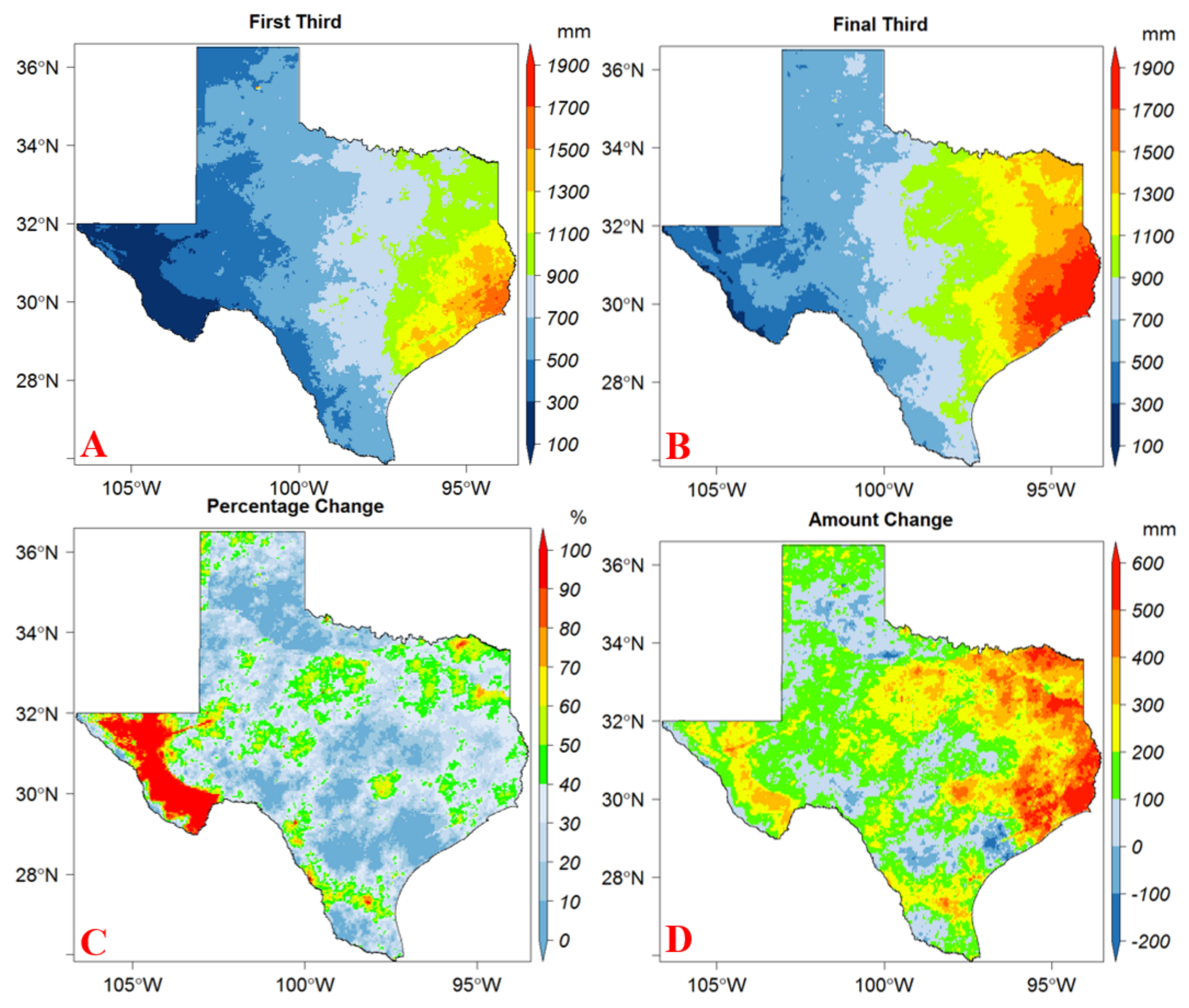
An initial investigation was conducted on the precipitation data to check if there was a significant trend in precipitation by comparing the first-third (2002–2007) and final-third (2014–2019) of the annual series. Figure 2A,B show the spatial distribution of the average precipitation of the first-third and the final-third. The difference between the two averages was more than 20%, indicating a significant increase over the study period. This increase was more pronounced in the wetter part of the state. The area receiving annual precipitation higher than 1500mm increased from 7000 km² to about 51,000 km², an increase by more than seven-fold. However, the general spatial pattern remained the same, with the northern coast of the Gulf being the wettest for the entire study period. Similarly, the western region received the lowest annual precipitation with the gradient moving in the west to east direction. The majority of the state (~60%) showed an increase of 25% in its annual precipitation in the final-third compared to the first-third of the time series (Figure 2C). The western region experienced the highest percentage increase reaching as high as 300% for some locations. When considering the amount of the precipitation increase, the state’s precipitation increased at an average of ~200 mm. The spatial distribution showed that the entire eastern region (bordering Louisiana) underwent an increase by more than 300 mm.

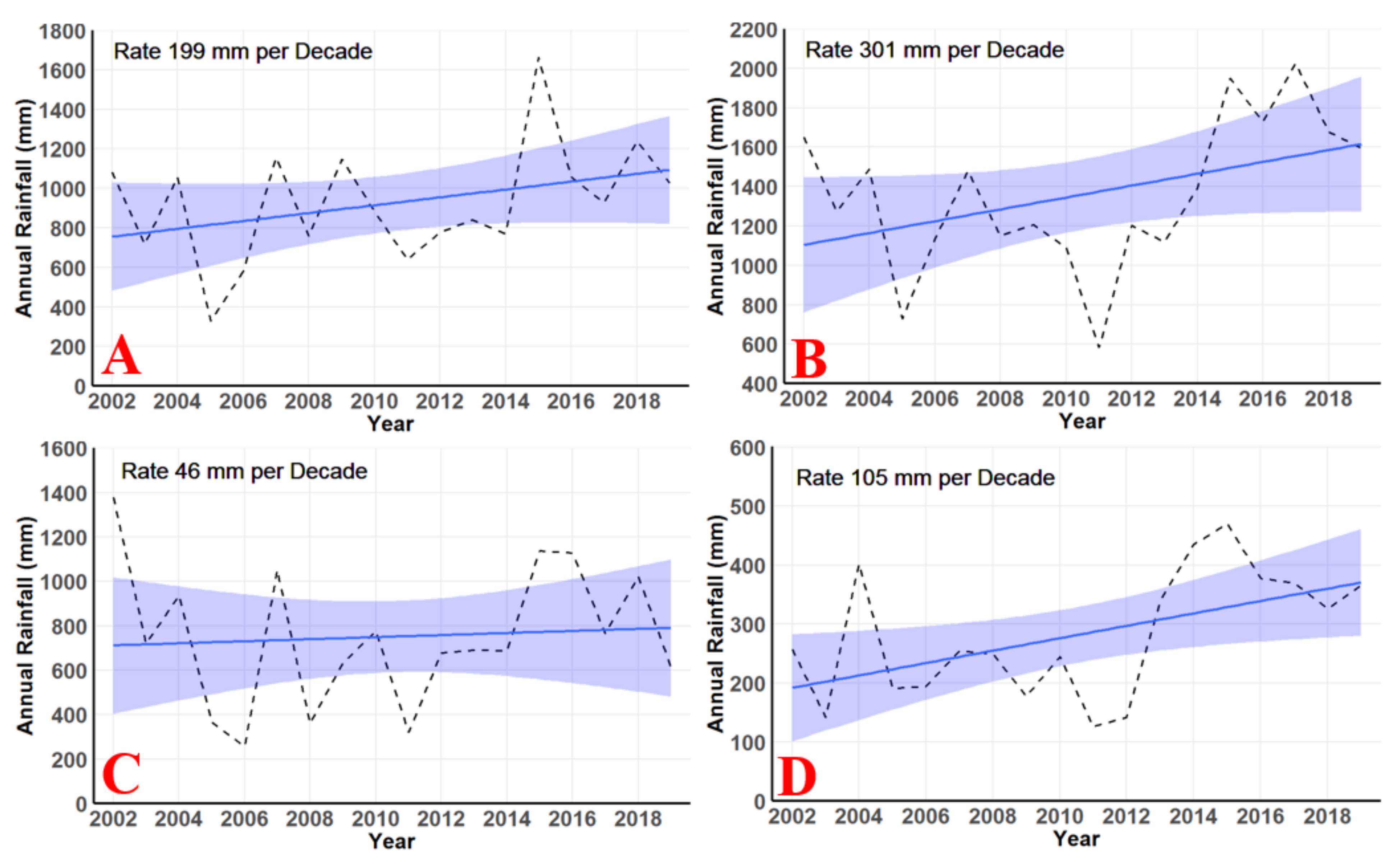
Further analysis was conducted to assess the trend of the annual precipitation in four of the major metropolitan areas of Texas: Dallas-Fort Worth, Houston, San Antonio, and El Paso, which are ranked first, second, third, and sixth in the state, respectively. More than 60% of the population of the state lives in these areas, and their locations (Figure 1) represent all regions of Texas. All of the metropolitan areas showed a steep trend with a rate ranging from 46 mm to 301 mm increase per decade (Figure 3). The Houston metropolitan area in coastal Texas had the highest rate of increase (Figure 3B), while San Antonio, which is located in the south-central region, had the lowest rate of increase (Figure 3C). Despite the steep increasing trend, all metropolitan areas showed a dip in their time-series around the period from 2011 to 2013.

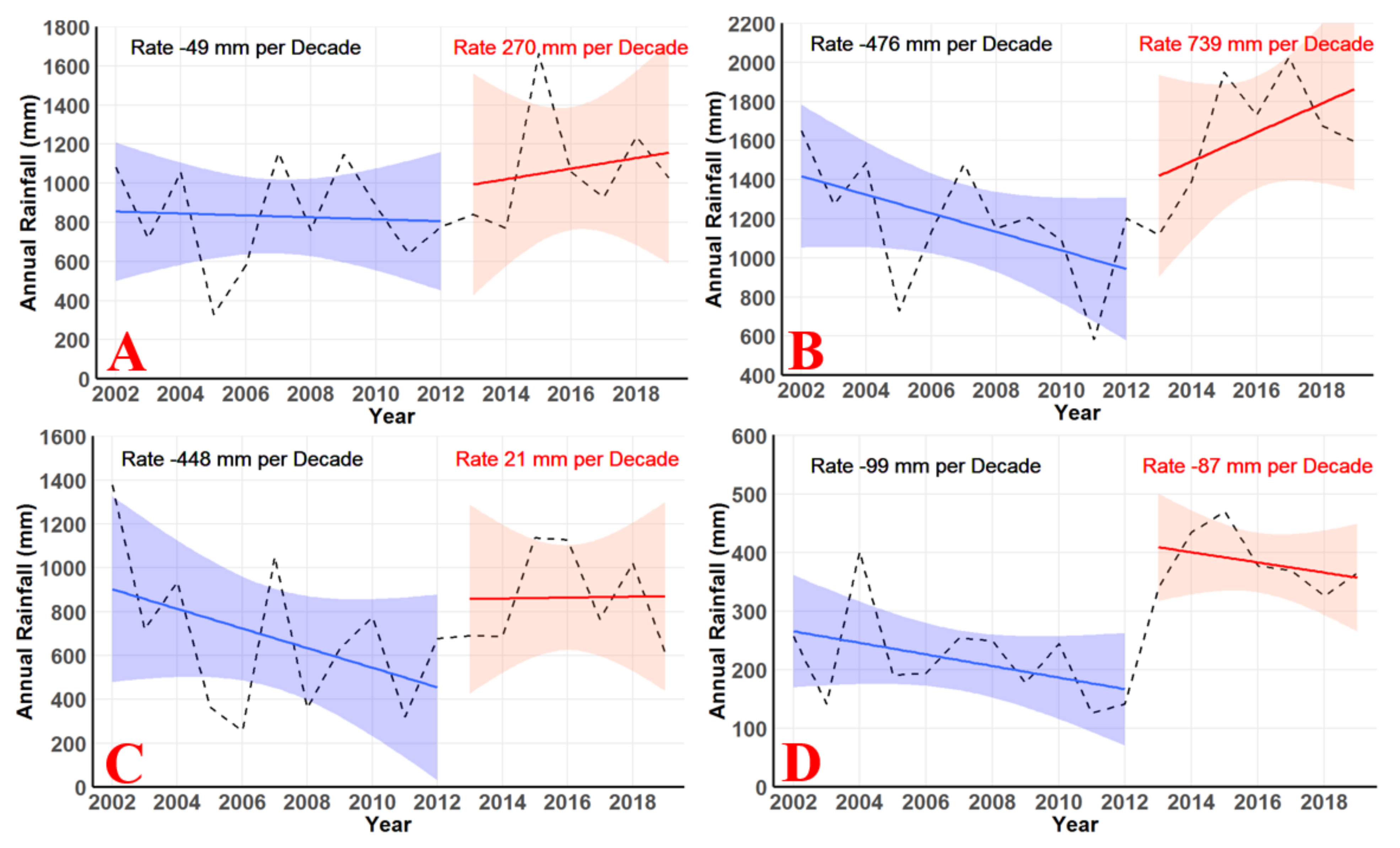
When the time series is split in 2013, the trends of the split series were quite different compared to the trend of the entire time series, as shown in Figure 4. For all metropolitan areas, the first period (2002–2013) had a declining trend in annual precipitation. Houston, San Antonio, and El Paso showed decreasing trends at rates of 476, 448, and 99 mm per decade, respectively. Dallas-Fort Worth metropolitan area showed fairly mild declining trends with a drop of 49 mm per decade. However, the second period showed conflicting trends among the metropolitan areas. Dallas-Fort Worth and Houston showed steep increasing trends at 739 and 270 mm per decade, respectively. On the contrary, El Paso experienced a steep decline in annual precipitation at about the same rate as before 2013. This highlights the fact that the annual precipitation in El Paso, which is located in the western tip of the state, only experienced an upward shift in the year 2012–2013. As for San Antonio, the trend line was almost flat with a slightly increasing trend. Another interesting observation is that as the distance from the Gulf of Mexico increased, the steepness of the trend line decreased and eventually became negative near El Paso. This agrees with previous studies that observed the strong influence of the Gulf of Mexico on precipitation magnitude and variability in Texas [28,46].

4.2. Seasonal Shifts

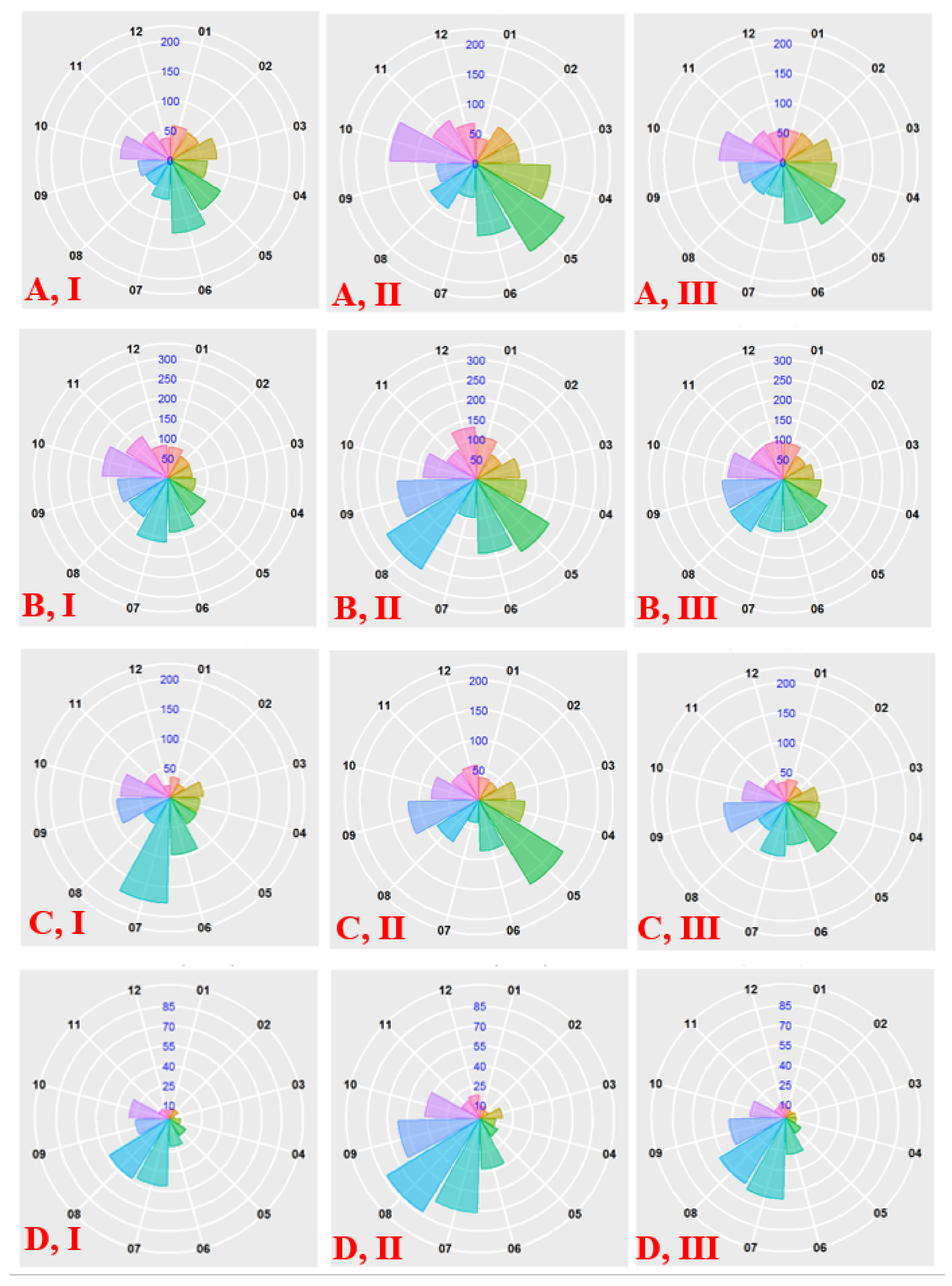
The average monthly accumulations for the first-third (2002–2007) and the last-third (2014–2019) of the study period were compared, as shown in Figure 5, through polar plots for the four metropolitan areas. This comparison helps identify shifts in the precipitation seasonality across the state. The last column (Figure 5III) shows the average monthly cumulative precipitation for the entire study period. For all four metropolitan areas, the average monthly cumulative precipitation showed a significant increase from the first-third to the last-third of the study period. In Dallas-Fort Worth, only one month (June) recorded an average of more than 100 mm in the first-third. However, four months recorded more than 100 mm with the highest about 170 mm (May) in the last-third. Moreover, the rainy season started one month earlier in the last third (Figure 5A). Similar to Dallas-Fort Worth, Houston also experienced a dramatic change in the monthly average with only two months (July and October) recording more than 150 mm in the first-third increasing to four in the last-third with as high as 250 mm in August. Monthly precipitation in Houston, the wettest metropolitan area, had two peaks as shown in Figure 5B. Precipitation appeared to peak earlier in the last-third of the study period. Another metropolitan area that showed a shift in the rainy season was San Antonio. The wettest month in the first-third was July with an average of around 175 mm, which became one of the driest months in the final-third with around 40 mm only. May, one of the driest months in the first-third, replaced July as the wettest month in the last-third with more than 150 mm. El Paso, the driest metropolitan area, showed an increase in the monthly precipitation for all months reaching as high as 85 mm in August in the last-third of the study period (Figure 5D). Overall, there was a shift in the rainy season, coming one month early in Dallas-Fort Worth and San Antonio, and an increase in the amount of rainfall experienced in all the metropolitan areas.

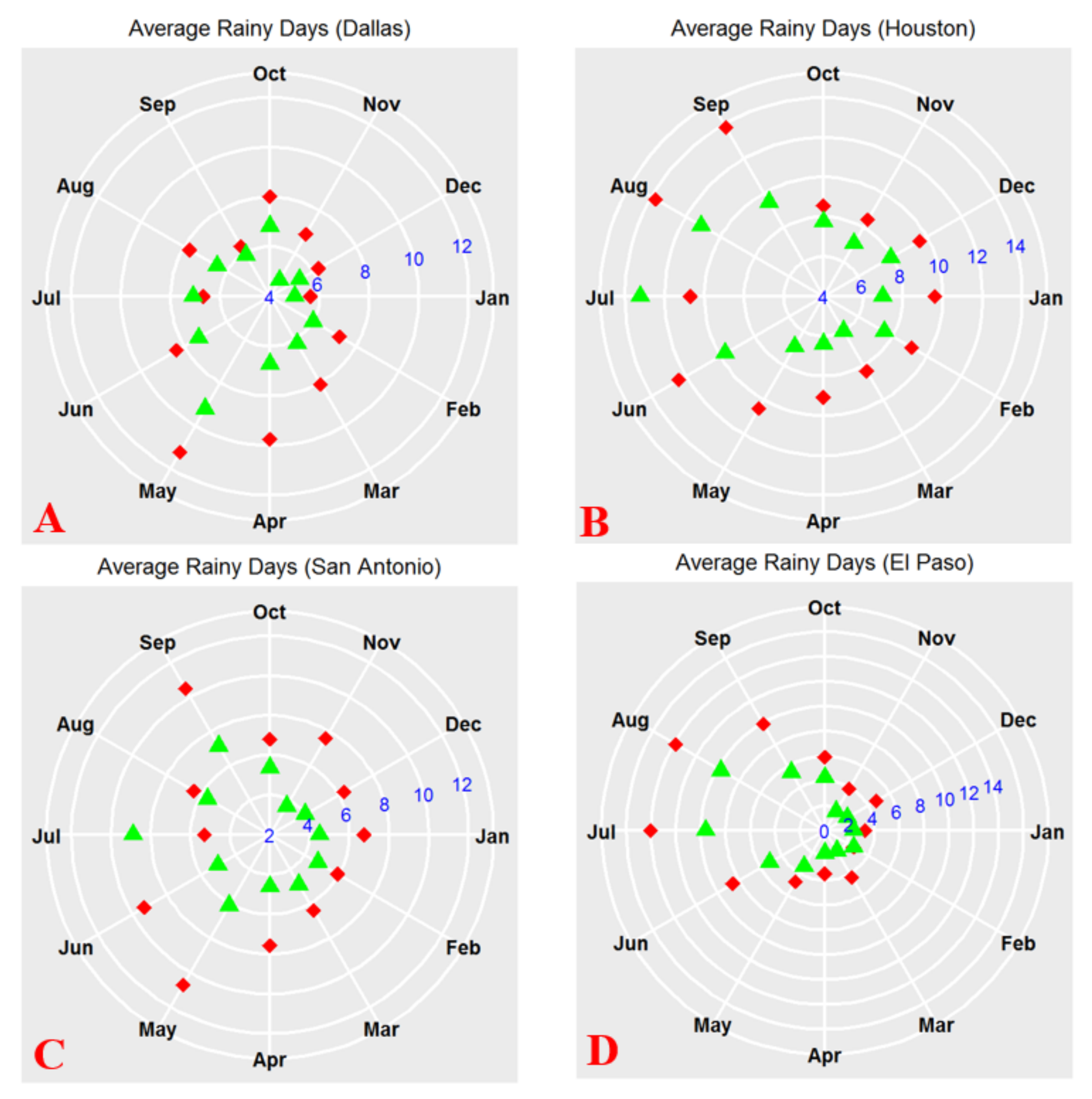
The seasonal change in precipitation in the metropolitan areas was also examined by computing the number of rainy days in a month before and after 2013. Overall, across the entire state, most of the months experienced an increase in the number of wet days after 2013 as shown in Figure 6. In Dallas-Fort Worth, the number of rainy days increased in all the months except July (Figure 6A). Similarly, in Houston and San Antonio, the month of July was the only month with fewer rainy days after 2013 than before 2013 (Figure 6B,C). The largest decrease in the number of rainy days for July was observed in San Antonio by about four days on average. This suggests that July became drier in the central and eastern parts of the state. El Paso showed the opposite effect in July. The rainy days increased by four days in July and August to 14 days for each month (Figure 6D). This was the highest number of rainy days in a month in all the metropolitan areas. This can be due to the different climatic controls that influence precipitation variabilities; El Paso is more affected by the activities in the Pacific Ocean, while other metropolitan areas are mostly affected by activities in the Gulf of Mexico.

4.3. Spatial Distribution of Shifts in Precipitation

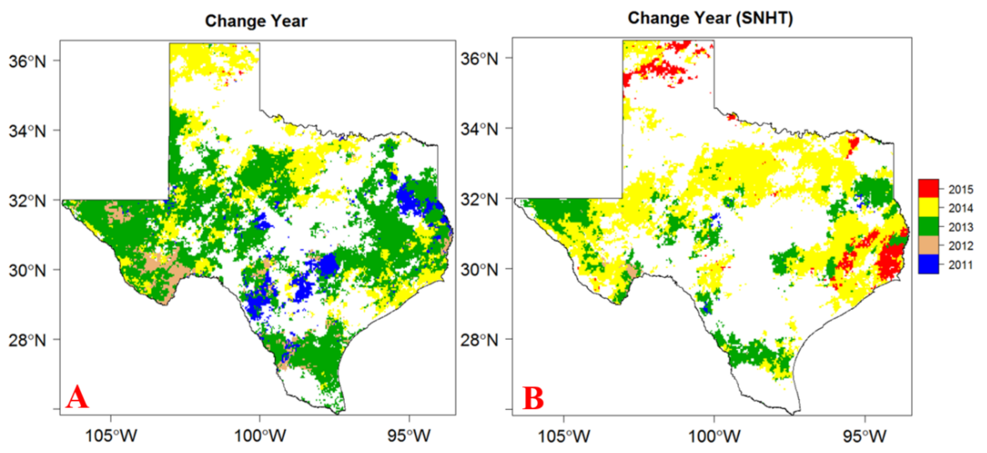
An investigation was conducted to determine the exact change point in the time series of the precipitation data, if any, with the statistical tests presented in Section 3.1 and Section 3.2. The decomposed monthly time series (without seasonal cycle) was used with a sample size of 216 months. The analysis was carried on all the 40,434 pixels across the state. The most common change point years were found to be between 2011 and 2015 with Pettitt’s test and Standard Normal Homogeneity Test (SNHT). When using the non-parametric test (Pettitt’s test), 60% of the state showed a significant change point that fell between 2011 and 2015 (Figure 7A). The most common change point years identified by Pettitt’s test were 2013 and 2014, collectively covering 50% of the state’s area, i.e., more than 80% of the area that showed a significant change point. Similarly, the SNHT test showed an area of more than 50% to have a significant change point for the years from 2013 to 2015. Around 80% of the area that showed a significant change point indicated that the change point occurred between 2013 and 2014 (Figure 7B). The results of this analysis are consistent with the results of the annual trend analysis carried in Section 4.1 based on the comparison of the first and last thirds of the precipitation time series.

4.4. Homogeneity of Precipitation

The tests described in Section 3.3 and Section 3.4 were used to statistically confirm whether the mean annual precipitation significantly changed over the study period. As described in Section 4.3, the time series was split at the beginning of the year 2013. Wilcoxon rank-sum test was used to find out whether the means of the two periods came from the same population. Using Student’s t-test, 65% of the state indicated that the means of the monthly precipitation data before and after 2013 were significantly different (Figure 8A). This result was also supported by the result of the non-parametric Wilcoxon rank test. More than three-quarters of the state of Texas showed that the monthly precipitation data before 2013 and after did not come from the same population at the significance level of 5% according to the Wilcoxon method (Figure 8B). Interestingly, 64% of the state indicated precipitation means before and after 2013 were significantly different by both tests. Most of the dry northern part of the state (Panhandle region) did not show a change in the mean precipitation according to both tests. The Panhandle region of Texas differed from the rest of the state in terms of precipitation variability and trends in a study conducted by Walsh [17]. This difference between the results of the two tests was mostly clustered over the central and the southern parts of the state.

4.5. Precipitation Trends

The three statistical tests described in Section 3.5, Section 3.6 and Section 3.7 were used to investigate the presence of a significant trend in precipitation before and after the change-point at the radar pixel scale. Theil-Sen’s slope test showed that around 30% of the state experienced a significant trend (positive or negative) before the year 2013. The majority of the areas with significant trends were located in the southeastern part near the Gulf of Mexico and the Panhandle region (Figure 9A). However, after 2013, only 2% of the area of the state showed a significant trend in precipitation (Figure 9B), mostly in the dryer parts of the state. When the trend test was applied to the entire time series (2002–2019), 30% of the state showed a significant trend (Figure 9C). However, the spatial pattern in Figure 9C is quite different from that of Figure 9A, showing areas with significant trends concentrated in the western part of the state and areas bordering the state of Louisiana (Figure 9C).

Another test that was used to assess the trend was the Seasonal Adjusted Mann-Kendall test, which is suitable for seasonally correlated data. The test detected a barely significant trend in the time series before and after 2013, as shown in small scattered green areas in Figure 10A,B. Before 2013 only 2%, and after 2013 less than 1%, of the total area showed a significant trend. However, when the entire time-series was tested, it showed a significant trend in more than 11% of the state. Almost all the areas that showed significant trends were located in the western region. This agrees with the results discussed in Section 4.1 (Figure 3D) when the change point is ignored.

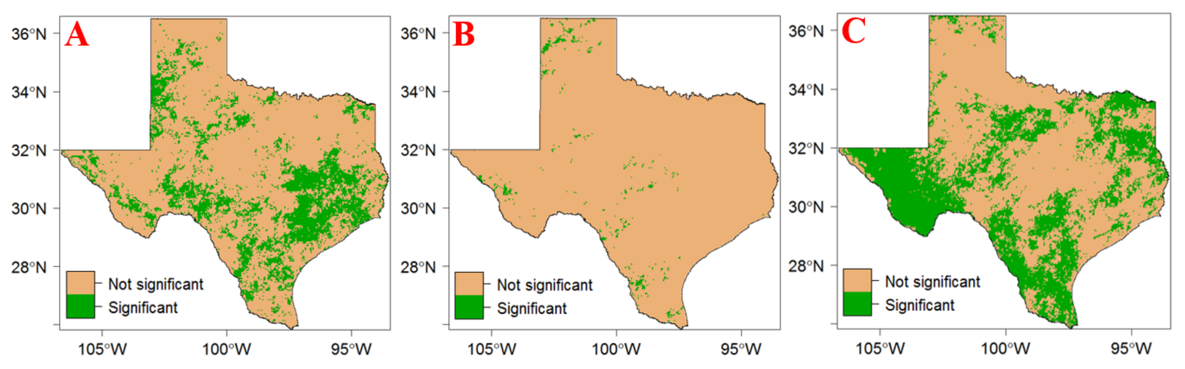
The last statistical test used was the non-parametric Cox and Stuart trend analysis test. The test showed a spatial pattern similar to the results of Theil-Sen’s slope test. In the period before 2013, around 23% of the state, mainly closer to the Gulf of Mexico, showed a significant trend (Figure 11A). However, after the change point, only 1.5% of the state showed a significant trend. Again, when the entire time series was considered, more than 36% of the state showed a significant trend in precipitation (Figure 11C). The majority of the areas that showed a significant trend in precipitation were located in the western and southern parts of the state.

The results of the three tests suggest the areas that experienced a significant trend in the period after 2013 (2013–2019) accounted for less than 2% of the state of Texas and were scattered within the state. The three tests also agreed that, when the entire time series was considered, a notable portion (~11%) of the state located in the western region showed a significant trend (Figure 9C, Figure 10C and Figure 11C). Furthermore, the same areas also showed a significant change-point in their precipitation time series around the years of 2013 and 2014 (Figure 7A,B).

4.6. Teleconnections with Climate Indices

The analysis described in the previous sections (Section 4.3 and Section 4.4) indicates that the precipitation experienced an upward shift in the year around 2013 across most of Texas. The trend analysis (Section 4.5) revealed that some areas did show a significant trend in precipitation before and after 2013. The next step was to try to find out whether this shift in the time series was related to major climate indices. The most common method is to check if there is a change in phase in a time series is by applying a cumulative sum of the index.

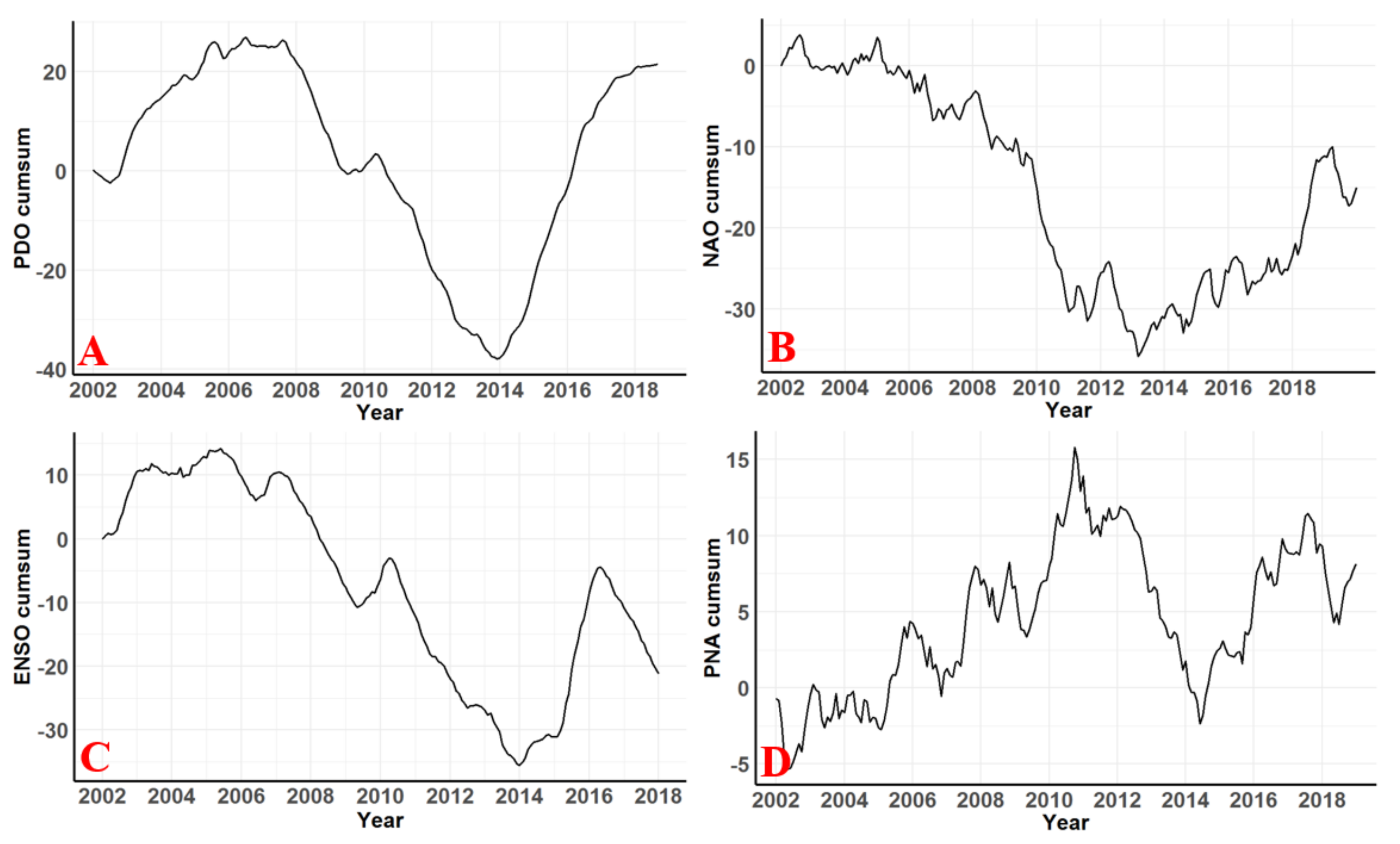
Four climatic indices showed a change in their phase around 2013 when a significant change-point was detected in the precipitation time-series for most of Texas (Figure 12). Previous studies have shown that the Pacific Decadal Oscillation (PDO) and the El Niño-Southern Oscillation (ENSO) indices had a significant influence on the variability of precipitation in the southern region of the US [22,23,24,47]. Both indices showed a clear change of phase in 2014 (Figure 12A,B), a year that showed a change-point in large areas of Texas (Figure 7A,B). The North Atlantic Oscillation index also showed a phase change in 2013 (Figure 12B), and lastly, the Pacific North American Index showed a change in phase shortly after 2014 (Figure 12D).

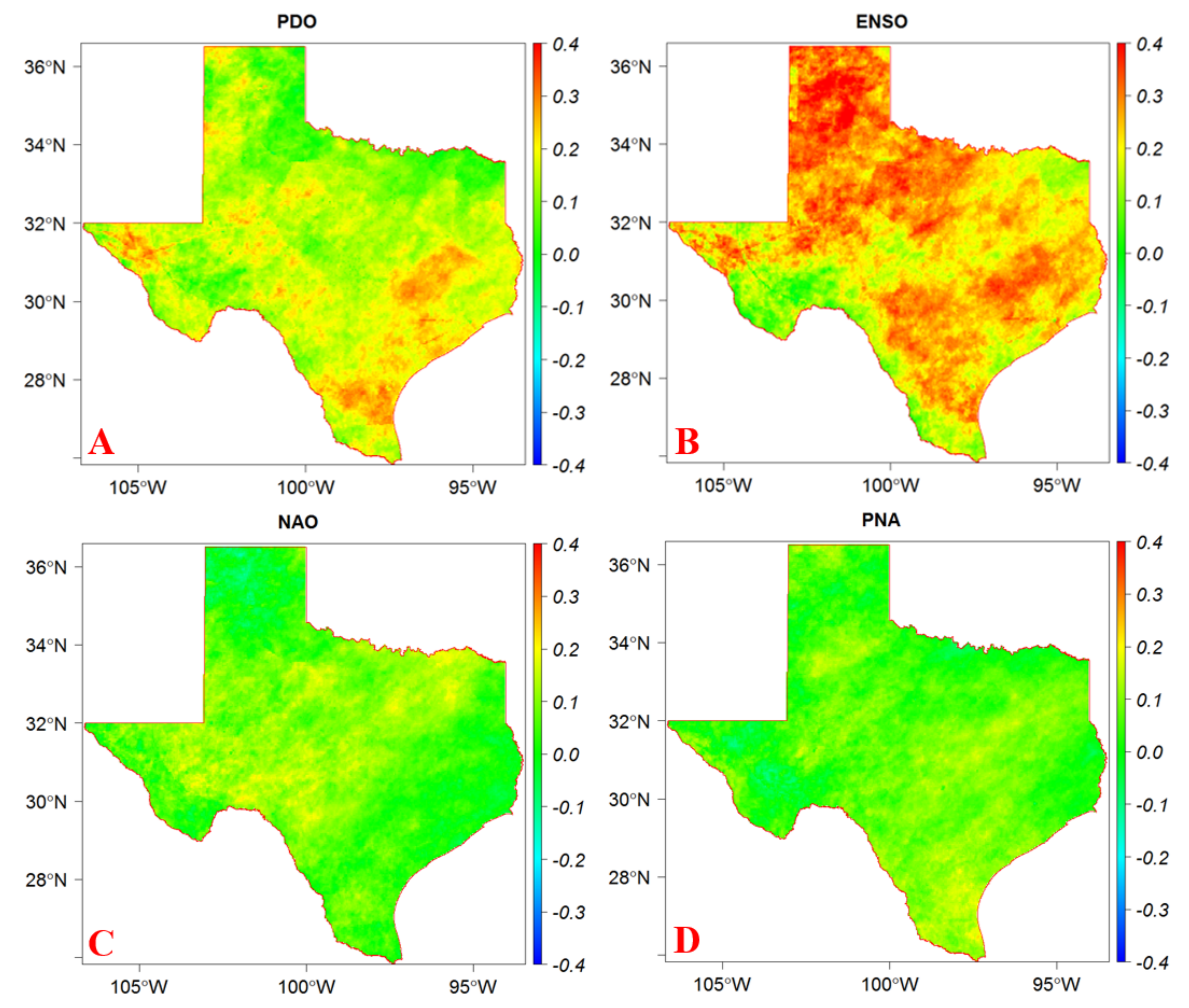
The spatial distribution of the correlation coefficient between the monthly precipitation data and the four climate indices at zero lag time is displayed in Figure 13. The climate index with the highest correlation coefficients was the ENSO index (Figure 13B). ENSO showed a correlation coefficient of more than 0.25 over around 46% of the state, especially in the Panhandle area and near the Gulf of Mexico. The Pacific Decadal Oscillation (PDO) also showed a slightly higher correlation coefficient in the area closer to the Gulf of Mexico (Figure 13A). In the case of PDO, only 5% of the state showed a correlation coefficient of more than 0.25. The other two climate indices (NAO and PNA) showed a small correlation coefficient across the state with a very small spatial variability. This suggests that the most influential climatic index in the state of Texas was the ENSO precipitation index. Nevertheless, PDO also has showed strong correlations with the precipitation across large areas of the state.

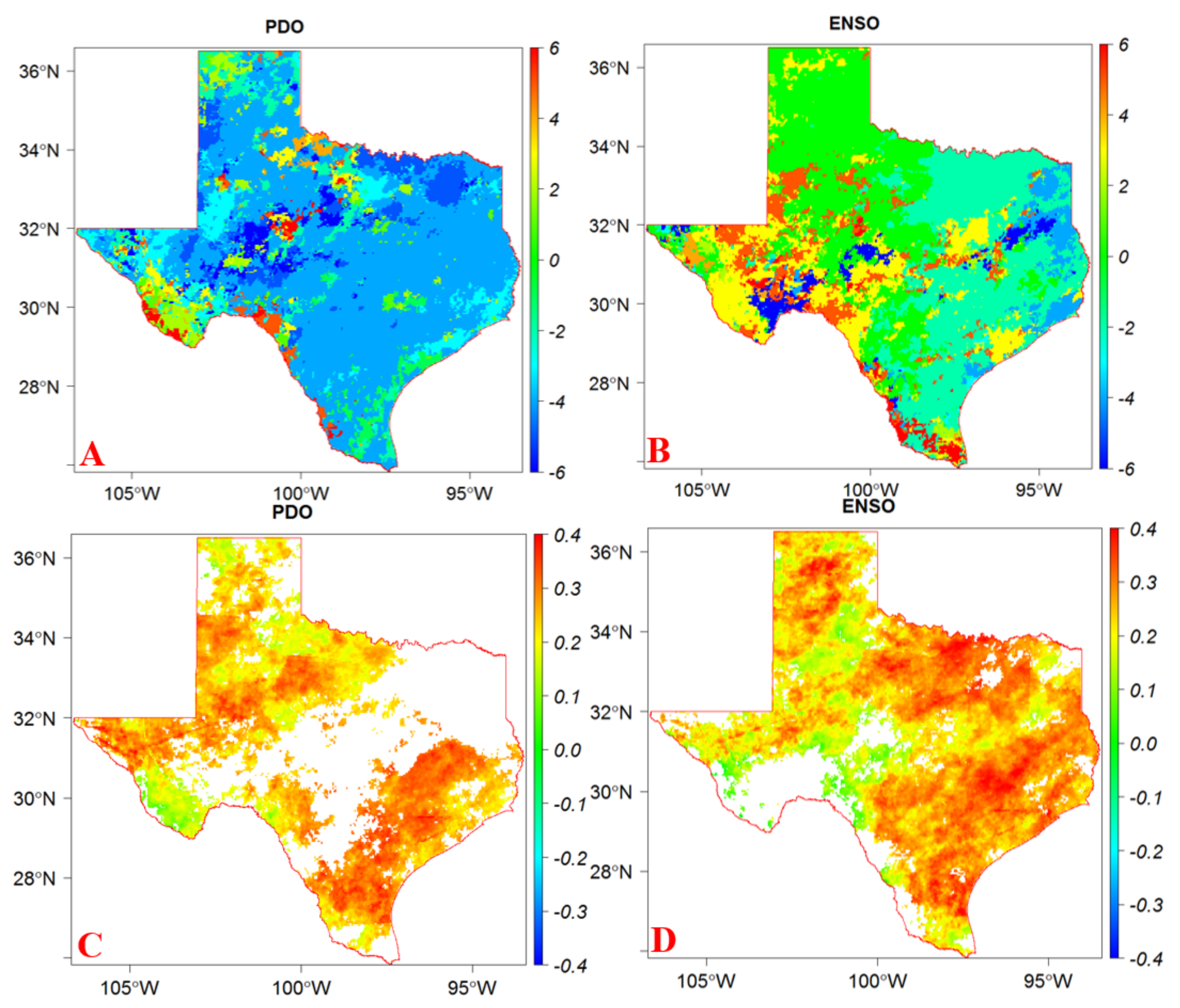
The correlation of the two main climatic indices with precipitation was analyzed further to identify the value of the lag with the highest correlation. The highest correlation between the PDO and precipitation was found to be at a value of 4-month lag, i.e., PDO leading the monthly precipitation. Around 60% of the state showed the highest correlation with PDO at a 4-month lag, as shown in Figure 14A. However, the highest correlation with the ENSO was found at lag values of 0 and 2 months leading (Figure 14B). The area closer to the Gulf of Mexico (around 30% of the area of the state) showed a higher correlation with ENSO at 2 months leading lag (Figure 14B). The POD correlation coefficient was higher at a 4-month lag throughout the state, especially in the Panhandle area (Figure 14C). The 2-month leading correlation showed a higher correlation in the eastern areas near the Gulf of Mexico (Figure 14 D). The spatial distribution of the significant correlation with ENSO was higher for the eastern part of the state at a 2-month lag (Figure 14D). About 82% of the state showed a statistically significant correlation with the ENSO at a 2-month lag. However, the other two climate indices (NAO and PNA) only showed a significant correlation in less than a quarter of the state for all lags.

5. Summary and Conclusions

Detailed statistical analysis was conducted on the monthly and annual precipitation over the state of Texas using Stage-IV radar data with a 4km × 4km spatial resolution and over the time frame that spans from 2002 to 2019. The average precipitation in the state of Texas showed a dramatic increase by more than 20% between the first-third (2002–2007) and the last-third (2014–2019) of the study period. This increase was more pronounced in the wetter parts of the state. The area receiving annual precipitation higher than 1500 mm increased from 7000 km² to about 51,000 km², an increase by more than seven-fold. The annual precipitation indicated an increasing trend in all four major metropolitan areas with as high as 301 mm per decade in Houston and as low as 46 mm per decade in the case of San Antonio. However, when the time series data were split in 2013, all metropolitan areas exhibited a decreasing trend before 2013.

The monthly precipitation was found to be significantly higher in the last-third of the study period in all four metropolitan areas. For example, in Dallas-Fort Worth, there was only one month (June) that recorded more than 100 mm in the first-third of the study period. However, four months recorded more than 100 mm with the highest about 170 mm (May) in the last-third of the study period. Similar to Dallas-Fort Worth, Houston had also experienced a dramatic change in the monthly average with only two months (July and October) recording more than 150 mm in the first-third increasing to four the last-third with as high as 250 mm/month in August.

The most common change-point years identified by Pettitt’s test were 2013 and 2014, collectively detected in 50% of the state’s area, i.e., more than 80% of the area that showed significant change point. Similarly, the SNHT test showed an area of more than 50% to have had a significant change point for the years from 2013 to 2015. Test of homogeneity of the data before and after the change-point (2013) was carried to investigate whether the samples (before and after 2013) belonged to the same population. More than three-quarters of the state of Texas showed that the monthly precipitation data before and after 2013 did not come from the same population at the significance level of 5% according to the Wilcoxon method. Using Student’s t-test, 65% of the state indicated that the means of the monthly precipitation data before and after 2013 were significantly different. Furthermore, 64% of the state indicated precipitation means before and after 2013 were significantly different by both tests. The spatial distribution revealed that the Panhandle region (dry northern part) of the state did not show a change in the mean precipitation according to both tests. The Panhandle region of Texas also differed from the rest of the state in terms of precipitation variability and trends in a study conducted by Walsh [17].

The spatial pattern of the trend analysis was found to be similar in three statistical significance tests. The tests suggest that the state did not experience a significant trend in precipitation after 2013 according to the three tests (only less than 2% of the state indicated a significant trend). However, when the entire time series was tested for trends, the western region of the state exhibited a positive increasing trend for all three tests. Furthermore, these areas also showed a significant change-point in their precipitation time series around the years 2013 and 2014.

Lastly, the time-series was investigated for possible correlation with the major climatic indices to establish the presence of teleconnections. Pacific Decadal Oscillation (PDO), North Atlantic Oscillation, El Niño-Southern Oscillation (ENSO) precipitation index, and Pacific North American Index were considered for the correlation analysis because they showed a change in their phase around 2013 when a significant change-point was detected in the precipitation time-series for most of Texas. ENSO had the highest correlation coefficient with the precipitation of Texas at a 2-month lag. The monthly precipitation and ENSO showed a statistically significant correlation in 82% of the state with a 2-month lag. Precipitation also exhibited a significant correlation with POD at a 4-month lag in over 60% of the state. The other two climate indices (NAO and PNA) showed a weak correlation coefficient across the entire state with a very small spatial variability for all lags. The results suggest that the most influential climate index in the state of Texas was the ENSO precipitation index. Nevertheless, PDO also showed strong correlations with the precipitation across large areas of the state. In summary, the precipitation of Texas was strongly affected by the ENSO and PDO at a lag of 2 months and 4 months, respectively. There was a significant upward shift in the precipitation of the state that was overwhelmingly experienced in 2013. A shift like this in a time-series can lead to the detection of an apparent increasing trend if not treated separately.

The study results suggest that the monthly precipitation did not show a significant trend across the entire state after the shift in 2013. However, the water withdrawal from groundwater for irrigation purposes soared by around 18% from 2015 to 2018, which is an increase of 11.1 billion cubic meters according to a report from the state’s water board. This shows the extent of the divergence of the withdrawal and the recharge trends. The outcome from this study will shed light on the status of the precipitation’s spatiotemporal variability across the state and guide adjustment of the current water resources management practices accordingly. Moreover, the spatial component of the analysis results can inform a diverse water resource management practice suited to the state’s very diverse climate. The results of such an analysis can also be used to enhance both the spatial and temporal resolutions of low spatial, low temporal, historical, and projected precipitation time series (i.e., downscaling and interpolation).

The relatively short length of the dataset has to be mentioned because, for climatic analysis, a time series of at least 30 years is typically recommended. In this case, only 18 years (2002–2019) of data were used in the analysis. The discontinuity in the data due to the operational processing at the radar site may have slightly affected the results, especially in the western region. The frequencies described are contingent upon the radar precipitation threshold used and the NEXRAD products’ accuracy. Nonetheless, the information gleaned from this analysis will be useful for many applications, including natural hazard mitigation, flood resilience studies, water security assessment, and water resources planning and management.

References

- Trenberth, K.E.; Zhang, Y.; Gehne, M. Intermittency in Precipitation: Duration, Frequency, Intensity, and Amounts Using Hourly Data. J. Hydrometeorol. 2017, 18, 1393–1412. [Google Scholar] [CrossRef] [Green Version]
- Ouarda, T.; Charron, C.; Kumar, K.N.; Marpu, P.; Ghedira, H.; Molini, A.; Khayal, I. Evolution of the rainfall regime in the United Arab Emirates. J. Hydrol. 2014, 514, 258–270. [Google Scholar] [CrossRef] [Green Version]
- Ullah, S.; You, Q.; Ullah, W.; Ali, A. Observed changes in precipitation in China-Pakistan economic corridor during 1980–2016. Atmos. Res. 2018, 210, 1–14. [Google Scholar] [CrossRef]
- Zarenistanak, M.; Dhorde, A.G.; Kripalani, R.H. Trend analysis and change point detection of annual and seasonal precipitation and temperature series over southwest Iran. J. Earth Syst. Sci. 2014, 123, 281–295. [Google Scholar] [CrossRef]
- Villarini, G.; Smith, J.A.; Baeck, M.L.; Marchok, T.; Vecchi, G.A. Characterization of rainfall distribution and flooding associated with U.S. landfalling tropical cyclones: Analyses of Hurricanes Frances, Ivan, and Jeanne (2004). J. Geophys. Res. Space Phys. 2011, 116. [Google Scholar] [CrossRef]
- Linsley, R.; Franzini, J.; Freyberg, D.; Tchobanoglous, G. Water Resources Engineering; McGraw-Hill: New York, NY, USA, 1992; p. 841. [Google Scholar]
- Habib, E.H.; Meselhe, E.A.; Aduvala, A.V. Effect of Local Errors of Tipping-Bucket Rain Gauges on Rainfall-Runoff Simulations. J. Hydrol. Eng. 2008, 13, 488–496. [Google Scholar] [CrossRef]
- Wang, X.; Xie, H.; Sharif, H.; Zeitler, J. Validating NEXRAD MPE and Stage III precipitation products for uniform rainfall on the Upper Guadalupe River Basin of the Texas Hill Country. J. Hydrol. 2008, 348, 73–86. [Google Scholar] [CrossRef]
- Krajewski, W.; Smith, J. Radar hydrology: Rainfall estimation. Adv. Water Resour. 2002, 25, 1387–1394. [Google Scholar] [CrossRef]
- Nelson, B.R.; Prat, O.P.; Seo, D.-J.; Habib, E. Assessment and Implications of NCEP Stage IV Quantitative Precipitation Estimates for Product Intercomparisons. Weather. Forecast. 2016, 31, 371–394. [Google Scholar] [CrossRef]
- Qiao, L.; Hong, Y.; Chen, S.; Zou, C.B.; Gourley, J.J.; Yong, B. Performance assessment of the successive Version 6 and Version 7 TMPA products over the climate-transitional zone in the southern Great Plains, USA. J. Hydrol. 2014, 513, 446–456. [Google Scholar] [CrossRef]
- Omranian, E.; Sharif, H.O.; Tavakoly, A.A. How Well Can Global Precipitation Measurement (GPM) Capture Hurricanes? Case Study: Hurricane Harvey. Remote. Sens. 2018, 10, 1150. [Google Scholar] [CrossRef] [Green Version]
- Sharif, R.B.; Habib, E.H.; ElSaadani, M. Evaluation of Radar-Rainfall Products over Coastal Louisiana. Remote. Sens. 2020, 12, 1477. [Google Scholar] [CrossRef]
- Prat, O.P.; Nelson, B.R. Evaluation of precipitation estimates over CONUS derived from satellite, radar, and rain gauge data sets at daily to annual scales (2002–2012). Hydrol. Earth Syst. Sci. 2015, 19, 2037–2056. [Google Scholar] [CrossRef] [Green Version]
- Furl, C.; Ghebreyesus, D.; Sharif, H.O. Assessment of the Performance of Satellite-Based Precipitation Products for Flood Events across Diverse Spatial Scales Using GSSHA Modeling System. Geosciences 2018, 8, 191. [Google Scholar] [CrossRef] [Green Version]
- Cho, Y.; Engel, B.A. NEXRAD Quantitative Precipitation Estimations for Hydrologic Simulation Using a Hybrid Hydrologic Model. J. Hydrometeorol. 2016, 18, 25–47. [Google Scholar] [CrossRef]
- Walsh, J.E.; Richman, M.B. Seasonality in the Associations between Surface Temperatures over the United States and the North Pacific Ocean. Mon. Weather. Rev. 1981, 109, 767–783. [Google Scholar] [CrossRef] [Green Version]
- Lyons, S.W. Spatial and Temporal Variability of Monthly Precipitation in Texas. Mon. Weather. Rev. 1990, 118, 2634–2648. [Google Scholar] [CrossRef] [Green Version]
- Ghebreyesus, D.; Sharif, H.O. Spatio-Temporal Analysis of Precipitation Frequency in Texas Using High-Resolution Radar Products. Water 2020, 12, 1378. [Google Scholar] [CrossRef]
- Rahmani, V.; Hutchinson, S.L.; Jr, J.A.H.; Hutchinson, J.M.S.; Anandhi, A. Analysis of temporal and spatial distribution and change-points for annual precipitation in Kansas, USA. Int. J. Clim. 2015, 35, 3879–3887. [Google Scholar] [CrossRef]
- Karl, T.R.; Knight, R.W. Secular Trends of Precipitation Amount, Frequency, and Intensity in the United States. Bull. Am. Meteorol. Soc. 1998, 79, 231–241. [Google Scholar] [CrossRef]
- Molnár, P.; Ramírez, J.A. Recent Trends in Precipitation and Streamflow in the Rio Puerco Basin. J. Clim. 2001, 14, 2317–2328. [Google Scholar] [CrossRef]
- Roswintiarti, O.; Niyogi, D.S.; Raman, S. Teleconnections between tropical pacific sea surface temperature anomalies and North Carolina precipitation anomalies during El Niño events. Geophys. Res. Lett. 1998, 25, 4201–4204. [Google Scholar] [CrossRef]
- Boyles, R.P.; Raman, S. Analysis of climate trends in North Carolina (1949–1998). Environ. Int. 2003, 29, 263–275. [Google Scholar] [CrossRef] [Green Version]
- Liu, L.; Hong, Y.; Hocker, J.E.; Shafer, M.A.; Carter, L.M.; Gourley, J.J.; Bednarczyk, C.N.; Yong, B.; Adhikari, P. Analyzing projected changes and trends of temperature and precipitation in the southern USA from 16 downscaled global climate models. Theor. Appl. Clim. 2012, 109, 345–360. [Google Scholar] [CrossRef]
- Nielsen-Gammon, J.W. The Changing Climate of Texas. In The Impact of Global Warming on Texas; University of Texas Press: Austin, TX, USA, 2011; pp. 39–68. [Google Scholar]
- Nielsen-Gammon, J.W.; Banner, J.L.; Cook, B.I.; Tremaine, D.M.; Wong, C.I.; Mace, R.E.; Gao, H.; Yang, Z.; Gonzalez, M.F.; Hoffpauir, R.; et al. Unprecedented Drought Challenges for Texas Water Resources in a Changing Climate: What Do Researchers and Stakeholders Need to Know? Earth’s Future 2020, 8. [Google Scholar] [CrossRef]
- Asquith, W.H. Depth-Duration Frequency of Precipitation for Texas; US Geological Survey: Reston, VA, USA, 1998; Volume 98, p. 4044. [Google Scholar]
- Alvarez, E.C.; Plocheck, R. Texas Almanac 2012–2013; Texas A&M University Press: College Station, TX, USA, 2011. [Google Scholar]
- Fulton, R.A.; Breidenbach, J.P.; Seo, D.-J.; Miller, D.A.; O’Bannon, T. The WSR-88D Rainfall Algorithm. Weather. Forecast. 1998, 13, 377–395. [Google Scholar] [CrossRef]
- Seo, D.-J.; Breidenbach, J.P. Real-Time Correction of Spatially Nonuniform Bias in Radar Rainfall Data Using Rain Gauge Measurements. J. Hydrometeorol. 2002, 3, 93–111. [Google Scholar] [CrossRef] [Green Version]
- Lin, Y.; Mitchell, K.E. 1.2 the NCEP stage II/IV hourly precipitation analyses: Development and applications. In Proceedings of the 19th Conference Hydrology American Meteorological Society, San Diego, CA, USA, 9–13 January 2005. [Google Scholar]
- Verstraeten, G.; Poesen, J.; Demarée, G.; Salles, C. Long-term (105 years) variability in rain erosivity as derived from 10-min rainfall depth data for Ukkel (Brussels, Belgium): Implications for assessing soil erosion rates. J. Geophys. Res. Space Phys. 2006, 111. [Google Scholar] [CrossRef]
- Alexandersson, H. A homogeneity test applied to precipitation data. J. Clim. 1986, 6, 661–675. [Google Scholar] [CrossRef]
- Rodionov, S.N. A brief overview of the regime shift detection methods. Large-Scale Disturbances (Regime Shifts) and Recovery in Aquatic Ecosystems: Challenges for Management toward Sustainability. In Proceedings of the UNESCO-ROSTE/BAS Workshop on Regime Shifts, Varna, Bulgaria, 14–16 June 2005; Velikova, V., Chipev, N., Eds.; pp. 17–24. [Google Scholar]
- Nurdin, S.; Mustapha, M.A.; Lihan, T. The relationship between sea surface temperature and chlorophyll-a concentration in fisheries aggregation area in the archipelagic waters of spermonde using satellite images. In Proceedings of the Universiti Kebangsaan Malaysia, Faculty of Science and Technology 2013 Postgraduate Colloquium, Selangor, Malaysia, 3–4 July 2013; AIP Publishing: Melville, NY, USA, 2013; Volume 1571, pp. 466–472. [Google Scholar]
- Wehbe, Y.; Temimi, M.; Ghebreyesus, D.T.; Milewski, A.; Norouzi, H.; Ibrahim, E. Consistency of precipitation products over the Arabian Peninsula and interactions with soil moisture and water storage. Hydrol. Sci. J. 2018, 63, 408–425. [Google Scholar] [CrossRef]
- Theil, H. A rank-invariant method of linear and polynomial regression analysis, Part III. Nederlandsche Akad. van Wetenschappen Proc. 1950, 58, 1397–1412. [Google Scholar]
- Sen, P.K. Estimates of the regression coefficient based on Kendall’s tau. J. Am. Statistic. Assoc. 1968, 63, 1379–1389. [Google Scholar] [CrossRef]
- Dinpashoh, Y.; Jhajharia, D.; Fakheri-Fard, A.; Singh, V.P.; Kahya, E. Trends in reference crop evapotranspiration over Iran. J. Hydrol. 2011, 399, 422–433. [Google Scholar] [CrossRef]
- Jhajharia, D.; Dinpashoh, Y.; Kahya, E.; Choudhary, R.R.; Singh, V.P. Trends in temperature over Godavari River basin in Southern Peninsular India. Int. J. Clim. 2014, 34, 1369–1384. [Google Scholar] [CrossRef]
- Vousoughi, F.D.; Dinpashoh, Y.; Aalami, M.T.; Jhajharia, D. Trend analysis of groundwater using non-parametric methods (case study: Ardabil plain). Stoch. Environ. Res. Risk Assess. 2012, 27, 547–559. [Google Scholar] [CrossRef]
- Hirsch, R.M.; Slack, J.R.; Smith, R.A. Techniques of trend analysis for monthly water quality data. Water Resour. Res. 1982, 18, 107–121. [Google Scholar] [CrossRef] [Green Version]
- Libiseller, C.; Grimvall, A. Performance of partial Mann-Kendall tests for trend detection in the presence of covariates. Environmetrics 2002, 13, 71–84. [Google Scholar] [CrossRef]
- Cox, D.R.; Stuart, A. Some quick sign tests for trend in location and dispersion. Biometrika 1955, 42, 80–95. [Google Scholar] [CrossRef] [Green Version]
- Larkin, T.J.; Bomar, G.W. Climatic Atlas of Texas; Texas Department of Water Resources: Austin, TX, USA, 1983. [Google Scholar]
- Joseph, J.F.; Falcon, H.E.; Sharif, H.O. Hydrologic Trends and Correlations in South Texas River Basins: 1950–2009. J. Hydrol. Eng. 2013, 18, 1653–1662. [Google Scholar] [CrossRef]
Figure 1.
The study area including the nine major aquifers, major metropolitan areas of Texas, and the average annual precipitation from NEXt-generation Weather RADar (NEXRAD) Stage-IV (2002–2019).
Figure 2.
Spatial distribution of the average annual precipitation in the (A) first-third (2002–2007), (B) last-third of the study period (2014–2019), (C) percentage change (100 × (Final − First)/First), and (D) the amount of change in annual precipitation (Final–First).
Figure 3.
Annual precipitation time series and their trends for (A) Dallas-Fort Worth, (B) Houston, (C) San Antonio, and (D) El Paso metropolitan areas. The blue shade represents the 95% confidence interval of the trend line.
Figure 4.
Annual precipitation time series of the major metropolitan areas of Texas and their trend for (A) Dallas-Fort Worth, (B) Houston, (C) San Antonio, and (D) El Paso. The blue and red shades represent the 95% confidence interval of the trend line.
Figure 5.
Average monthly cumulative precipitation for the first and last third of the study period in the metropolitan areas of (A) Dallas-Fort Worth, (B) Houston, (C) San Antonio, and (D) El Paso. First-third (2002–2012) in column I, the last-third (2013–2019) in column II, and the entire period in column III.
Figure 6.
Polar plots showing the number of rainy days of the months before (green triangle) and after 2013 (red diamond) in (A) Dallas-Fort Worth, (B) Houston, (C) San Antonio, and (D) El Paso.
Figure 7.
Areas showing significant change-points and their change-point years using (A) Pettitt’s test and (B) the Standard Normal Homogeneity Test (SNHT).
Figure 8.
Areas with and without significantly different means and similar means before and after 2013 using (A) Student’s t-test and (B) Wilcoxon Rank Sum test.
Figure 9.
The spatial distribution of the precipitation trends based on Theil-Sen’s slope test for the period (A) before 2013 (2002–2012) and (B) after (2013–2019), and (C) for the entire study period.
Figure 10.
The spatial distribution of the precipitation trends based on the Correlated Seasonal Mann-Kendall test for the period (A) before 2013 (2002–2012) and (B) after 2013 (2013–2019), and (C) for the entire study period.
Figure 11.
The spatial distribution of the precipitation trends based on Cox and Stuart test for the period (A) before 2013 (2002–2012) and (B) after 2013 (2013–2019), and (C) for the entire study period.
Figure 12.
Cumulative sum of the major climate indices that show a change in phase around 2013: (A) Pacific Decadal Oscillation (PDO), (B) North Atlantic Oscillation (NAO), (C) El Niño-Southern Oscillation (ENSO) precipitation index, and (D) Pacific North American (PNA).
Figure 13.
Spatial distributions of the correlation coefficient without any lag between the monthly precipitation and the (A) Pacific Decadal Oscillation (PDO), (B) North Atlantic Oscillation (NAO), (C) El Niño-Southern Oscillation (ENSO) precipitation index, and (D) Pacific North American (PNA) indices.
Figure 14.
Spatial distributions of the value of the lag with the highest correlation in the (A) Pacific Decadal Oscillation (PDO), and (B) El Niño-Southern Oscillation (ENSO) climatic indices and the spatial distribution of the significant correlation of precipitation and (C) PDO and (D) ENSO indices.
Publisher’s Note: MDPI stays neutral with regard to jurisdictional claims in published maps and institutional affiliations. |
© 2021 by the authors. Licensee MDPI, Basel, Switzerland. This article is an open access article distributed under the terms and conditions of the Creative Commons Attribution (CC BY) license (https://creativecommons.org/licenses/by/4.0/).
Share and Cite
MDPI and ACS Style
Ghebreyesus, D.; Sharif, H.O. Time Series Analysis of Monthly and Annual Precipitation in The State of Texas Using High-Resolution Radar Products. Water 2021, 13, 982. https://0-doi-org.brum.beds.ac.uk/10.3390/w13070982
AMA Style
Ghebreyesus D, Sharif HO. Time Series Analysis of Monthly and Annual Precipitation in The State of Texas Using High-Resolution Radar Products. Water. 2021; 13(7):982. https://0-doi-org.brum.beds.ac.uk/10.3390/w13070982
Chicago/Turabian StyleGhebreyesus, Dawit, and Hatim O. Sharif. 2021. "Time Series Analysis of Monthly and Annual Precipitation in The State of Texas Using High-Resolution Radar Products" Water 13, no. 7: 982. https://0-doi-org.brum.beds.ac.uk/10.3390/w13070982
Note that from the first issue of 2016, this journal uses article numbers instead of page numbers. See further details here.