
Solution Selection from a Pareto Optimal Set of Multi-Objective Reservoir Operation via Clustering Operation Processes and Objective Values


Abstract
:1. Introduction
2. Methodology
2.1. Mei–Wang Fluctuation Similarity Measure
- is the index used to describe the difference in quantitative variation between and . It is calculated with Equation (2):where is the ordinate of the point , is the ordinate of the point , is the sequence number, N is the length of the process, and and are the means of and , respectively.
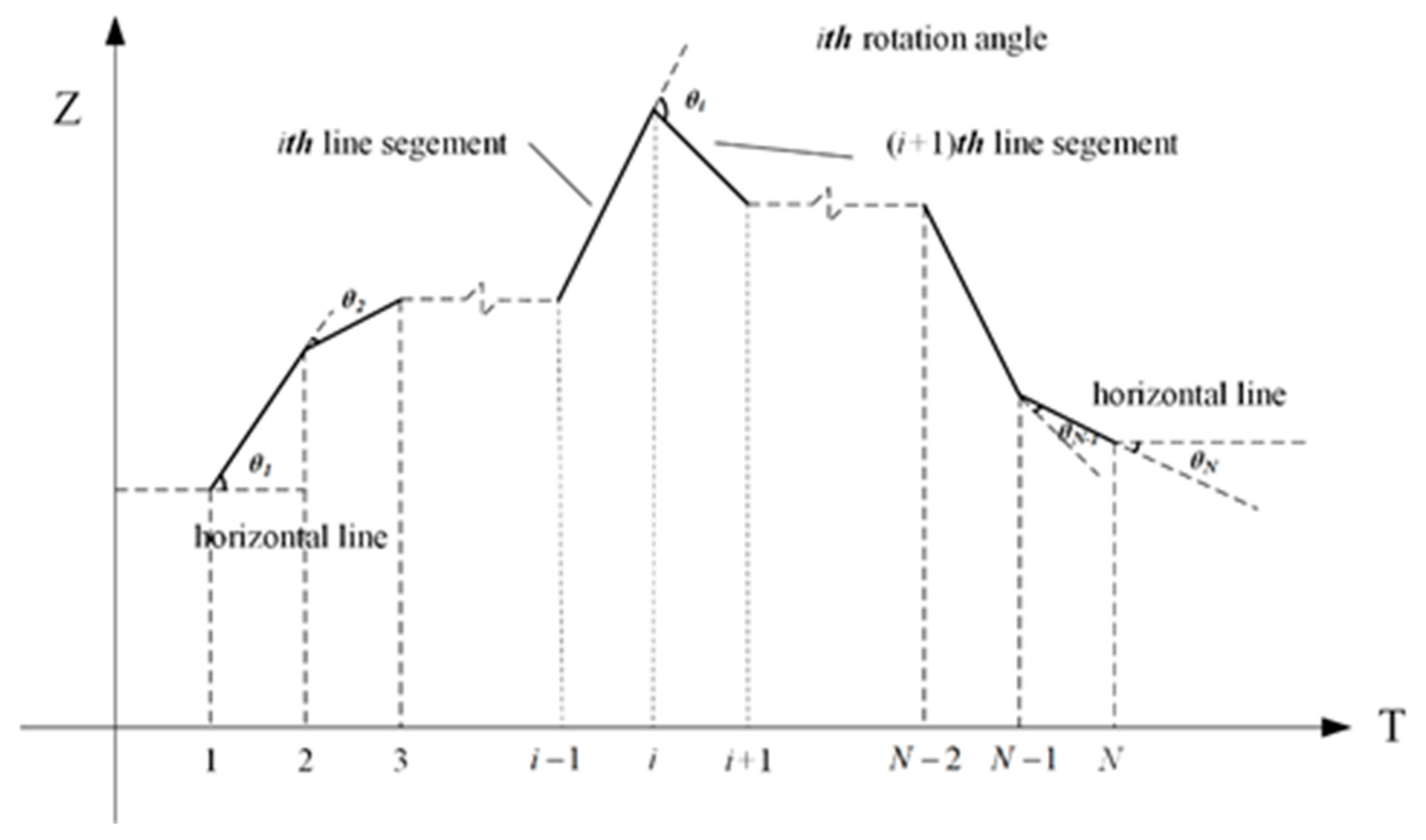
- is an index describing the difference between two processes in terms of contour variations. It is calculated with Equations (3)–(5):where is the angle between two line segments of and is the angle between two line segments of . The rotation angle and line segment of a process are shown in Figure 1. is selected as an example, and for or , is the rotation angle between the first line segment and a horizontal line, is the rotation angle between the last line segment and a horizontal line, and is the slope of the line segment, which is defined by Equation (5).
- The MWFSM between and is calculated with Equation (6) as follows:where is the index of the MWFSM method.
2.2. Clustering by Fast Search and Find of Density Peaks
- Calculate distance matrix via MWFSM.
- Sort in ascending order, assign the top 2% of the data column to .
- Calculate local density according to Equation (7) for each data point in .
- Calculate distance from the nearest larger density point according to Equations (8) and (9) for each data point in .
- Calculate the decision value according to Equation (10) for each data point in .
- Sort in ascending order and record the new order.
- Construct the decision value graph where points are represented as with the ascending order in Step 6.
- Select the points of the large γ values as cluster centers according to the decision value graph.
- Allocate the remaining points following the principle of proximity.
2.3. Clustering-Based Solution Selection Method
- The DPC method is applied to set and obtains clusters of decision processes.
- The clusters generated in step 1 are ranked by size, and the decision cluster is denoted as , and the decision cluster with the largest membership is denoted as .
- An operation pattern set consisting of the solutions corresponding to the centers of the decision clusters is generated.
- The k-means algorithm is employed to cluster set and obtain objective value clusters.
- The objective value clusters are ranked in descending order, and the cluster is denoted as , and the set with the largest membership is denoted as .
- The intersection of and is considered. If the intersection set is not empty, it is denoted as . If the intersection set is empty, the intersection of and the next objective cluster is determined. This process is repeated until the intersection set is no longer empty, which is then denoted as .
- The decision process with the minimum accumulative similarity in set is identified and recommended.
- The selected solution and the operation pattern set are provided to DMs.
2.4. Multi-Objective Optimization Model
2.4.1. Objective Functions
2.4.2. Constraints
- The water balance is expressed aswhere is the average storage of the cascade reservoir during the period, is the inflow of the cascade reservoir during the period, and is the outflow rate of the cascade reservoir during the period; is the duration.
- The outflow constraint is expressed aswhere is the inflow of the cascade reservoir, which is equal to the sum of the outflow of the cascade reservoir and the local inflow during the period.
- The power output constraint is given bywhere and are the minimum and maximum output power levels, respectively, of the plant during the period, and is the average output power of the plant during the period.
- The storage volume constraint is expressed aswhere and are the lower and upper bounds, respectively, of the water level of the dam during the period.
- The boundary condition limit is given bywhere and are the water levels of the cascade reservoir during the first and last periods, respectively, and is the initial water level of the dam, which is given in the case study.
3. Case Study
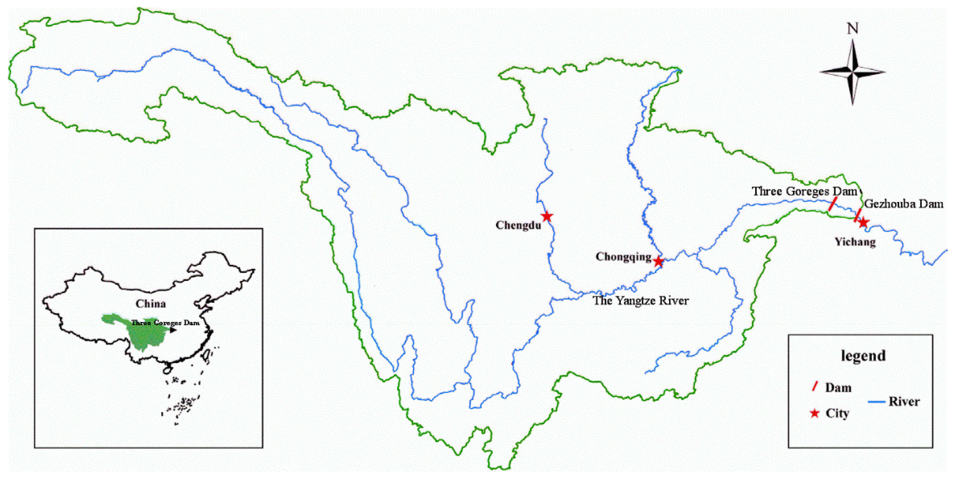
3.1. Study Area
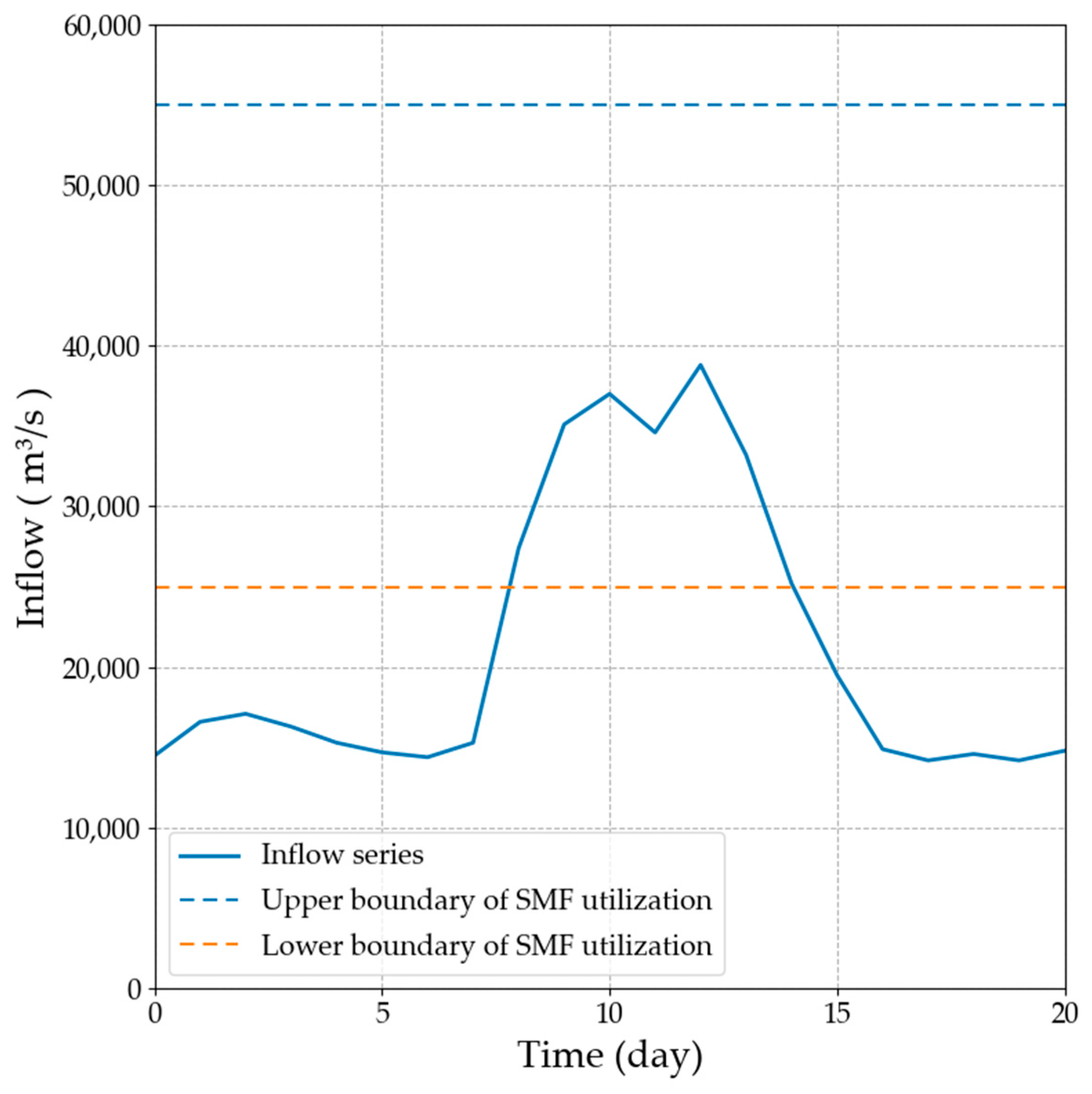
3.2. Input Data
4. Results and Discussion
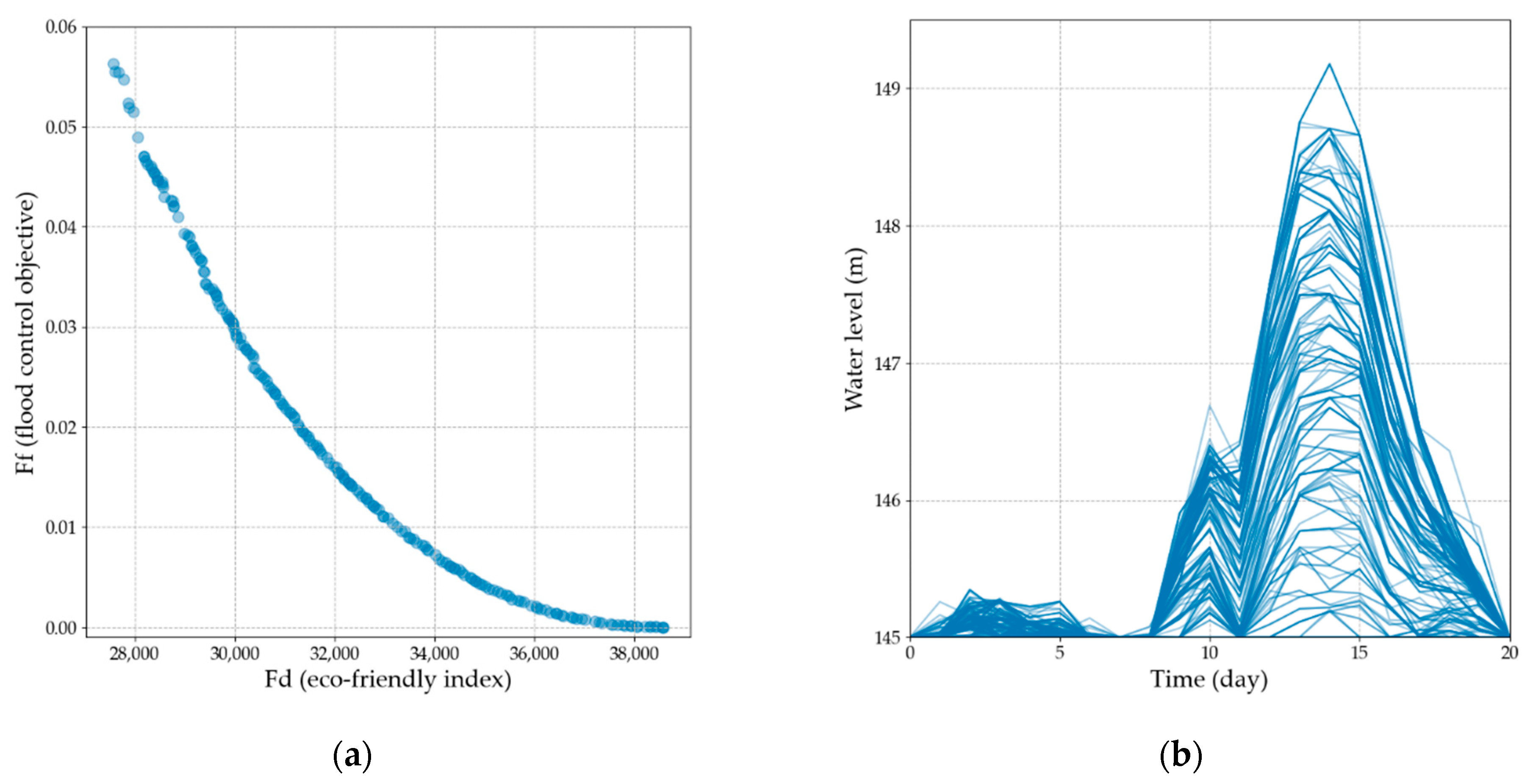
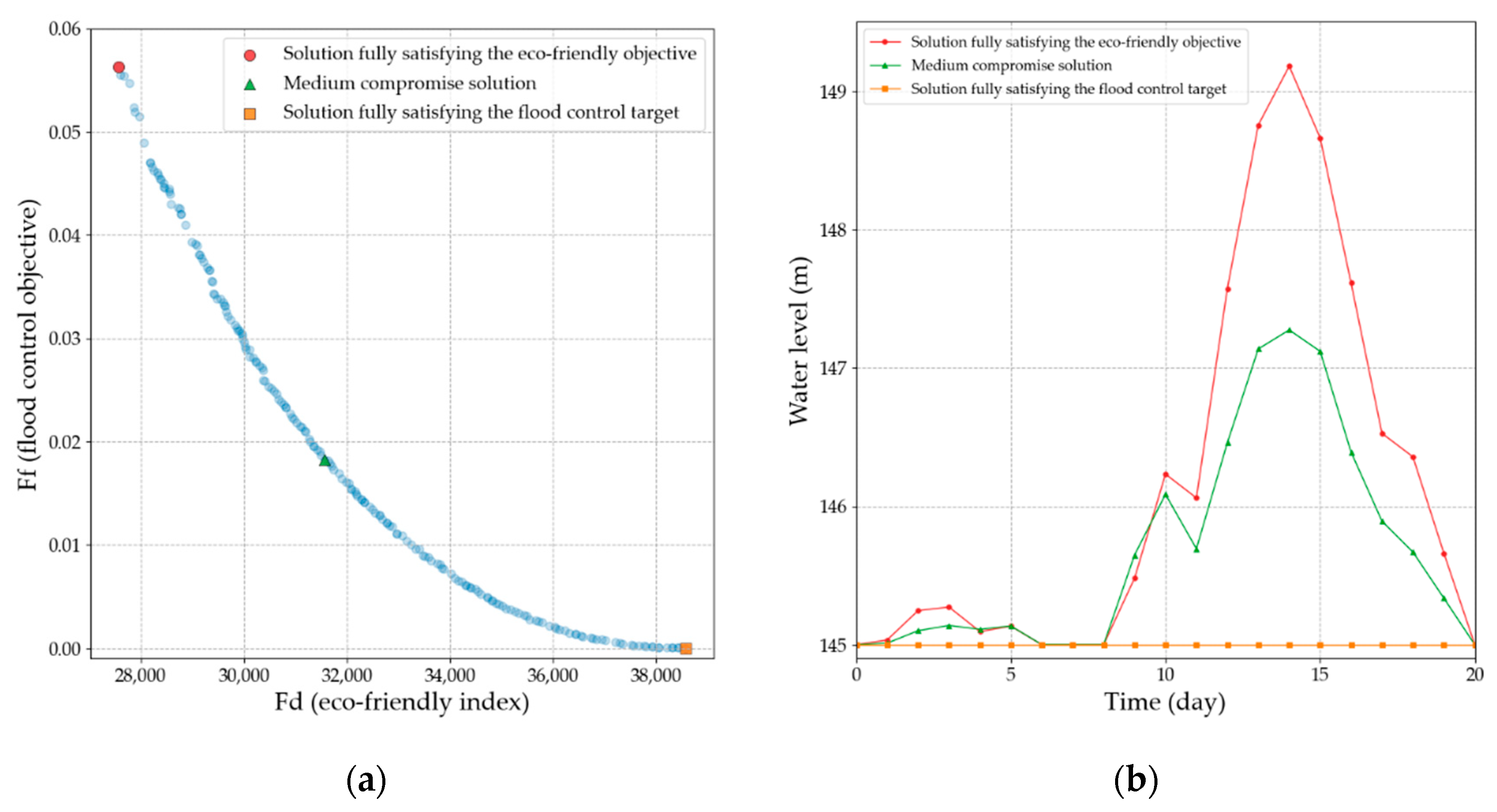
4.1. NSGA-II Output and Traditional Analysis of Pareto Set
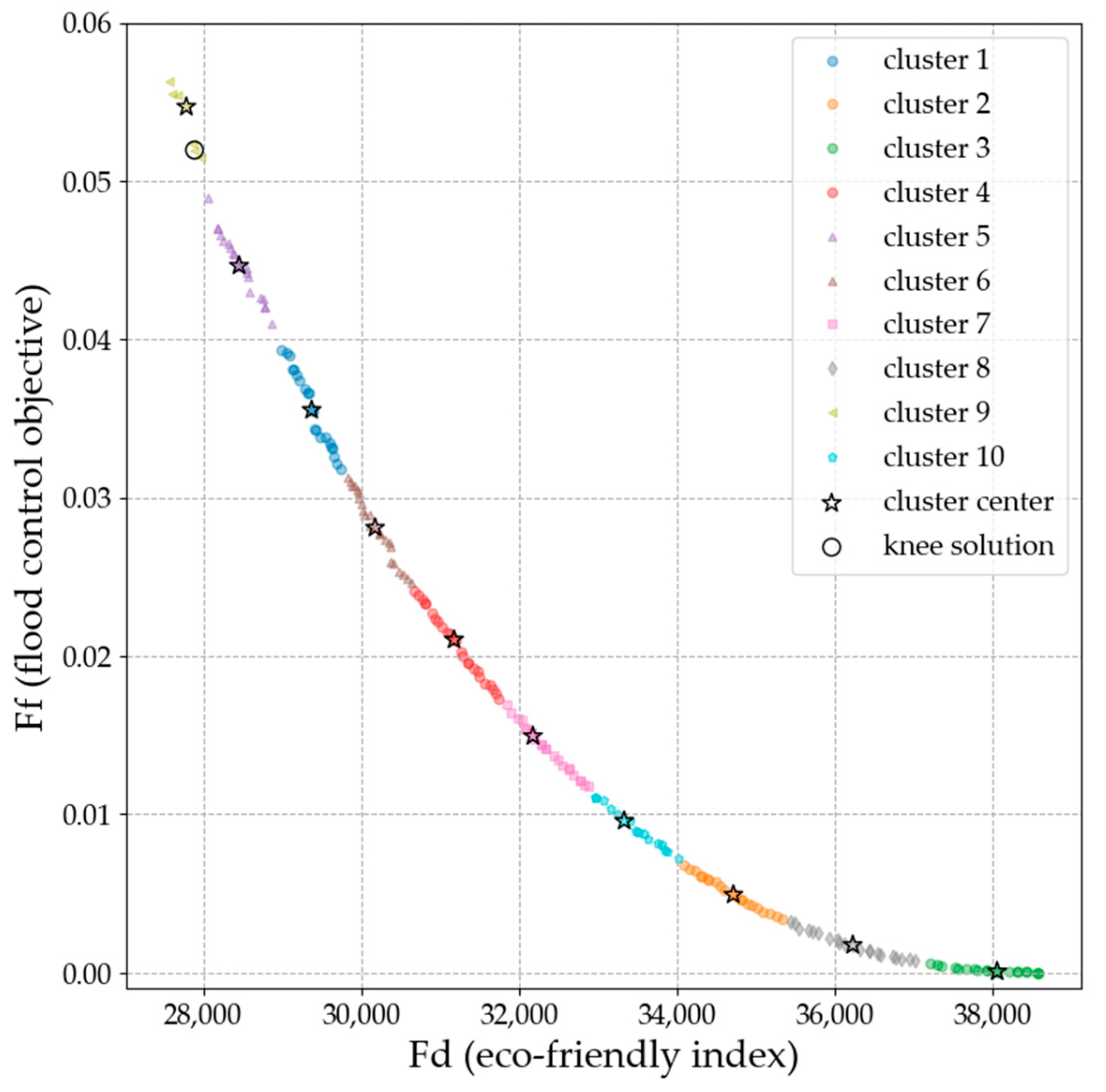
4.2. Clustering of the Trade-Off Frontier
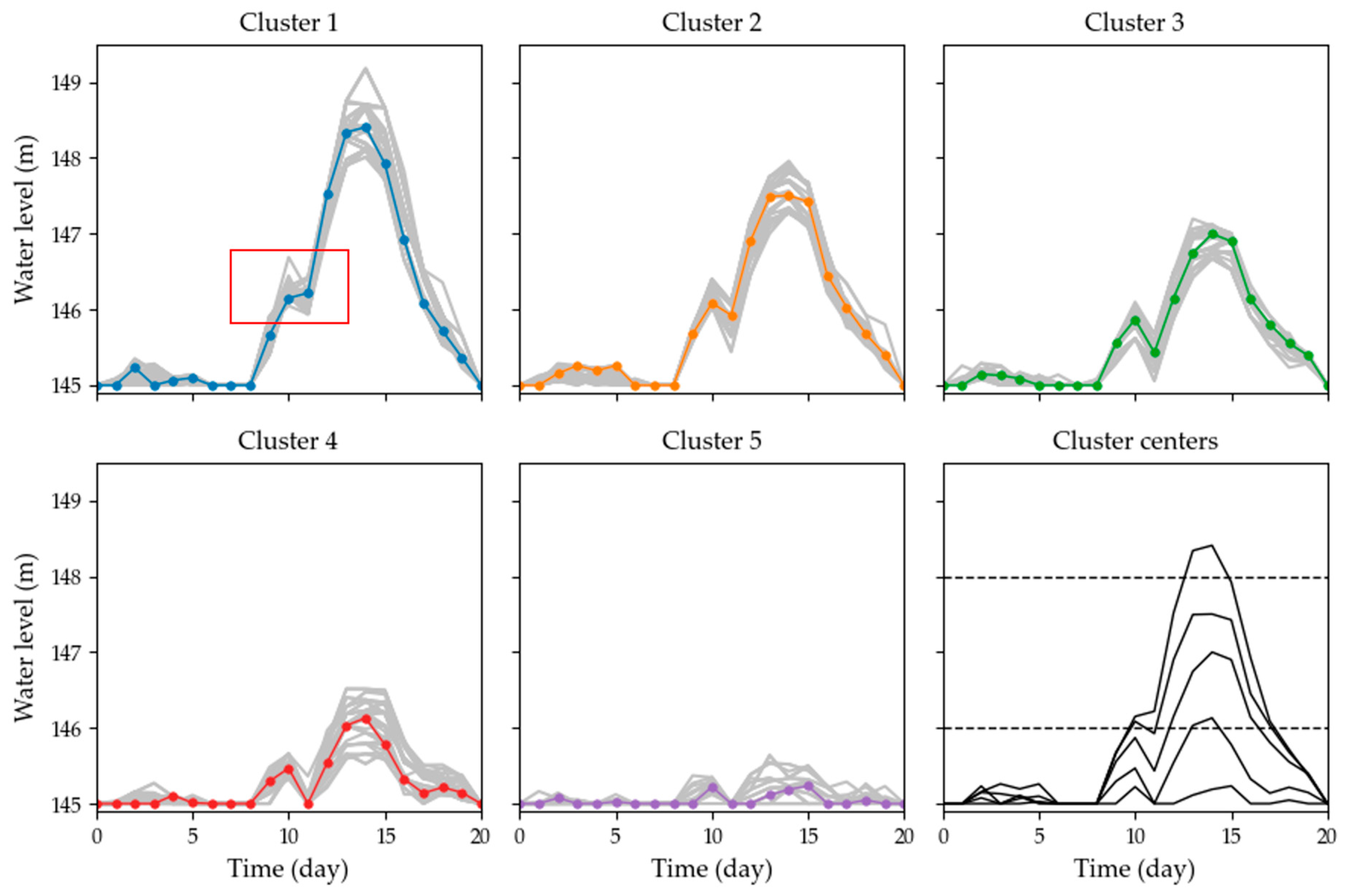
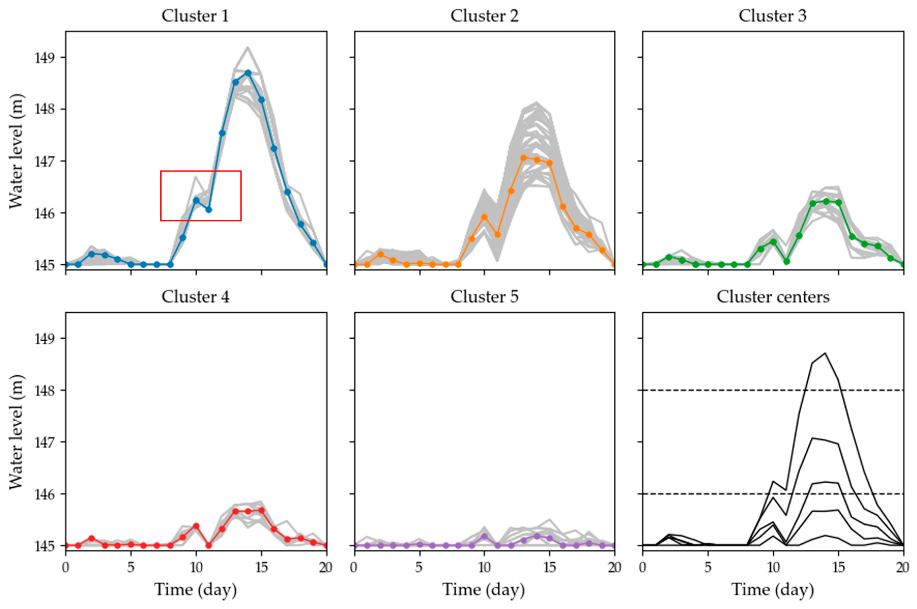
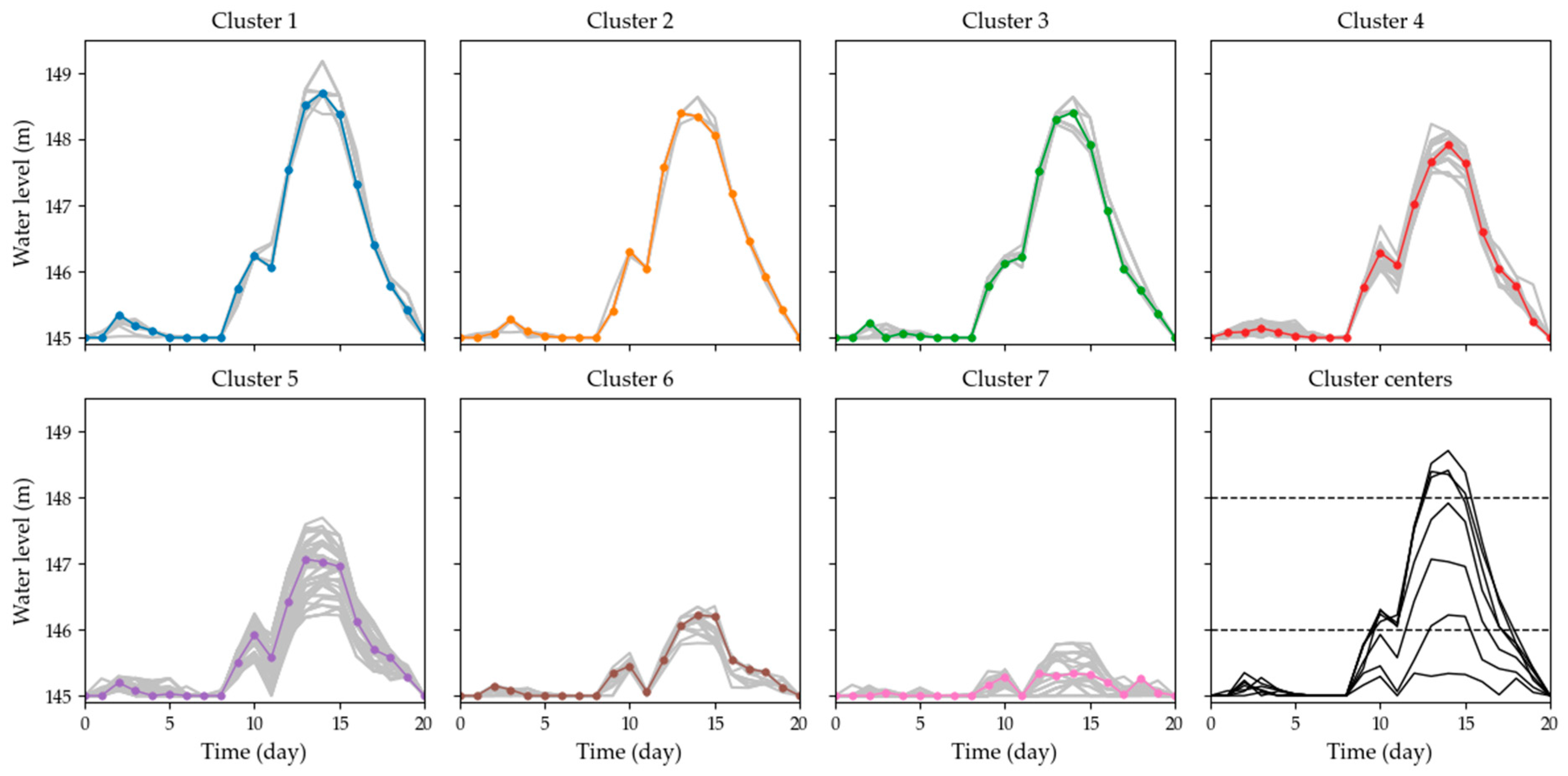
4.3. Clustering of the Reservoir Operation Processes
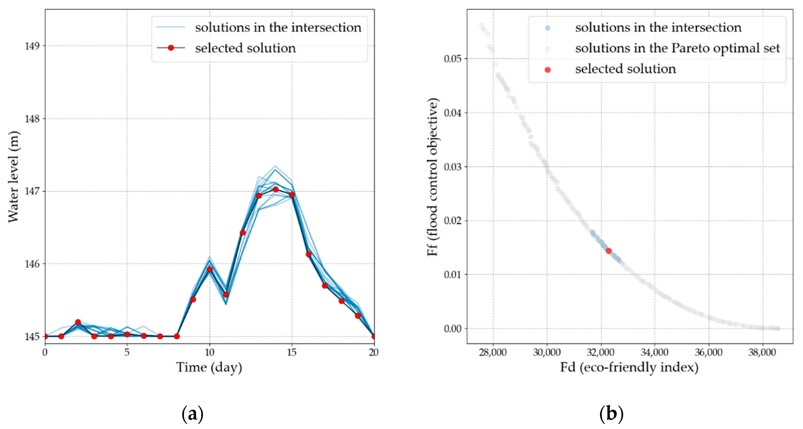
4.4. Solution Selection
5. Conclusions
Author Contributions
Funding
Institutional Review Board Statement
Informed Consent Statement
Data Availability Statement
Conflicts of Interest
Appendix A. Determination of the Ecological Flow Based on the Indicators of Hydrologic Alteration (IHA) Method

| Hydrologic Indicators of a High Pulse | Quantile | ||
|---|---|---|---|
| 75% | 50% | 25% | |
| Date of rise | 12 | 7 | 2 |
| Initial flow of the pulse (m3/s) | 23,500 | 21,150 | 20,250 |
| Duration of the high pulse (day) | 8 | 4 | 2 |
| No. of high pulses (times) | 2 | 1 | 1 |
| Peak flow of the high pulse (m3/s) | 30,800 | 25,450 | 21,200 |
| Rise rate (m3/s/d) | 2303 | 1932 | 1558 |
| Fall rate (m3/s/d) | −1105 | −1386 | −1766 |
| Rise duration (d) | 4 | 2 | 1 |
| Fall duration (d) | 4 | 2 | 1 |
| Index Number (Day) | 1 | 2 | 3 | 4 | 5 | 6 | 7 |
| Discharge (m3/s) | 14,800 | 14,900 | 14,800 | 15,500 | 15,100 | 14,700 | 15,100 |
| Index Number (Day) | 8 | 9 | 10 | 11 | 12 | 13 | 14 |
| Discharge (m3/s) | 15,400 | 15,000 | 18,483 | 21,966 | 25,450 | 23,666 | 21,883 |
| Index Number (Day) | 15 | 16 | 17 | 18 | 19 | 20 | 21 |
| Discharge (m3/s) | 20,100 | 19,500 | 22,000 | 21,800 | 22,200 | 23,200 | 25,200 |
References
- Yu, Y.; Wang, C.; Wang, P.; Hou, J.; Qian, J. Assessment of multi-objective reservoir operation in the middle and lower Yangtze River based on a flow regime influenced by the Three Gorges Project. Ecol. Inform. 2017, 38, 115–125. [Google Scholar] [CrossRef]
- Labadie, J.W. Optimal operation of multireservoir systems: State-of-the-art review. J. Water Resour. Plan. Manag. 2004, 130, 93–111. [Google Scholar] [CrossRef]
- Reddy, M.J.; Kumar, D.N. Optimal reservoir operation using multi-objective evolutionary algorithm. Water Resour. Manag. 2006, 20, 861–878. [Google Scholar] [CrossRef] [Green Version]
- Chou, F.N.F.; Wu, C.W. Stage-wise optimizing operating rules for flood control in a multi-purpose reservoir. J. Hydrol. 2015, 521, 245–260. [Google Scholar] [CrossRef]
- Dai, L.; Zhang, P.; Wang, Y.; Jiang, D.; Dai, H.; Mao, J.; Wang, M. Multi-objective optimization of cascade reservoirs using NSGA-II: A case study of the Three Gorges-Gezhouba cascade reservoirs in the middle Yangtze River, China. Hum. Ecol. Risk Assess. 2017, 23, 814–835. [Google Scholar] [CrossRef]
- Coello, C.A.C.; Lamont, G.B.; Van Veldhuizen, D.A.; Goldberg, D.E.; Koza, J.R. Evolutionary Algorithms for Solving Multi-Objective Problems; Springer: New York, NY, USA, 2007; ISBN 9780387310299. [Google Scholar]
- Van Veldhuizen, D.A.; Lamont, G.B. Multiobjective evolutionary algorithms: Analyzing the state-of-the-art. Evol. Comput. 2000, 8, 125–147. [Google Scholar] [CrossRef]
- Zhu, D.; Mei, Y.; Xu, X.; Chen, J.; Ben, Y. Optimal operation of complex flood control system composed of cascade reservoirs, navigation-power junctions, and flood storage areas. Water 2020, 12, 1883. [Google Scholar] [CrossRef]
- Zhou, A.; Qu, B.Y.; Li, H.; Zhao, S.Z.; Suganthan, P.N.; Zhangd, Q. Multiobjective evolutionary algorithms: A survey of the state of the art. Swarm Evol. Comput. 2011, 1, 32–49. [Google Scholar] [CrossRef]
- Deb, K. Multi-objective Optimisation Using Evolutionary Algorithms: An Introduction. In Multi-Objective Evolutionary Optimisation for Product Design and Manufacturing; Springer: London, UK, 2011. [Google Scholar]
- Reed, P.M.; Hadka, D.; Herman, J.D.; Kasprzyk, J.R.; Kollat, J.B. Evolutionary multiobjective optimization in water resources: The past, present, and future. Adv. Water Resour. 2013, 51, 438–456. [Google Scholar] [CrossRef] [Green Version]
- Adeyemo, J.A. Reservoir operation using multi-objective evolutionary algorithms—A review. Asian J. Sci. Res. 2011, 4, 16–27. [Google Scholar] [CrossRef]
- Chang, L.C.; Chang, F.J. Multi-objective evolutionary algorithm for operating parallel reservoir system. J. Hydrol. 2009, 377, 12–20. [Google Scholar] [CrossRef]
- Deb, K.; Pratap, A.; Agarwal, S.; Meyarivan, T. A fast and elitist multiobjective genetic algorithm: NSGA-II. IEEE Trans. Evol. Comput. 2002, 6, 182–197. [Google Scholar] [CrossRef] [Green Version]
- Qin, H.; Zhou, J.; Lu, Y.; Li, Y.; Zhang, Y. Multi-objective Cultured Differential Evolution for Generating Optimal Trade-offs in Reservoir Flood Control Operation. Water Resour. Manag. 2010, 24, 2611–2632. [Google Scholar] [CrossRef]
- Fotovatikhah, F.; Herrera, M.; Shamshirband, S.; Chau, K.W.; Ardabili, S.F.; Piran, M.J. Survey of computational intelligence as basis to big flood management: Challenges, research directions and future work. Eng. Appl. Comput. Fluid Mech. 2018, 12, 411–437. [Google Scholar] [CrossRef] [Green Version]
- Zhang, X.; Luo, J.; Sun, X.; Xie, J. Optimal reservoir flood operation using a decomposition-based multi-objective evolutionary algorithm. Eng. Optim. 2019, 51, 42–62. [Google Scholar] [CrossRef]
- Liu, D.; Huang, Q.; Yang, Y.; Liu, D.; Wei, X. Bi-objective algorithm based on NSGA-II framework to optimize reservoirs operation. J. Hydrol. 2020, 585, 124830. [Google Scholar] [CrossRef]
- Malekmohammadi, B.; Zahraie, B.; Kerachian, R. Ranking solutions of multi-objective reservoir operation optimization models using multi-criteria decision analysis. Expert Syst. Appl. 2011, 38, 7851–7863. [Google Scholar] [CrossRef]
- Tzeng, G.-H.; Huang, J.-J. Multiple Attribute Decision Making: Methods and Applications a State of the Art Survey; CRC Press: Boca Raton, FL, USA, 2011; ISBN 9781439861578. [Google Scholar]
- Kao, C. Weight determination for consistently ranking alternatives in multiple criteria decision analysis. Appl. Math. Model. 2010, 34, 1779–1787. [Google Scholar] [CrossRef]
- Jaini, N.; Utyuzhnikov, S. Trade-off ranking method for multi-criteria decision analysis. J. Multi-Criteria Decis. Anal. 2017, 24, 121–132. [Google Scholar] [CrossRef]
- Provost, F.; Fawcett, T. Data Science and its Relationship to Big Data and Data-Driven Decision Making. Big Data 2013, 1, 51–59. [Google Scholar] [CrossRef]
- Taboada, H.A.; Coit, D.W. Data mining techniques to facilitate the analysis of the pareto-optimal set for multiple objective problems. In Proceedings of the 2006 IIE Annual Conference and Exposition, Orlando, FL, USA, 20–24 May 2006. [Google Scholar]
- Suwal, N.; Huang, X.; Kuriqi, A.; Chen, Y.; Pandey, K.P.; Bhattarai, K.P. Optimisation of cascade reservoir operation considering environmental flows for different environmental management classes. Renew. Energy 2020, 158, 453–464. [Google Scholar] [CrossRef]
- Dumedah, G.; Berg, A.A.; Wineberg, M.; Collier, R. Selecting Model Parameter Sets from a Trade-off Surface Generated from the Non-Dominated Sorting Genetic Algorithm-II. Water Resour. Manag. 2010, 24, 4469–4489. [Google Scholar] [CrossRef]
- Sato, Y.; Izui, K.; Yamada, T.; Nishiwaki, S. Data mining based on clustering and association rule analysis for knowledge discovery in multiobjective topology optimization. Expert Syst. Appl. 2019, 119, 247–261. [Google Scholar] [CrossRef]
- Liao, T.W. Clustering of time series data—A survey. Pattern Recognit. 2005, 38, 1857–1874. [Google Scholar] [CrossRef]
- Xu, D.; Tian, Y. A Comprehensive Survey of Clustering Algorithms. Ann. Data Sci. 2015, 2, 165–193. [Google Scholar] [CrossRef] [Green Version]
- Wang, X.; Mei, Y.; Cai, H.; Cong, X. A new fluctuation index: Characteristics and application to hydro-wind systems. Energies 2016, 9, 114. [Google Scholar] [CrossRef] [Green Version]
- Rodriguez, A.; Laio, A. Clustering by fast search and find of density peaks. Science 2014, 344, 1492–1496. [Google Scholar] [CrossRef] [PubMed] [Green Version]
- Liu, R.; Wang, H.; Yu, X. Shared-nearest-neighbor-based clustering by fast search and find of density peaks. Inf. Sci. 2018, 450, 200–226. [Google Scholar] [CrossRef]
- Zhang, Y.; Zhou, J.; Li, C.; Chen, F. Integrated utilization of the Three Gorges Cascade for navigation and power generation in flood season. Shuili Xuebao 2017, 48, 31–40. [Google Scholar] [CrossRef]
- Ban, X.; Diplas, P.; Shih, W.R.; Pan, B.; Xiao, F.; Yun, D. Impact of Three Gorges Dam operation on the spawning success of four major Chinese carps. Ecol. Eng. 2019. [Google Scholar] [CrossRef]
- Tsai, W.P.; Chang, F.J.; Chang, L.C.; Herricks, E.E. AI techniques for optimizing multi-objective reservoir operation upon human and riverine ecosystem demands. J. Hydrol. 2015, 530, 634–644. [Google Scholar] [CrossRef]
- Ameur, M.; Kharbouch, Y.; Mimet, A. Optimization of passive design features for a naturally ventilated residential building according to the bioclimatic architecture concept and considering the northern Morocco climate. Build. Simul. 2020, 13, 677–689. [Google Scholar] [CrossRef]
- Marler, R.T.; Arora, J.S. Survey of multi-objective optimization methods for engineering. Struct. Multidiscip. Optim. 2004, 26, 369–395. [Google Scholar] [CrossRef]
- Jain, A.K. Data clustering: 50 years beyond K-means. Pattern Recognit. Lett. 2010, 31, 651–666. [Google Scholar] [CrossRef]
- Gentle, J.E.; Kaufman, L.; Rousseuw, P.J. Finding Groups in Data: An Introduction to Cluster Analysis. Biometrics 1991, 47, 788. [Google Scholar] [CrossRef]
- Caliński, T.; Harabasz, J. A dendrite method for cluster analysis. Commun. Stat. 1974, 3, 1–27. [Google Scholar]
- Taboada, H.A.; Baheranwala, F.; Coit, D.W.; Wattanapongsakorn, N. Practical solutions for multi-objective optimization: An application to system reliability design problems. Reliab. Eng. Syst. Saf. 2007, 92, 314–322. [Google Scholar] [CrossRef]
- Satopää, V.; Albrecht, J.; Irwin, D.; Raghavan, B. Finding a “kneedle” in a haystack: Detecting knee points in system behavior. Proc. Int. Conf. Distrib. Comput. Syst. 2011, 166–171. [Google Scholar] [CrossRef] [Green Version]
- Berndt, D.; Clifford, J. Using dynamic time warping to find patterns in time series. Knowl. Discov. Databases Workshop 1994, 398, 359–370. [Google Scholar]
- Yuan, G.; Sun, P.; Zhao, J.; Li, D.; Wang, C. A review of moving object trajectory clustering algorithms. Artif. Intell. Rev. 2017, 47, 123–144. [Google Scholar] [CrossRef]
- Rousseeuw, P.J. Silhouettes: A graphical aid to the interpretation and validation of cluster analysis. J. Comput. Appl. Math. 1987, 20, 53–65. [Google Scholar] [CrossRef] [Green Version]
- Arbelaitz, O.; Gurrutxaga, I.; Muguerza, J.; Pérez, J.M.; Perona, I. An extensive comparative study of cluster validity indices. Pattern Recognit. 2013, 46, 243–256. [Google Scholar] [CrossRef]
- Aghabozorgi, S.; Shirkhorshidi, A.S.; Ying Wah, T. Time-series clustering—A decade review. Inf. Syst. 2015, 53, 16–38. [Google Scholar] [CrossRef]
- Ruiz, L.G.B.; Pegalajar, M.C.; Arcucci, R.; Molina-Solana, M. A time-series clustering methodology for knowledge extraction in energy consumption data. Expert Syst. Appl. 2020, 160, 113731. [Google Scholar] [CrossRef]
- Wang, H.; Brill, E.D.; Ranjithan, R.S.; Sankarasubramanian, A. A framework for incorporating ecological releases in single reservoir operation. Adv. Water Resour. 2015, 78, 9–21. [Google Scholar] [CrossRef]
- Mathews, R.; Richter, B.D. Application of the indicators of hydrologic alteration software in environmental flow setting. J. Am. Water Resour. Assoc. 2007, 43, 1400–1413. [Google Scholar] [CrossRef]


| Description | DTW-DPC | ED-DPC | MWFSM-DPC | |
|---|---|---|---|---|
| No. of clusters in decision space | 5 | 5 | 7 | |
| Sil | 0.503 | 0.429 | 0.346 | |
| No. of solutions in the cluster | cluster 1 | 53 | 40 | 14 |
| cluster 2 | 46 | 97 | 9 | |
| cluster 3 | 36 | 28 | 16 | |
| cluster 4 | 40 | 15 | 36 | |
| cluster 5 | 25 | 20 | 71 | |
| cluster 6 | 20 | |||
| cluster 7 | 34 | |||
| Pareto Cluster | Cluster 1 | Cluster 2 | Cluster 3 | Cluster 4 | Cluster 5 |
| No. of solutions in the intersection | 0 | 9 | 0 | 19 | 0 |
| Pareto Cluster | Cluster 6 | Cluster 7 | Cluster 8 | Cluster 9 | Cluster 10 |
| No. of solutions in the intersection | 2 | 22 | 0 | 0 | 19 |
Publisher’s Note: MDPI stays neutral with regard to jurisdictional claims in published maps and institutional affiliations. |
© 2021 by the authors. Licensee MDPI, Basel, Switzerland. This article is an open access article distributed under the terms and conditions of the Creative Commons Attribution (CC BY) license (https://creativecommons.org/licenses/by/4.0/).
Share and Cite
Kong, Y.; Mei, Y.; Wang, X.; Ben, Y. Solution Selection from a Pareto Optimal Set of Multi-Objective Reservoir Operation via Clustering Operation Processes and Objective Values. Water 2021, 13, 1046. https://0-doi-org.brum.beds.ac.uk/10.3390/w13081046
Kong Y, Mei Y, Wang X, Ben Y. Solution Selection from a Pareto Optimal Set of Multi-Objective Reservoir Operation via Clustering Operation Processes and Objective Values. Water. 2021; 13(8):1046. https://0-doi-org.brum.beds.ac.uk/10.3390/w13081046
Chicago/Turabian StyleKong, Yanjun, Yadong Mei, Xianxun Wang, and Yue Ben. 2021. "Solution Selection from a Pareto Optimal Set of Multi-Objective Reservoir Operation via Clustering Operation Processes and Objective Values" Water 13, no. 8: 1046. https://0-doi-org.brum.beds.ac.uk/10.3390/w13081046