Article

Roadmap for Determining Natural Background Levels of Trace Metals in Groundwater

1
Geological Survey of Denmark and Greenland (GEUS), C.F. Møllers Allé 8, 8000 Aarhus C, Denmark
2
Geological Survey of Denmark and Greenland (GEUS), Øster Voldgade 10, 1350 København K, Denmark
3
Department of Public Health, Research Unit for Environment, Work and Health, Aarhus University, Bartholins Allé 2, 8000 Aarhus C, Denmark
*
Author to whom correspondence should be addressed.
Submission received: 3 March 2021 / Revised: 25 April 2021 / Accepted: 28 April 2021 / Published: 30 April 2021
(This article belongs to the Special Issue Natural Background Levels in Groundwater)

Abstract

:
Determining natural background levels (NBLs) is a fundamental step in assessing the chemical status of groundwater bodies in the EU, as stipulated by the Water Framework and Groundwater Directives. The major challenges in deriving NBLs for trace metals are understanding the interaction of natural and anthropogenic processes and identifying the boundary between pristine and polluted groundwater. Thus, the purpose of this paper is to present a roadmap guiding the process of method selection for setting meaningful NBLs of trace metals in groundwater. To develop the roadmap, we compared and critically assessed how three methods for excluding polluted sampling points affect the NBLs for As, Cd, Cr, Cu, Ni, and Zn in Danish aquifers. These methods exclude sampling points based on (1) the primary use of the well (or sampling purpose), (2) the dominating anthropogenic pressure in the vicinity of the well, or (3) a combination of pollution indicators (NO3, pesticides, organic micropollutants). Except for Ni, the NBLs derived from the three methods did not differ significantly, indicating that the data pre-selection based on the primary use of the wells is an important step in assuring the removal of anthropogenically influenced points. However, this pre-selection could limit the data representativity with respect to the different groundwater types. The roadmap (a step-by-step guideline) can be used at the national scale in countries with varying data availability.

1. Introduction

Trace metals are ubiquitous in groundwater in concentrations that are determined primarily by natural processes, but in addition, they may be affected by anthropogenic factors. Significant exceedances of the natural backgrounds are a question of anthropogenic pollution or other human activities changing the natural geochemistry that may eventually require the development of action plans and remediation measures. Therefore, the assessment of natural background levels (NBLs) for trace metals is a prerequisite to determine whether observed concentrations are affected by human activities. In that case, remediation measures need to be introduced to protect the legitimate groundwater uses and groundwater-dependent terrestrial and associated aquatic ecosystems. The remediation measures then aim at reducing the groundwater concentrations below a specific threshold value (TV) for the pollutant, defined by the member states based on the estimated NBL for the pollutant according to EU legislation and guidance [1,2,3].

1.1. Derivation of NBLs and TVs for Assessment of Groundwater Chemical Status in EU

The European Water Framework Directive (WFD) [1] and Groundwater Directive (GWD) [2] stipulate that groundwater status must be assessed by the member states and that good status must be achieved to protect human health and groundwater-dependent or associated ecosystems, e.g., wetlands, and transitional and coastal waters. According to the GWD, TVs are groundwater quality standards for pollutants or groups of pollutants established by the individual member states for ensuring compliance with the definition of good chemical status of groundwater bodies. The WFD defines a groundwater body as a distinct volume of groundwater within an aquifer or system of aquifers. “Aquifer” is then defined as “a subsurface layer or layers of rock or other geological strata of sufficient porosity and permeability to allow either a significant flow of groundwater or the abstraction of significant quantities of groundwater” [1]. The national authorities of the member states derive these TVs as the basis for the groundwater status assessments. Annex II.A of GWD (see Appendix A for direct quote) provides a general guideline on the TV derivation, while more details can be found in Guidance Document No. 18 [3]. Hinsby et al., 2008 [4] presented a selection of application examples.
The groundwater chemical status provisions of the GWD only apply for anthropogenically altered conditions. Thus, a fundamental first step in establishing TVs is assessing the NBLs, i.e., the naturally occurring concentrations of substances for different hydrogeological conditions. The definition provided in the GWD (Article 2.5) states that “…’background level’ means the concentration of a substance or the value of an indicator in a body of groundwater corresponding to no, or only very minor, anthropogenic alterations to undisturbed conditions”. Member States are free to apply their own approach for identifying these NBLs, depending on existing studies and conceptual models of the groundwater bodies [3]. According to the widely used BRIDGE methodology [4], NBLs are derived as the 90th (or 97th) percentiles of a pre-selected dataset, which should approximate a natural groundwater composition of a given aquifer type [4] (see details in Section 3.2). The 90th percentile was suggested for small datasets (<~60 sampling points) or datasets where human impact cannot be excluded, while the 97th percentile is for groundwater bodies where all data points represent groundwater with a natural composition [4]. Guidance Document No. 18 [3] also refers to the BRIDGE methodology and mentions the 90th percentile as a practical criterion for setting the NBLs.
The NBL derivation in this context is similar to determining groundwater baseline quality with statistical methods, which aim at distinguishing anomalies from typical values [5]. Even though sometimes NBL and baseline quality are used as synonyms, there is an important distinction to be made. Groundwater baseline quality is “the range of concentrations derived entirely from natural, geological, biological or atmospheric sources, under conditions not perturbed by anthropogenic activity” [5], while the NBLs could include minor anthropogenic influences (see definition above) and is represented by a single value from which TV can be derived. Identifying groundwater baseline properties could rely on various other approaches (next to the purely statistical ones), e.g., use of historical data (pre-industrial conditions), down-gradient profiles, extrapolation from adjacent areas with similar geology, groundwater dating, and geochemical modeling [5]. Determining the groundwater baseline quality is beyond the scope of this study, where we focus on NBLs.

1.2. Purpose of This Study

The major challenges in deriving NBLs are (1) understanding how the interaction of natural and anthropogenic processes affects groundwater quality and (2) identifying the boundary between pristine (or nearly pristine) and polluted groundwater. EU member states need to set NBLs to be able to define TVs for the chemical status assessment of groundwater bodies, stipulated in the EU legislation. It was previously demonstrated that a very wide range of TVs is derived and reported by the member states, partly because of the NBLs derivation, and that further harmonization is warranted [6,7]. Therefore, the general objective of this study is to present a roadmap—a guideline on how to derive meaningful NBLs for trace metals, which can be an especially challenging task in the context of intensive and widespread agriculture, and extensive groundwater pumping for drinking water supply in urban areas. Our specific objectives are:
(1)
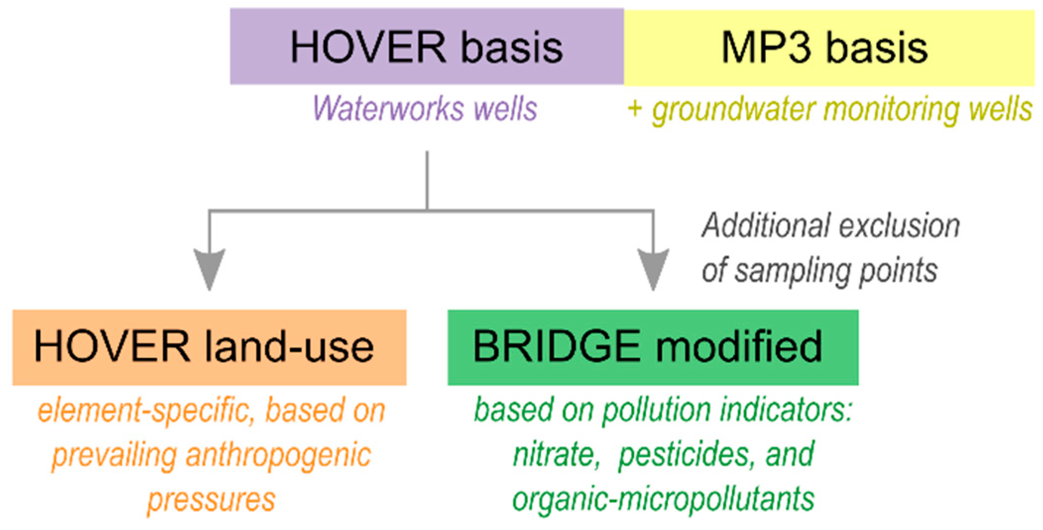
To apply and compare three different methods for excluding anthropogenically influenced points when calculating the NBLs for trace metals in Denmark. These methods rely on the exclusion of water sampling points from the datasets, based on:
  • Primary use of the well (and/or the sampling purpose);
  • Dominating land-use (thus, potential anthropogenic pressure);
  • Combination of pollution indicators.
(2)
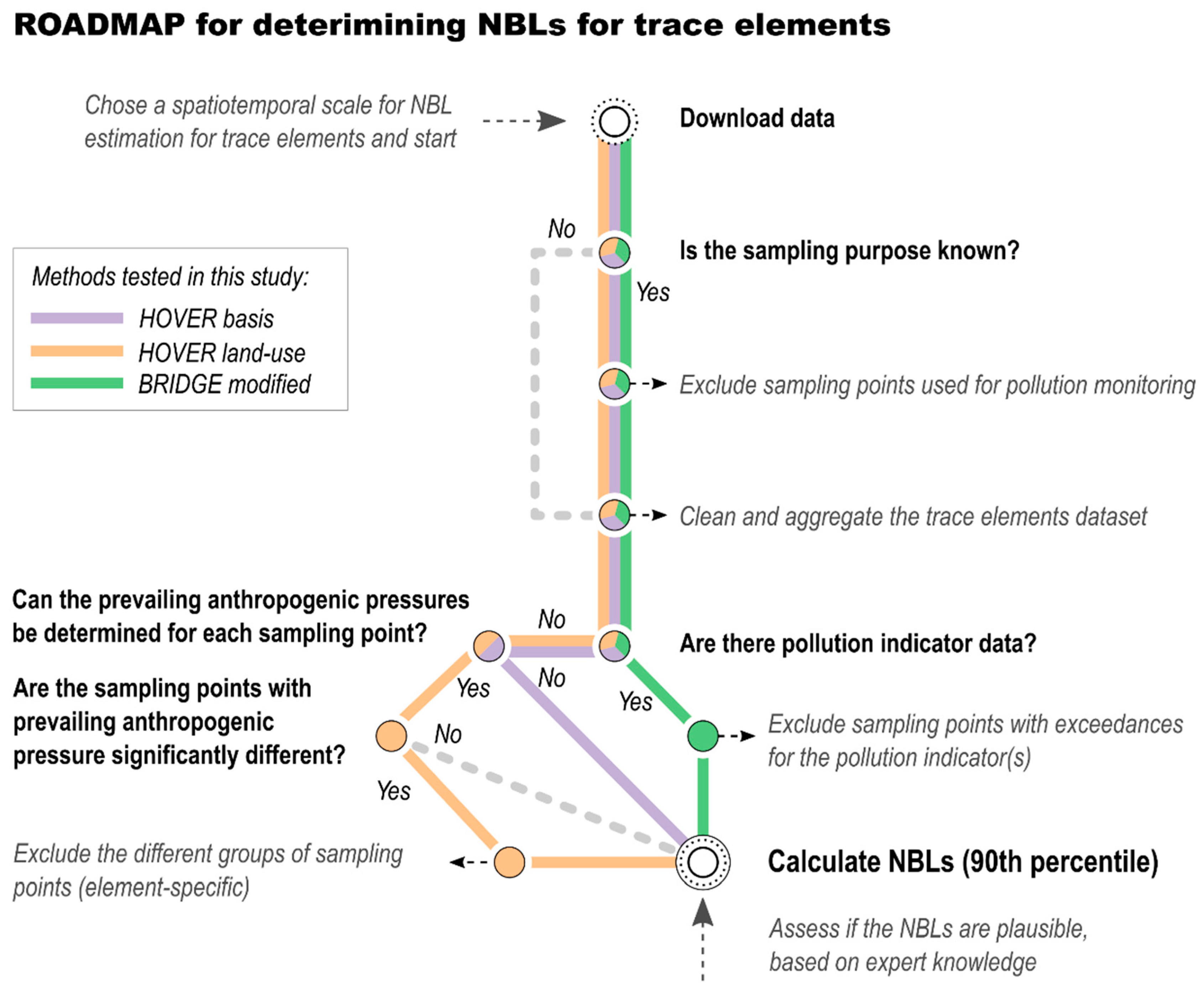
To critically assess, i.e., discuss requirements, advantages, and disadvantages of the individual methods, and on that basis to develop a universally applicable roadmap for NBLs derivation at the national scale.
Through this process, we aim to demonstrate also how combining several methods, using several types of data may compensate for the individual limitations of the methods.

2. Study Setting

2.1. Denmark—A Case Study with Widespread and Intensive Agricultural Pressure

Denmark is an EU country with an area of ~43,000 km2 and a population of ~5.8 million (2018, Eurostat). Agricultural land covers 61% of Denmark (Figure 1a), a major part of which is used for the annual cultivation of grains, grass in crop rotation, and rapeseed. Forests cover 13%, other nature (wet or dry, incl. meadows and heaths) 9%, and the buildings and built-up areas cover 7% (the land-cover statistics isfrom Statistic Denmark https://www.dst.dk (accessed on 15 October 2020)). This places Denmark in third place in Europe, after Ireland and U.K., on percent used agricultural area, according to Eurostat (see Farms and farmland statistics, https://ec.europa.eu/eurostat/statistics-explained/ (accessed on 1 January 2020)). In 2019, there were about 33,600 farms with a total number of 1.49 million cattle and 12.3 million pigs. Denmark also has a very high production number of intensively reared pigs (>30 million/year) [8] and relatively high cow milk production (5693 million kg for 2019). About 11% of the agricultural land was either cultivated organically or is being converted to organic farming in 2019.
The Danish landscape was shaped by a sequence of Pleistocene glaciations and postglacial processes, and the resulting topography is flat to gently undulating with a maximum elevation of 170 m [9].
The drinking water supply in Denmark is highly decentralized (~2600 active public waterworks) and relies 100% on groundwater. The groundwater for drinking water purposes is extracted from aquifers primarily composed of: (1) Quaternary glacio-fluvial sand and gravel deposits, (2) Upper Cretaceous and Danian limestone and chalk, and (3) Miocene quartz sand and micaceous sand [10]. The island of Bornholm is an exception, as there are various older fractured aquifers (see Figure S1). A brief introduction to the Quaternary and pre-Quaternary geology [10,11] of Denmark is provided in Supplementary Materials.
Based on the National Water Resources Model for Denmark, DK model (https://vandmodel.dk/ (accessed on 29 April 2021)), 2050 groundwater bodies have been delineated in Denmark [12]. The WFD definition of groundwater body (see Section 1.1) was followed, and the specific delineation criteria included [12]: (1) a minimum thickness of 2 m and minimum extend of 25 ha, (2) aquifers of the same geological type were grouped together only if there was a hydraulic contact between them (existing low-permeability layers were <2 m thick). In some cases, large groundwater bodies (>100 ha) were subdivided based on their hydrological and geomorphological characteristics, or differences in aquifer thickness, to limit the heterogeneity within the groundwater bodies. The majority of the 2050 Danish groundwater bodies do not have any water analyses. In this study, we investigated analyses of trace metals from drinking water wells, tapping into 451 of them (Figure 1b). Because the 451 groundwater bodies have varying area and volume (and data availability), for the purposes of deriving NBLs here, we grouped them according to four main aquifer types: (1) Quaternary sand, (2) Carbonate fractured rocks, (3) pre-Quaternary sand, and (4) the diverse geological units on the island of Bornholm (Figure 1b).

2.2. TV and NBL Assessments in Denmark

The national TVs for trace metals in Denmark originate from the national drinking water legislation, which agrees with the EU Drinking Water Directive [13]. In accordance with Guidance Document No. 18 [3], higher TVs are established for Danish groundwater bodies, where the NBLs exceed the national TVs. The national TVs could also be lowered if the drinking water standards do not provide sufficient protection of groundwater-dependent terrestrial or associated aquatic ecosystems [4], but this approach has not yet been applied in Denmark. Table 1 shows the current national groundwater TVs, set by the Danish Environmental Protection Agency (Danish EPA), and the Danish drinking water standards (BEK nr 1070 af 28/10/2019).
NBLs for trace metals have been derived in Denmark as part of the chemical status assessment of Danish groundwater bodies in the second and the ongoing third River Basin Management Plans, abbreviated further as MP2 (period 2015–2021) and MP3 (2021–2027); and as part of the research projects BRIDGE and HOVER. BRIDGE is an acronym for the project “Background criteria for the identification of groundwater thresholds”, which ran in the period January 2005–December 2006 (https://cordis.europa.eu/project/id/6538 (accessed on 29 April 2021)) and HOVER is an acronym of the ongoing project “Hydrogeological processes and Geological settings over Europe controlling dissolved geogenic and anthropogenic elements in groundwater of relevance to human health and the status of dependent ecosystems” in the GeoERA program (https://geoera.eu/ (accessed on 29 April 2021)).
In MP2, NBLs for As and Ni were derived as the 90th percentile of the mean concentrations at the sampling points for 2007–2013, or if not available, for 2000–2006 (see Supplementary Materials for more details).
The national NBLs for trace elements (Al, As, Pb, Cd, Hg, Ni, Pb, Cu, Cr, and Zn) is currently under revision for the MP3. This time, a larger focus is placed on the different hydrogeochemical conditions in Danish aquifers. Groundwater types are distinguished based on the redox, pH, and organic matter content (as non-volatile organic carbon, NVOC) [14]. Other differences from MP2 include aquifer type classification simplification and a different sampling period (2000–2018). NBLs were derived as the 90th percentile of the mean concentration calculated from the annual means in the period at pre-selected sampling points. Expert assessment deemed some of the calculated NBLs unreliable due to potential anthropogenic influences [14]. For example, the NBL for Ni in some aquifers were not used due to known elevated concentrations caused by oxidation and reduction of iron sulfides and manganese oxides, respectively, because of (1) initial lowering of the water table due to excessive abstraction and the oxidation of nickel containing pyrite followed by (2) rising water tables that submerge and reduce manganese oxides releasing adsorbed nickel [15,16,17].
BRIDGE project developed a tiered methodology for TV derivation [4]. The Danish case study focused on the TVs for N and P based on environmental objectives for dependent ecosystems at the Odense river basin, located on the isle of Fyn (Figure 1). Additionally, NBLs for other elements, including As, were calculated based on pre-selection criteria. A summary of these criteria commonly referred to in the NBL literature as the “BRIDGE method” is presented in SM.
A task in the ongoing HOVER project aims at proposing a common methodology to identify the main geological factors and hydrogeological processes controlling the distribution of NBLs of selected dissolved elements [18]. The tested method included identifying anthropogenic pressures and relating those to specific dissolved solutes (As, Cd, Cr, Cu, Ni, Zn, F, Cl, SO4) in areas under agricultural, industrial, mining, and urban influences. A variety of applications are presented for different settings in Europe in [18].

3. Materials and Methods

3.1. Identifying Anthropogenically Influenced Water Sampling Points

To develop a road map for determining NBLs for trace metals, we apply, compare, and critically assess three methods for identifying and excluding anthropogenically influenced groundwater sampling points: (1) the basis level method relying on a pre-selection of sampling points only, (2) a land-use based method developed in HOVER [18], and (3) a modification of the BRIDGE method (Figure 2).
The basis level method relies on a pre-selection of wells based on their primary usage. The chemical analyses of groundwater samples from these pre-selected wells form the dataset used further. Two versions of this method are compared to each other to assess the effect of both sampling pre-selection and different data handling. The HOVER basis version includes only waterworks wells used for drinking water production. While for MP3 basis version (the official national NBL derivation part of MP3), wells of the national groundwater monitoring program are also included [14]. Even though such pre-selection is possible, there could still be sampling points influenced by anthropogenic activities. Thus, to further “clean” the dataset, we tested HOVER land-use and BRIDGE modified methods.
HOVER land-use method [18] relies on a land-use-based approach for identifying anthropogenic pressures and excluding sampling points potentially influenced by it. The dominating anthropogenic pressure for each sampling point was established based on the areal proportion of the land-use types in the vicinity of the well. For each heavy metal, the groups of sampling points with different anthropogenic pressure were compared, and the significantly different groups were excluded. The group comparison was performed based on Kruskal–Wallis test with a post-hoc Nemenyi test, and the statistical significance was assessed at the 95% confidence level [18]. The statistical testing is performed for each element separately, so different groundwater sampling points are excluded for different elements.
BRIDGE modified relies on a combination of pollution indicators, including NO3, pesticides, and organic micropollutants. Nitrate and pesticides are used here as indicators for agricultural pollution, while the organic micropollutants serve as indicators for urban or industrial pollution. We consider a water sampling point to be polluted and exclude it from the dataset if at least one of the following conditions is true:
  • NO3 > 10 mg/L—a condition from the original BRIDGE method [4];
  • At least one of the analyzed pesticides (metabolites, degradation, or transformation products) is exceeding the drinking water standard for individual pesticides (0.1 µg/L) or the sum of the quantified pesticides (0.5 µg/L);
  • At least one of the organic micropollutants is exceeding the specific drinking water standards.
The HOVER basis dataset is used as a starting point for applying both the HOVER land-use and BRIDGE modified. Thus, when comparing the NBLs derived from the HOVER land-use and BRIDGE modified to those derived based on HOVER basis, we assess the effect of additional removal of potentially polluted sampling points. The assumption underlying our assessment is that this removal should result in lowered NBLs for the selected trace metals.

3.2. Trace Metals—Sources and Geochemical Controls

The main geogenic and anthropogenic sources and the relevant geochemical controls of the selected trace metals (As, Cd, Cr, Cu, Ni, and Zn) are summarized in Table A1 [5,19]. The main geochemical processes governing their concentrations in groundwater are dissolution of minerals or desorption from either Fe and Mn (oxy)hydroxides, clays, calcite surfaces, or organic matter (Table A1). Both industrial and urban areas may be sources of potential anthropogenic pollution, but intensive agriculture could also be a major contributor, as some of these elements are present in either pesticides or fertilizers (Table A1). The mobility of these elements in groundwater is directly or indirectly controlled by pH and redox conditions (Table A1); therefore, the groundwater pH and redox state at the sampling point should also be considered when calculating the NBLs for these elements.
We classified the sampling points into the following pH classes [18]:
  • Acidic (pH < 7);
  • Basic (pH > 7.5);
  • Neutral (7 ≤ pH ≤ 7.5).
For the redox classification, we used an algorithm based on the O2, NO3 and Fe content [16]. The algorithm conditions are given in the brackets (more details in [16]):
  • Oxic (A type, if NO3 > 1 mg/L and Fe < 0.2 mg/L and O2 ≥ 1 mg/L);
  • Anoxic, nitrate reducing (B type, if NO3 > 1 mg/L and Fe < 0.2 mg/L and O2 < 1 mg/L);
  • Reduced (C and D types, if NO3 ≤ 1 mg/L and Fe ≥ 0.2 mg/L);
  • Mixed (X and Y types, do not fulfil the conditions for A, B, C, and D types).

3.3. Data Sources and Processing

All chemical data originate from the open and freely accessible national well database Jupiter, hosted by the Geological Survey of Denmark and Greenland (GEUS). Groundwater sampling follows the procedures outlined in the national guidelines (e.g., https://www.geus.dk/media/8324/g02_proevetagning-okt12_uk.pdf (accessed on 29 April 2021)). Dataset-specific details are provided below.

3.3.1. Primary Chemical Dataset (HOVER Basis)

The raw chemical data are from the Danish groundwater monitoring program dataset extracted in July 2019 [20]. The general quality assurance is reported in [20], and the project-specific data pre-treatment is detailed in [18]. In brief, the data pre-treatment included various element-specific quality checks, treatment of all values below the limit of detection, and aggregation on sampling point level. The sampling points were limited to the waterworks wells used for the drinking water supply in Denmark. This differs from the MP3 basis dataset, in which also the groundwater monitoring wells were included. The other methodological differences in the data preparation for MP3 basis and HOVER basis methods are summarized in Table 2.

3.3.2. Complementary Data

The data necessary for classifying all water sampling points according to geology, pH, and redox types is also from [20]. The geology classification is derived from the established link between groundwater bodies and sampling points [12]. All sampling points included in this study were linked to a specific groundwater body (n = 451, Figure 1b); thus, it was possible to classify them in one of the main aquifer types (Figure S2). The same NO3 data was used also for BRIDGE modified.
To apply HOVER land-use, we used Corine land cover (CLC-12) for Denmark (v.1 from October 2014 in 1: 100,000 scale with reference year 2012; https://download.kortforsyningen.dk/content/corine-land-cover (accessed on 20 May 2020)) (Figure 1a). A buffer of 1 km around each sampling point was used to determine the areal proportion of the different land-cover types. This approximates the catchment area of individual wells, as these are unknown at the national scale. Most likely, the actual catchment areas are not circular and differ in size. The prevailing anthropogenic pressure based on the dominating type (i.e., the type with the largest areal proportion within the 1 km buffer) includes:
  • Urban—continuous and discontinuous urban fabric (CLC-12, Level 2 “urban fabric”);
  • Industrial—industrial or commercial units, road and rail networks, and associated land, port areas, and airports (CLC-12, Level 2 “industrial, commercial and transport units”);
  • Agricultural—non-irrigated arable land, fruit trees, and berry plantation, pastures, complex cultivation patterns, land principally occupied by agriculture with significant areas of natural vegetation (CLC-12, Level 1 “agricultural areas”);
  • Mining—mineral extraction sites, dump sites, and construction sites (CLC-12, Level 2 “mine, dump, and construction sites”).
A sampling point was assigned the value “natural or other” if none of the listed above were dominating in 1 km buffer area, i.e., the dominating land-use type belonged to “forests and semi-natural areas”, “wetlands”, or “water bodies” (CLC-12 Level 1).
To apply BRIDGE modified, we also used two other aggregated datasets that were originally prepared (extracted, quality checked, cleaned, and aggregated) for the purposes of MP3. The first one contained data for five pesticides of interest: DEIA (desethyl-desisopropyl-atrazine, a degradation product of atrazine), BAM (2,6-dichlorbenzamide, a degradation product of dichlobenil and chlorthiamid), triazole, DPC (desphenyl chloridazon, a degradation product of chloridazon), and DMS (N,N-dimethylsulfamide, a degradation product of tolylfluanid and dichlofluanid); and, the maximum concentration of all analyzed pesticides and the sum of the pesticides for all sampling points with at least one pesticide analysis in the period 2013–2019. “Pesticide” term here also includes the metabolites, degradation, and transformation products of the pesticides. The aggregation on a sampling point for all MP3 projects was based on the mean calculated from the annual mean concentrations (2013–2019). This data was available for 12,688 sampling points, so we could classify almost all sampling points of the BRIDGE basis dataset (n = 6221, 97.4%) into (a) complying with, or (b) exceeding the drinking water quality criteria (0.1 µg/L for individual pesticides, 0.5 µg/L for the sum of pesticides). If there was exceedance for at least one of the parameters, then the water sampling point was assumed to be influenced by anthropogenic pollution.
The second aggregated dataset contained data for 50 different chemical compounds belonging to the groups’ chlorinated solvents and degradation products, water-soluble solvents, phenolic compounds, MTBE (methyl tert-butyl ether), BTEXN (benzene, toluene, ethylbenzene, xylenes, and naphthalene) compounds, PFAS (per- and polyfluoroalkyl substances), cyanides, as well as the sum of PFAS and sum of chlorinated solvents and degradation products. Although there were data for 15,235 sampling points, only 48.2% (n = 3079) of the sampling points included in the HOVER basis dataset were covered. We classified these sampling points into (a) complying with or (b) exceeding the specific national standards set by the Danish EPA. If there was exceedance for at least one of the parameters, then the water sampling point was assumed to be influenced by anthropogenic pollution.
Additionally, we discuss the potential and limitations of applying other methods. We also use Cl and Na data [20] as in the original BRIDGE method [4]. Cl and SO4 trends [21] were discussed as indicators for overexploitation of groundwater; and, the groundwater age based on tritium and chlorofluorocarbon CFC (11, 12, 113) [20] was discussed as an indicator for pre-industrial groundwater quality and pollution vulnerability.

3.4. Statistics and Software

TVs, and, respectively, NBLs, can be established at the national, river basin district, or at the level of the groundwater body, or groups of groundwater bodies [2]. Here we calculate the NBLs as the 90th percentile for aquifer types (i.e., groups of groundwater bodies of the same type). The 90th percentile is calculated with R package stats v.4.0.2 [22] (“quantile” function, type 7 [23]). A two-sided nonparametric confidence interval (CI) for the 90th percentile at the 95% confidence level was calculated with R package EnvStats v. 2.4.0 [24] (“eqnpar” function). CI could not be calculated for sub-sets with less than 30 sampling points; thus, we only report NBLs and their 95% CI for the classes with 30 or more sampling points. We construe no difference between the NBLs calculated based on the different methods if there is an overlap between the 95% CI (visualized as error bars). The distributions of heavy metal concentrations are presented graphically with empirical cumulative distribution plots. All calculations and graphs are completed in R v.4.0.2 [22] with the additional R packages: stringr v. 1.4.0 [25], ggplot2 v. 3.3.2 [26], tidyr v. 1.1.2 [27], dplyr v. 1.0.2 [28], and data.table v. 1.13.0 [29]. All maps were prepared in QGIS [30], and the roadmap was created in Inkscape [31].

4. Results

4.1. Trace Metals in Danish Groundwater Used for Drinking Water Purposes

The concentration distribution for trace metals in Danish groundwater used for drinking water production, based on the HOVER basis dataset, is shown in Figure 3. The concentration levels on a national scale rank in the order from low to high: Cd < Cr < Cu < Ni < As < Zn. Figure 4 shows the spatial distribution of sampling points exceeding the national TVs for As and Ni (Table 1) for the main aquifer types. The rest of the trace metals do not exceed the TVs and have sparse spatial coverage, so they are not shown.

4.2. Dataset Representativity

The percent sampling points in the HOVER basis dataset falling in different aquifer types, pH and redox classes, and prevailing anthropogenic pressure are presented in Table A2. The dataset is biased toward Quaternary sand aquifers (53–64%) with neutral pH (53–57%), reduced conditions (76–83%), and agricultural pressures (75–86%) (Table A2). The bias toward agriculturally dominated locations is because of the high percentage of arable land in Denmark (61%). The waterworks wells are usually located in areas with only minor point-source pollution, as the Danish drinking water supply relies on clean groundwater, which is treated only with conventional systems (aeration and sand-filtration). Thus, the low number of points with dominating industrial, mining, or urban influences could be explained by the pre-selection of sampling points, which here include only the waterworks wells.
There is an incomplete data coverage for pH, where 10–14% of the sampling points with trace metal data had no reported pH in the period (2009–2018). For redox, this percentage was <1%. The spatial distribution by pH and redox is shown in Figure 5. Empirical cumulative distribution plots stratified by aquifer, pH, redox, and prevailing anthropogenic pressure type can be seen in Figures S3–S6.

4.3. Excluding Sampling Points Due to Anthropogenic Influences

There was no additional assessment of pressures and exclusion of potentially polluted sampling points for the HOVER basis (and MP3 basis) method prior to NBL calculation. However, many sampling points were initially excluded as they did not belong to waterworks wells (or groundwater monitoring wells for MP3 basis). For example, polluted wells (e.g., decommissioned due to pollution), those for monitoring of polluted sites (point-source monitoring), and the remediation wells were excluded. To put this into context, the cleaned and aggregated trace elements dataset for the status assessment of the Danish groundwater bodies (part of MP3, sampling period 2013–2019) included 9343 sampling points belonging to (1) waterworks wells used for drinking water purposes (71.1%), (2) point-source pollution monitoring wells (6.3%), (3) wells part of the national groundwater monitoring or mapping program (21.6%), and (4) wells serving other purposes (1.1%). Thus, we could conclude that the pre-selection used in HOVER basis excluded about one-third of the sampling points with reliable data for trace metals in Denmark. Even though such pre-selection is made, it is possible that some of the sampling points in the HOVER basis dataset are influenced by anthropogenic activities. To further “clean” the dataset, we tested the HOVER land-use and BRIDGE modified methods.
Before calculating the NBLs for HOVER land-use, we excluded all sampling points with both industrial and urban prevailing pressure for As, only industrial for Cd and Cr, and only urban for Ni (Table A2 and Figure 6a) [18]. There was no statistically significant difference between any of the groups for Cu and Zn; thus, no sampling points were excluded for these elements [18]. The decision for excluding groups of sampling points specific to each element was based on the results of the Kruskal–Wallis test and post-hoc Nemenyi test. These statistical tests showed which of the groups of sampling points had a statistically significant difference in their elemental distributions at the 95% confidence level; thus, the different groups were excluded. In this statistical comparison, the agricultural pressure group was used as a background to which the distributions of the urban and industrial groups were compared. This was done because the natural group (without anthropogenic pressure) represented 1% or less of all sampling points (Table A2), all located near the coast (Figure S2b), thus not representative for the assessed aquifer types. At the same time, the group with agricultural pressure is the prevailing type throughout Denmark (Table A2). Thus, Mining was ignored due to the negligible representativity. Additionally, six water sampling points belonging to five wells were removed after manual assessment for potential pollution [18].
Before calculating the NBLs for the BRIDGE modified method, we excluded 950 sampling points (14.9%) influenced by anthropogenic pollution (Figure 6b). They were identified based on the combination of pollution indicators: pesticides (n = 448, 7.0%), organic micropollutants (n = 31, 0.5%), and nitrate (n = 552, 8.6%).
Table 3 provides an overview of the number of sampling points in the HOVER basis, HOVER land-use, and BRIDGE modified methods after excluding the anthropogenically influenced points.

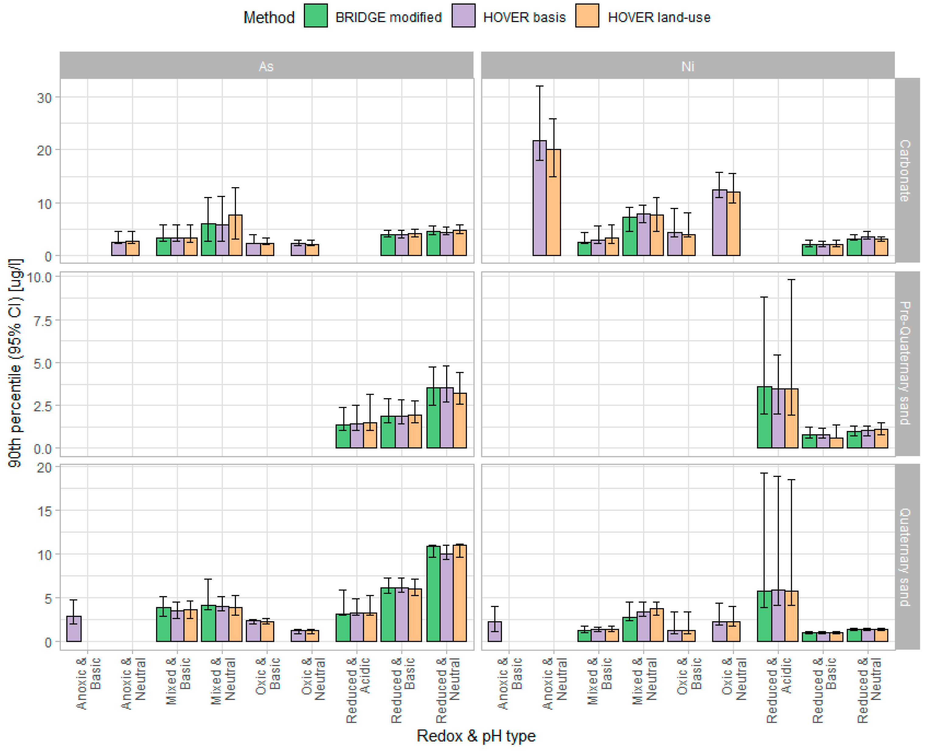
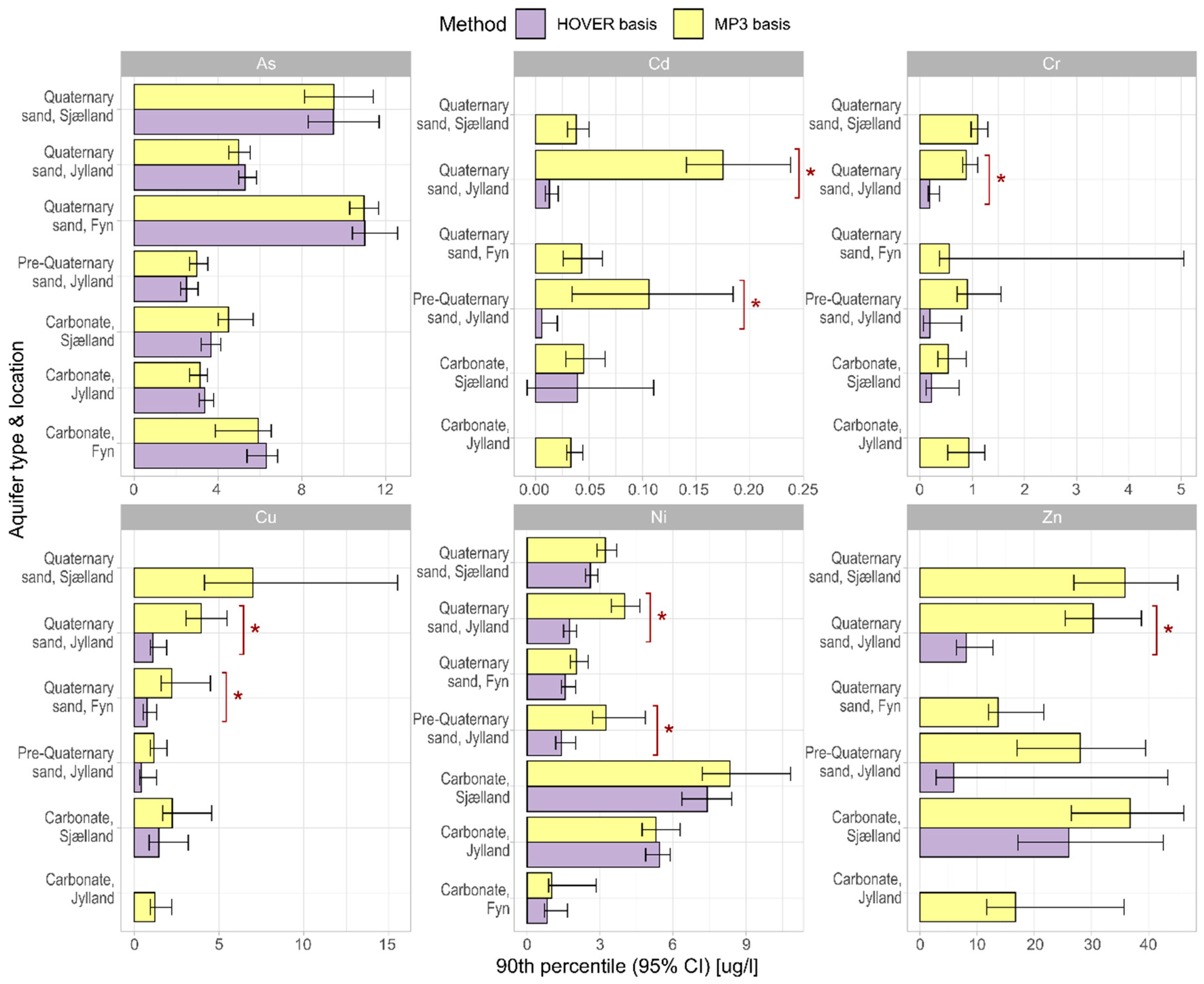
4.4. Comparison of NBLs Derived by the Different Methods

The NBLs of trace metals for the main aquifer types in Denmark, calculated based on the three methods, are compared in Figure 7. The only statistically significant difference (based on 95% CI) is for Ni in the carbonate aquifers and in the Quaternary sand, where BRIDGE modified results in lower values than HOVER basis (Figure 7). For all other types, the 95% CI is overlapping; thus, the differences are not significant. The NBLs for As in Quaternary sand exceed the national TV (5 µg/L) irrespective of the method.
We calculated NBLs considering redox and pH only for As and Ni (Figure 8) due to insufficient data for the rest of the elements. There is no significant difference between the NBLs obtained by the three methods for both Ni and As (Figure 8). The methods also agree that the NBLs for As are exceeding the national TV for carbonate aquifers with mixed redox conditions and neutral pH, and for Quaternary sand aquifers with reduced conditions and basic to neutral pH.
HOVER basis and HOVER land-use agree that the NBLs for Ni exceed the national TV (10 µg/L) for carbonate aquifers with oxic/anoxic redox conditions and neutral pH. NBLs could not be derived based on the BRIDGE modified for this aquifer type as there were not enough sampling points. If the upper limit of the 95% CI is considered as well, there are few other classes with exceedance of the national TV (Tables S3 and S4).
The NBLs derived by the two versions of the basis level method (HOVER rbasis and MP3 basis) are compared in Figure 9. For this comparison, the location of the aquifer (Jylland, Sjælland, Fyn, Figure 1a) was also considered. This is how the aquifer types were defined in MP3 [14], so to compare NBLs, we had to apply the same classification with the HOVER basis dataset. The following statistically significant differences in NBLs are observed:
  • Quaternary sand aquifers on Jylland—Cd, Cr, Cu, Ni, and Zn;
  • Quaternary sand aquifers on Fyn—Cu;
  • Pre-quaternary sand aquifers on Jylland—Cd, Ni.
The two methods agree that the NBLs for As are exceeding the national TV for Quaternary sand, irrespective of the location (Fyn > Sjælland > Jylland). The NBL for Ni in carbonate aquifers on Sjælland is also elevated in comparison to those on Jylland and Fyn, but it does not exceed the national TV (10 µg/L). The upper confidence limit for MP3 basis is, however, exceeding it.

5. Discussion

5.1. Comparative Analysis of the Tested Methods

Table 4 summarizes our experience with the three methods for excluding anthropogenically influenced sampling points. The summary is organized into three categories: Requirements, advantages, and disadvantages.
The NBLs resulting from these three methods (Figure 7 and Figure 8) did not differ significantly at the 95% CI. This could indicate that as a whole HOVER basis dataset was not affected by pollution in a significant way. The only exception was for Ni in the carbonate and Quaternary sand aquifers where BRIDGE modified resulted in lower NBLs than HOVER basis. These lower NBLs for Ni could arise because many of the excluded NO3-containing sampling points (>10 mg/L) also had high Ni concentrations. Figure 8 shows that the highest NBLs for Ni for both HOVER basis and land-use are found in anoxic carbonate aquifers with neutral pH; however, no NBLs could be computed for BRIDGE modified due to the additional exclusion of sampling points with NO3 > 10 mg/L.
The primary source of elevated Ni concentrations in Danish groundwater has been linked to the release of Ni during pyrite oxidation due to lowering of the water table due to abstraction or changes in the barometric pressure causing barometric pumping in the vicinity of the well [15,16,17]. Some of the Ni is then demobilized due to sorption on carbonate sediments, with rates dependent on the relative clay content of the sediment [16,17]. When the groundwater level is re-established, this secondary pool of Ni is also mobilized due to ion exchange with Ca-containing groundwater [17]. It was also shown that the elevated groundwater concentrations of Ni in eastern Sjælland (Figure 4b) were due to Ni mobilization over short distances (<500 m) rather than due to a regional groundwater transport issue [17]. When assessing the groundwater bodies’ status in MP3, the NBLs exceeding the national TVs were used instead of the national TV (i.e., a new TV was set to be equal to the NBL). However, because of this documented process of anthropogenic influence, the NBLs for Sjælland were not used when the NBLs of Ni were established as part of the MP3.
The second comparison was between the two basis level methods, which included only pre-selection of sampling points (HOVER basis and MP3 basis). The observed differences in NBLs between the HOVER basis and MP3 basis can be attributed to the cumulative effect of the different methodological specifics (Table 2). To isolate the effect of the different period and aggregation method (median vs. mean of the annual means, MAM), we compared the two datasets, including only the sampling points present in both datasets (see Figure S7). The representative concentrations at sampling points based on the MAM aggregation are overall higher than the aggregation based on a median (Figure S7). The difference is negligible for As and Ni, but for Cd, Cr, Cu, and Zn, it is substantial (Figure S7).
The wells’ pre-selection did not affect the NBLs for As, but there are significant differences for all other elements (Figure 9). It is possible that the observed significant differences could be because the MP3 basis dataset also includes water sampling points representing the shallower groundwater bodies. When the depth of the sampling points included in MP3 basis and HOVER basis datasets are compared, the median top/bottom of the abstraction screens are at 34/46 m below terrain for MP3 basis, while they are at 39/53 m below terrain for HOVER basis. However, further studies are needed to evaluate the effect of potential leaching of trace metals from the agricultural topsoil to the shallow groundwater resources.
The relative size of anthropogenic sources of trace metals to Danish soils was estimated in the early 90s based on a nationwide dataset of their content in the top-25 cm (regular grid n = 393, 1992) [32]. The levels of Ni, Zn, and Cr in soil were attributed to mainly natural sources (high correlation with soil texture and small difference between land-use), while anthropogenic sources were influencing the levels of Cd, Cu, and As [32]. The soil monitoring campaign was repeated in 2014 [8] and uncovered a significant increase in both Cu (36%) and Zn (41%) concentrations in the topsoil. Their primary sources on arable land in Denmark come from the use of organic fertilizers such as manure, slurry, and sewage sludge [8]. Cu and Zn can reach high concentrations in manure and slurry due to their use as growth-promoting additives in livestock feed and their use in the prevention of diarrhea associated with E. coli [8].
Selecting only the drinking water wells (as in HOVER basis) limits the representativity of the dataset to only groundwater types abstracted for drinking water purposes. Next to limiting representativity, it also limited the data availability for Cd, Cr, Cu, and Zn (Table 3) and, respectively, the ability to derive NBLs for different hydrogeochemical conditions (Figure 8) or different aquifer locations (Figure 9). Considering these limitations, we can conclude that including the wells from the national groundwater monitoring network, as in MP3 basis, improves the data availability and representativity of the NBLs (with respect to the shallow groundwaters), but also results in higher NBL for most of the studied trace metals.

5.2. Other Possibilities for Assessing Anthropogenic Influences

The original BRIDGE method [4] also included a condition for identifying hydrothermal, brackish/saline groundwaters, based on the concentrations of Na and Cl ions ([Na+] + [Cl] > 1000 mg/L). Hydrothermal waters are not characteristic for Denmark, and in addition to that, groundwater used for drinking water purposes usually has low salinity, as it should comply with the national and EU drinking water standards for Cl (250 mg/L) and Na (175 mg/L) (BEK nr 1070 af 28/10/2019). There was Cl and Na data for 99.7% of all sampling points included in the HOVER basis dataset. The sum of Na and Cl exceeded 1000 mg/L for only two of the sampling points, but both of those had low median As (0.04 µg/L and 0.045 µg/L) and Ni (0.3 µg/L and 0.045 µg/L). Thus, we decided that this condition is not relevant for our study, so we kept only the NO3 condition of the original BRIDGE method [2] and modified the method by adding other pollution indicators (pesticides and organic micropollutants).
Another possibility for assessing the anthropogenic influence due to unsustainable pumping practices, characteristic for some urbanized areas in Denmark, is performing Cl and SO4 trend analysis. Increasing Cl trends are indicative for saltwater intrusion (due to sea-water intrusion or up-coning of deeper saline groundwater) and potential lowering of the groundwater table. Linear trend analysis for Cl and SO4 was performed for 92 groundwater bodies at risk of bad quantitative state for MP3 [21]. However, there was only enough data (min 8 y of data at sampling points in 1988–2016) for 26% of these groundwater bodies, most of which are located on Sjælland and Fyn [21]. If we consider the sampling points included in the HOVER basis dataset, Cl and SO4 trends [21] are available for 297 or 253, respectively. Of those, 43.8% had significant (p < 0.05) increasing Cl trends, and 32.8% significantly increasing SO4 trends. As there were no high Cl concentrations, the effect of marine conditions is minor even with increasing Cl trends. Using Cl and SO4 trends is limited by data availability and requires in-depth assessment at the groundwater body level, which is beyond the scope of this study. However, understanding the impacts of groundwater abstraction is relevant, especially in areas with urban anthropogenic pressures where long-term trends in different water quality parameters could be used as indicators for unsustainable aquifer exploitation [33].
Groundwater age could be another potential indicator, where the older (“pre-industrial”) groundwaters [34] would be representing the baseline groundwater quality. An example of such a study in New Zealand can be found in [35]. Unfortunately, groundwater age (CFC-based) could be determined only for 69 of the sampling points of the HOVER basis dataset. Only a few waterworks in Denmark have dated the groundwater of their abstraction wells, and even fewer have reported it to Jupiter. In addition, the groundwater abstracted from long filters can be a mixture of very different ages [36], and the CFC in most waterworks wells can be expected to be partly degraded due to the reduced conditions [37]. Tritium data was also available for only a few of the sampling points (n = 58). If combined, there were in total 125 sampling points with either CFC or tritium data; thus, due to this low data coverage, we deemed this method as inappropriate for the current study. In future studies, if the pre-selection of wells was extended to the groundwater monitoring wells (as in MP3) or all wells that have been dated, this method should also be explored.

5.3. Implications and Recommendations

According to EU policies and guidelines [1,2,3,13], NBLs derived for groundwater bodies should be used by the national authorities of EU member states to derive and establish TVs based on criteria values for legitimate groundwater uses (e.g., drinking water) and the environment to protect human health and the ecological status of dependent terrestrial and associated aquatic ecosystems. Hence, the selected methods for the derivation of NBLs have important implications for the protection of human health, ecosystems, and biodiversity across Europe. Based on the NBL analyses presented in this study for Denmark—a country with intensive agriculture and widespread anthropogenic pressures—we prepared the following roadmap for method selection when determining NBLs for trace elements (Figure 10). This roadmap is applicable for NBL derivation at the national scale in countries with varying amounts of data, and it can be adjusted based on the local hydrogeological and hydrogeochemical conditions. Our assessment was based on aquifer types (groups of groundwater bodies) representing carbonate aquifers, Quaternary and pre-Quaternary sand aquifers, and their pH and redox conditions. However, the definitions of aquifer types should be adjusted to suit best the local conditions and data availability. The pre-selection of sampling points based on the primary use of the well or the sampling purpose is an important step in assuring that anthropogenically influenced points are removed from the dataset. However, this “cleaning” of the dataset should be performed with attention to the representativity and data availability, as well.

6. Conclusions

We developed a roadmap for deriving NBLs for trace metals (As, Cd, Cr, Cu, Ni, Zn), in the context of intensive and widespread agriculture and extensive groundwater pumping for drinking water supply in urban areas. This work contributes to the need for harmonization in the NBL derivation by EU member states for the purposes of assessing the chemical status of groundwater bodies stipulated by the WFD and GWD. It provides a systematic way of selecting an appropriate method or combination of methods to assure that NBLs are calculated based on groundwater data representing no or only very minor anthropogenic alterations to undisturbed conditions.
We applied and compared three different methods for excluding anthropogenically influenced sampling points: HOVER basis, HOVER land-use, and BRIDGE modified. Denmark was used as an example of a country with widespread agricultural pressures (diffuse pollution). We found that the HOVER basis provided already a relatively “clean” dataset; thus, the two other methods that removed additional sampling points potentially affected by anthropogenic pollution (HOVER land-use and BRIDGE modified) did not result in significantly different NBLs, except for Ni, for which BRIDGE modified performed best (resulted in lower NBL). Data availability limited the derivation of NBLs, accounting also for the redox and pH conditions, except for As and Ni.
Furthermore, we critically assessed these three methods, i.e., we discussed the specific data requirements, the advantages, and the disadvantages of the individual methods. This critical assessment generalizes the outcomes of our study and will hopefully help other researchers or water managers when setting NBLs for trace metals in groundwater at the national scale. We demonstrated how combining several methods and using several types of data may compensate for the individual limitations of the methods. Since the methods have different data availability requirements, the roadmap accounts for this too. Our results showed that the simplest of the three methods performed well in almost all cases, stressing the importance of excluding known polluted water sampling points. In the Danish case, this was possible because the sampling purpose and the well use are known. Thus, we recommend, if this information is available, to use it for initial pre-screening of the datasets.

Supplementary Materials

The following are available online at https://0-www-mdpi-com.brum.beds.ac.uk/article/10.3390/w13091267/s1, one file including supplementary text, and the following figures, and tables: Figure S1: Map with landscape types and the pre-quaternary stratigraphic succession in Denmark, Figure S2: Maps with sampling points classified based on aquifer type and prevailing anthropogenic pressure, Figure S3: ECDFs for the trace elements stratified by aquifer type, Figure S4: ECDFs for the trace elements stratified by pH class, Figure S5: ECDFs for the trace elements stratified by redox class, Figure S6: ECDFs for the trace elements stratified by prevailing anthropogenic pressure, Figure S7: Comparison between HOVER basis and MP3 basis datasets, Table S1: Excluded analyses during quality control, Table S2: NBLs for the trace elements in the main aquifer types based on BRIDGE modified, HOVER basis and HOVER land-use, Table S3: NBLs for As in different aquifer types based on redox, pH, and geology for the 3 methods, Table S4: NBLs for Ni in different aquifer types based on redox, pH, and geology for the 3 methods, Table S5: NBLs for trace elements for different aquifer types and locations, based on HOVER basis and MP3 basis.

Author Contributions

Conceptualization, D.D.V., L.T., V.E. and K.H.; methodology, D.D.V.; validation, J.S. and L.T.; data curation, D.D.V.; writing—original draft preparation, D.D.V.; visualization, D.D.V.; supervision, L.T., V.E., B.H. and K.H.; project administration and funding acquisition, K.H. All authors participated in the writing, review, and editing of the manuscript. All authors have read and agreed to the published version of the manuscript.

Funding

This project has received funding from the European Research Council (ERC) under the European Union’s Horizon 2020 research and innovation program (grant agreement n° 731166) and by the Innovation Fund Denmark, funding agreement number 8055-00073B.

Institutional Review Board Statement

Not applicable.

Informed Consent Statement

Not applicable.

Data Availability Statement

The raw data used in this study is publicly available in the Danish national well database (Jupiter). This data can be found here: https://eng.geus.dk/products-services-facilities/data-and-maps/national-well-database-jupiter (accessed on 29 April 2021).

Acknowledgments

This work was carried out under work package 3 of the GeoERA project HOVER; we would like to thank all our colleagues from the European geological surveys participating in this work package, especially for everyone involved in Task 3-3. The HOVER land-use method presented in this paper is an adaptation of the original method proposed by Eline Malcuit and Laurence Gourcy (BRGM) [18]. We also thank the Danish EPA for including us in the River Basin Management Plan work on assessing the status of groundwater bodies for trace elements, which allowed us to focus our attention on the practical side of NBLs derivation.

Conflicts of Interest

The authors declare no conflict of interest. The funders had no role in the design of the study; in the collection, analyses, or interpretation of data; in the writing of the manuscript; or in the decision to publish the results.

Appendix A

General guideline for establishing TVs, according to Annex II.A of GWD [2]:
“…
(1) 
the determination of TVs should be based on:
-
the extent of interactions between groundwater and associated aquatic and dependent terrestrial ecosystems;
-
the interference with actual or potential legitimate uses or functions of groundwater;
-
all pollutants which characterise bodies of groundwater as being at risk…
-
hydrogeological characteristics including information on background levels and water balance;
(2) 
the determination of [TVs] should also take into account the origins of the pollutants, their possible natural occurrence, their toxicology and dispersion tendency, their persistence and their bioaccumulation potential;…
(3) 
wherever elevated background levels of substances or ions or their indicators occur due to natural hydrogeological reasons, these background levels in the relevant body of groundwater shall be taken into account when establishing threshold values”.
Table A1. Geogenic and anthropogenic sources and geochemical controls (summarized from [5,19]).
Arsenic (As)GeogenicSulfide minerals (e.g., pyrite, arsenopyrite, arsenian pyrite); feldspars; phosphate minerals 1; sorbs to clays, Fe oxyhydroxides, and OM;
AnthropogenicPesticides; pig and poultry farming; combustion processes; ore roasting;
ControlspH and redox dependent; reductive dissolution and desorption (sulfide minerals); oxidation reactions (iron oxides)
Cadmium (Cd)GeogenicSphalerite 2; micas, amphiboles; phosphorite; due to affinity to OM, enrichment in coal and peat; sorbs to calcite surfaces, clay minerals, and OM
AnthropogenicFertilizers; sewage sludge; traffic (wear of tires); incinerators; coal combustion; metal smelters; iron and steel mills; electroplating
ControlspH and redox dependent; soluble in oxidizing conditions at pH < 8; co-precipitates with Fe and Mn hydroxides
Chromium (Cr)GeogenicFerromagnesian minerals (e.g., olivine, pyroxene, amphibole); micas; garnets; enriched in mafic and ultramafic rocks, shales, and other argillaceous rocks; sorbs to clays, Fe and Mn oxyhydroxides, and OM
AnthropogenicTanning and wood impregnation; steel industry;
ControlspH and redox dependant; mobile under acidic oxidizing conditions and forms inorganic and organic complexes
Copper (Cu)GeogenicSulfide minerals (e.g., chalcopyrite); accessory in many common minerals (e.g., micas and amphiboles); strong sorption to OM, Fe, and Mn oxyhydroxides;
AnthropogenicFarm effluents and sewage sludge 3; wide range of industrial and urban uses (e.g., roofing, pipework, plumbing, and water components; electrical industry);
ControlspH and redox dependant; highest mobility under acidic and oxidizing conditions; forms inorganic and organic complexes; co-precipitates with Fe and Mn hydroxides
Nickel (Ni)GeogenicNi-minerals; accessory in sulfide minerals (e.g., pyrite, chalkopyrite) and other common minerals (e.g., micas and amphiboles); closely associated with Cr and Co; sorbs to Fe and Mn oxides, clay edges, calcite
AnthropogenicPhosphate fertilizers (“contaminant” along with Zn, Cr, and Cd);
industrial and urban pollution (alloys, batteries, magnets, plating, pigments); landfill leachates
ControlspH and redox dependant 4; highly mobile under acidic and reducing conditions; in near-neutral waters, it may form carbonate complexes
Zinc (Zn)GeogenicSphalerite; range of Zn-carbonates (e.g., smithsonite) and oxides; can be present as a trace constituent in calcite; in clays, it may be in secondary oxide and silicate minerals; sorbs to oxide and oxyhydroxide minerals
AnthropogenicUsed as anticorrosion coating of steel, in alloys, pipework, plumbing, and water components; pigment in paint; in rubber products
ControlspH and redox dependant 5; highest mobility under acidic and oxidizing conditions; mobile also in circum-neutral and alkaline conditions
1 possible substitution of P5+ with As5+ [19]; 2 Cd could be replacing 0.5% and up to 1.5% of the Zn [19]; 3 Cu may be administered as a supplement to farm animals [19]; 4 Ni is not redox-sensitive, but it is affected by redox processes as the redox-sensitive elements Mn and Fe are linked with its mobilization in water; 5 Zn has only one oxidation state, so insensitive to redox, but its ability to be adsorbed to metal oxyhydroxides may have indirect control.
Table A2. Groundwater sampling points in each class; the dominating classes are shown in bold.
AsCdCuCrNiZn
HOVER basis dataset (n)63523552892506358363
Aquifer type (%)
• Carbonate352324233524
•  Quaternary sand535764645356
• Pre-Quaternary sand101612121015
• Bornholm (various)15--15
pH class (%)
• Acidic554356
• Basic272627302727
•  Neutral575756535755
• Unknown101212141012
Redox class (%)
• Oxic855484
• Anoxic432343
•  Reduced768182827682
• Mixed131110111310
• Unknown<1---<1<1
Prevailing pressure (%)
•  Agricultural868175758677
• Industrial152315
• Urban131522221317
• Mining<1---<1-
• No pressure (natural)1-<1-1<1

References

  1. European Commission. Directive 2000/60/EC of the European Parliament and of the Council, of 23 October 2000, establishing a framework for community action in the field of water policy. Off. J. Eur. Communities 2000, 327, 1–73. [Google Scholar]
  2. European Commission. Directive 2006/118/EC of the European Parliament and of the Council of 12 December 2006 on the Protection of Groundwater against Pollution and Deterioration. Off. J. Eur. Union 2006, 372, 19–31. [Google Scholar]
  3. European Commission. Guidance on Groundwater Status and Trend Assessment (Guidance Document No. 18 of the Common Implementation Strategy for the Water Framework Directive (2000/60/EC); Technical Report; Office for Official Publications of the European Communities: Luxembourg, 2009; ISBN 978-92-79-11374-1. [Google Scholar]
  4. Hinsby, K.; Condesso de Melo, M.T.; Dahl, M. European case studies supporting the derivation of natural background levels and groundwater threshold values for the protection of dependent ecosystems and human health. Sci. Total Environ. 2008, 401, 1–20. [Google Scholar] [CrossRef] [PubMed]
  5. Edmunds, W.M.; Shand, P. (Eds.) Natural Groundwater Quality; Blackwell Pub: Malden, MA, USA, 2008; ISBN 978-1-4051-5675-2. [Google Scholar]
  6. Scheidleder, A. Groundwater Threshold Values: In-Depth Assessment of the Differences in Groundwater Threshold Values Established by Member States; Umweltbundesamt (Environment Agency Austria): Vienna, Austria, 2012; p. 57. [Google Scholar]
  7. EC; CIS Working Group Groundwater. Threshold Values—Initial Analysis of 2015 Questionnaire Responses; European Commission: Brussels, Belgium, 2015; p. 46. [Google Scholar]
  8. Jensen, J.; Larsen, M.M.; Bak, J. National monitoring study in denmark finds increased and critical levels of copper and zinc in arable soils fertilized with pig slurry. Environ. Pollut. 2016, 214, 334–340. [Google Scholar] [CrossRef] [PubMed]
  9. Koch, J.; Stisen, S.; Refsgaard, J.C.; Ernstsen, V.; Jakobsen, P.R.; Højberg, A.L. Modeling depth of the redox interface at high resolution at national scale using random forest and residual gaussian simulation. Water Resour. Res. 2019, 55, 1451–1469. [Google Scholar] [CrossRef]
  10. Frei, R.; Frei, K.M.; Kristiansen, S.M.; Jessen, S.; Schullehner, J.; Hansen, B. The link between surface water and groundwater-based drinking water—Strontium isotope spatial distribution patterns and their relationships to Danish sediments. Appl. Geochem. 2020, 121, 104698. [Google Scholar] [CrossRef]
  11. Sandersen, P.B.E.; Jørgensen, F. Buried tunnel valleys in Denmark and their impact on the geological architecture of the subsurface. GEUS Bull. 2017, 38, 13–16. [Google Scholar] [CrossRef]
  12. Troldborg, L. Afgrænsning af de Danske Grundvandsforekomster: Ny Afgrænsning og Delkarakterisering Samt Fagligt Grundlag for Udpegning af Drikkevandsforekomster; GEUS Rapport 2020/1; Geological Survey of Denmark and Greenland (GEUS): Copenhagen, Denmark, 2020; p. 82. (In Danish) [Google Scholar]
  13. European Commission. Council Directive 98/83/EC of 3 November 1998 on the Quality of Water Intended for Human Consumption. Off. J. Eur. Union 2015, 330, 32–54. Available online: http://data.europa.eu/eli/dir/1998/83/2015-10-27 (accessed on 29 April 2021).
  14. Ernstsen, V.; Mortensen, M.H.; Voutchkova, D.D.; Thorling, L. Udvikling af Metode til Vurdering af Grundvandsforekomsters Kemiske Tilstand for Udvalgte Uorganiske Sporstoffer og Salte; GEUS Rapport 2021/19; Geological Survey of Denmark and Greenland (GEUS): Copenhagen, Denmark, 2020. (In Danish) [Google Scholar]
  15. Larsen, F.; Postma, D. Nickel mobilization in a groundwater well field: Release by pyrite oxidation and desorption from manganese oxides. Environ. Sci. Technol. 1997, 31, 2589–2595. [Google Scholar] [CrossRef]
  16. Jensen, T.F.; Larsen, F.; Kjøller, C.; Larsen, J.W. Nikkelfrigivelse ved Pyritoxidation Forårsaget af Barometerånding—Pumpning; Arbejdsrapport 5; Miljøstyrelsen: Odense, Denmark, 2003; p. 131. (In Danish) [Google Scholar]
  17. Kjøller, C.; Jessen, S.; Larsen, F.; Postma, D.; Jakobsen, R. Binding af Nikkel til og Frigivelse fra Naturlige Kalksedimenter; Arbejdsrapport 8; Miljøstyrelsen: Odense, Denmark, 2006; p. 144. (In Danish) [Google Scholar]
  18. Lions, J.; Malcuit, E.; Gourcy, L.; Voutchkova, D.; Hansen, B.; Schullehner, J.; Forcada, E.G.; Olmedo, J.G.; Elster, D.; Camps, V.; et al. Proposing a Common Methodology to Calculate the Natural Concentration of Dissolved Elements Based on Lithological/Geological Water Families Taking into Account Possible Anthropogenic Influences; Report type Deliverable of HOVER Project No. D 3-3; 2021; p. 206. [Google Scholar]
  19. Reimann, C.; Birke, M. (Eds.) Geochemistry of European Bottled Water; Borntraeger Science Publishers: Stuttgart, Germany, 2010; ISBN 978-3-443-01067-6. [Google Scholar]
  20. Thorling, L.; Ditlefsen, C.; Ernstsen, V.; Hansen, B.; Johnsen, A.R.; Troldborg, L. Grundvandovervågning. Status og Udvikling 1989–2018; Teknisk Rapport; Geological Survey of Denmark and Greenland (GEUS): Copenhagen, Denmark, 2019; p. 132. (In Danish) [Google Scholar]
  21. Henriksen, H.J.; Voutchkova, D.; Troldborg, L.; Ondracek, M.; Schullehner, J.; Hansen, B. National Vandressource Model. Beregning af Udnyttelsesgrader, Afsænkning og Vandløbspåvirkning Med DK Model 2019; GEUS Rapport 2019/32; Geological Survey of Denmark and Greenland (GEUS): Copenhagen, Denmark, 2019; p. 84. (In Danish) [Google Scholar]
  22. R Core Team. R: A Language and Environment for Statistical Computing; R Foundation for Statistical Computing: Vienna, Austria, 2020. [Google Scholar]
  23. Hyndman, R.J.; Fan, Y. Sample quantiles in statistical packages. Am. Stat. 1996, 50, 361. [Google Scholar] [CrossRef]
  24. Millard, S. EnvStats: An R Package for Environmental Statistics; R Package; Springer: New York, NY, USA, 2013; ISBN 978-1-4614-8455-4. [Google Scholar]
  25. Wickham, H. Stringr: Simple, Consistent Wrappers for Common String Operations; R Package. 2019. Available online: https://CRAN.R-project.org/package=stringr (accessed on 5 January 2021).
  26. Wickham, H. Ggplot2: Elegant Graphics for Data Analysis; R Package; Springer: New York, NY, USA, 2016; ISBN 978-3-319-24277-4. [Google Scholar]
  27. Wickham, H. Tidyr: Tidy Messy Data; R Package. 2020. Available online: https://CRAN.R-project.org/package=tidyr (accessed on 5 January 2021).
  28. Wickham, H.; François, R.; Henry, L.; Müller, K. Dplyr: A Grammar of Data Manipulation; R Package. 2020. Available online: https://CRAN.R-project.org/package=dplyr (accessed on 5 January 2021).
  29. Dowle, M.; Srinivasan, A. Data.Table: Extension of ‘Data.Frame’; R Package. 2020. Available online: https://CRAN.R-project.org/package=data.table (accessed on 5 January 2021).
  30. QGIS Development Team. QGIS Geographic Information System; Long Term Release; QGIS Association. 2021. Available online: https://qgis.org/en/site/ (accessed on 5 January 2021).
  31. Inkscape’s Contributors. Inkscape—A Free and Open Source Vector Graphics Editor; The Inkscape Project. 2021. Available online: https://inkscape.org/ (accessed on 5 January 2021).
  32. Bak, J.; Jensen, J.; Larsen, M.M.; Pritzl, G.; Scott-Fordsmand, J. A heavy metal monitoring-programme in Denmark. Sci. Total Environ. 1997, 207, 179–186. [Google Scholar] [CrossRef]
  33. Gejl, R.N.; Rygaard, M.; Henriksen, H.J.; Rasmussen, J.; Bjerg, P.L. Understanding the impacts of groundwater abstraction through long-term trends in water quality. Water Res. 2019, 156, 241–251. [Google Scholar] [CrossRef] [PubMed]
  34. Hinsby, K.; Edmunds, W.M.; Loosli, H.H.; Manzano, M.; Condesso De Melo, M.T.; Barbecot, F. The modern water interface: Recognition, protection and development—advance of modern waters in european aquifer systems. Geol. Soc. Lond. Spec. Publ. 2001, 189, 271–288. [Google Scholar] [CrossRef]
  35. Morgenstern, U.; Daughney, C.J. Groundwater age for identification of baseline groundwater quality and impacts of land-use intensification—The national groundwater monitoring programme of New Zealand. J. Hydrol. 2012, 456–457, 79–93. [Google Scholar] [CrossRef]
  36. Jakobsen, R.; Hinsby, K.; Aamand, J.; van der Keur, P.; Kidmose, J.; Purtschert, R.; Jurgens, B.; Sültenfuss, J.; Albers, C.N. History and sources of co-occurring pesticides in an abstraction well unraveled by age distributions of depth-specific groundwater samples. Environ. Sci. Technol. 2020, 54, 158–165. [Google Scholar] [CrossRef] [PubMed]
  37. Hinsby, K.; Højberg, A.L.; Engesgaard, P.; Jensen, K.H.; Larsen, F.; Plummer, L.N.; Busenberg, E. Transport and degradation of chlorofluorocarbons (CFCs) in the pyritic rabis creek aquifer, Denmark. Water Resour. Res. 2007, 43. [Google Scholar] [CrossRef] [Green Version]
Figure 1. (a) Land-use map (CORINE 2012, downloaded from https://download.kortforsyningen.dk/content/corine-land-cover (accessed on 20 May 2020)). (b) Groundwater bodies included in this study; the Quaternary sand is shown with transparency above the other aquifer types, so the underlying carbonate and pre-Quaternary sand aquifers can also be seen.
Water 13 01267 g001
Figure 2. Compared methods and how they relate to each other, the basis method has two versions—from the HOVER project and from the third River Basin Management Plan (MP3). The dataset from HOVER basis is further used with HOVER land-use and BRIDGE modified methods.
Water 13 01267 g002
Figure 3. Empirical distribution for As, Cd, Cr, Cu, Ni, and Zn in Danish groundwater at waterworks wells used for drinking water production; each point is a median concentration for 2009–2018 at each sampling point.
Water 13 01267 g003
Figure 4. Spatial distribution of sampling points with As (a) and Ni (b) exceeding the national threshold values for As (5 µg/L) and Ni (10 µg/L).
Water 13 01267 g004
Figure 5. Spatial distribution of the groundwater sampling points based on their pH (a) and redox (b) class.
Water 13 01267 g005
Figure 6. Location of sampling points that were excluded when calculating NBLs for the HOVER land-use (a) and the BRIDGE modified (b) methods.
Water 13 01267 g006
Figure 7. NBLs (y-axis, µg/L) for As, Cd, Cr, Cu, Ni, and Zn (see gray panel labels) based on the three methods. The symbol * indicates a statistically significant difference based on the 95% confidence intervals (CI); For values and number of sampling points, see Table S2.
Water 13 01267 g007
Figure 8. NBLs (y-axis, µg/L) for As and Ni (gray panel labels, top) considering the pH and redox (x-axis) of the aquifer types (gray panel labels, right). No significant differences are observed based on the 95% confidence interval (CI). Tables S3 and S4 provide values and number of samples.
Water 13 01267 g008
Figure 9. NBLs (x-axis, µg/L) for As, Cd, Cr, Cu, Ni, and Zn (see gray panel labels), calculated based on HOVER basis and MP3 basis methods considering the aquifer type and location (y-axis). The symbol * indicates a statistically significant difference based on the 95% confidence intervals (CI). See also Table S5 for the numbers and Figure 1 for geographical reference.
Water 13 01267 g009
Figure 10. Roadmap for determining natural background levels (NBLs) for trace elements showing the different steps in the data analysis based on data availability; the 3 methods for excluding anthropogenic influences that were tested in this study are also mapped.
Water 13 01267 g010
Table 1. Drinking water quality standard and groundwater threshold values in Denmark.
UnitAsCdCuCrNiZn
National threshold valueµg/L50.51002510100
National drinking water standardµg/L53200050203000
Table 2. Methodology comparison for NBL assessment based on the HOVER and MP3.
MethodHOVER BasisMP3 BasisComparison
Data source[20]Same
Sampling pointsWaterworks wellsWaterworks and monitoring wellsOverlap
Period2009–2018 (incl.)2000–2018 (incl.) [a]Overlap
Limit of detection<LOD = 1.5 × LODSame [b]
Aggregation (intake)MedianMean of annual meansDifferent
Aquifer types:
- GeologyCarbonates, pre-Quaternary sand, Quaternary sand, DiverseSame
- Location-Jylland, Sjælland, Fyn, BornholmDifferent
- pHAcidic, neutral, basicLow, highDifferent
- RedoxOxic, anoxic, reduced, mixed Oxic, anoxicDifferent
- Organic matter-high, lowDifferent
Representativeness [c]20 (30)/50Same
NBL computation90th percentileSame
Target spatial scale and usePan-European and non-regulatoryNational and regulatoryOverlap
[a] trace elements data for this period, but only for sampling points that could be classified into pH, redox, NVOC classes based on data for 2009–2018; [b] MP3 had more stringent exclusion of data with high detection limits; [c] minimum number of sampling points for aquifer type to calculate NBL.
Table 3. Groundwater sampling points in the datasets after excluding the anthropogenically influenced points.
nAsCdCrCuNiZn
HOVER basis63523552502896358363
HOVER land-use55083372412855558359
BRIDGE modified54102972082395414300
MP3 basis56711666913142456721689
Table 4. Comparative analysis for HOVER basis, HOVER land-use, and BRIDGE modified.
HOVER basisRequirementsAvailability of information about the sampling purpose, enabling exclusion of sampling points used for monitoring of polluted sites (as a minimum). Meta-data for most sampling points in Denmark is available in the Jupiter database.
AdvantagesLow data and labor intensity
DisadvantagesThe anthropogenic pressures are not assessed directly. Data from polluted yet active waterworks wells may be present in the data set. The data set is not representative for all groundwater types, only for those favored for drinking water abstraction and supply.
HOVER land-useRequirementsMapping prevailing anthropogenic pressures in the catchment of the well (recharge zone) in GIS software.
AdvantagesModerately data and labor-intensive, CORINE land cover can be downloaded freely from https://land.copernicus.eu/pan-european/corine-land-cover (accessed on 29 April 2021).
DisadvantagesAnthropogenic pressure in the catchment does not necessarily result in groundwater pollution. Other factors are not considered.
The catchments (or groundwater recharge zones) are unknown for all wells at the national scale. The approximation of a 1 km buffer around the well may under- or overrepresent the actual area. No delineation between intensive/extensive/organic agriculture is included. All anthropogenic pressures were given equal weight, and only their areal proportions mattered when assigning prevailing pressure to each well. The proximity to roads was not included in the analysis, even though storm runoff may contribute to heavy metal loads. The method can only be applied partially if there are no representative sampling points without anthropogenic pressures (prevailing natural areas).
BRIDGE modifiedRequirementsAvailability of groundwater quality data for other chemical compounds indicating anthropogenic pressure from agricultural activities (e.g., nitrate, pesticides) or urban/industrial activities (e.g., organic micropollutants).
AdvantagesA more holistic assessment of potential pollution as opposed to basing the analysis on a single trace element at a time.
DisadvantagesVery data and labor-intensive if it is done on a national scale.
The NO3 condition limits the assessment to aquifer types with reduced conditions mostly. The sampling points representing shallow, oxidized groundwater below agricultural land with NO3 > 10 mg/L are excluded from the dataset, which in the Danish conditions means that NBLs for the shallow oxic and anoxic aquifers cannot be derived by this method, as those water types are mostly affected by diffuse pollution. However, any method that provides NBLs for such water types must be carefully analyzed and tested with independent data. In addition, this method is not particularly suitable for screening against industrial or mining pollution when only heavy metals are released into the groundwater, as other pollution indicators are used here.
Publisher’s Note: MDPI stays neutral with regard to jurisdictional claims in published maps and institutional affiliations.

