
Air–Water Properties in Rectangular Free-Falling Jets


1
Hidr@m Group, Department of Mining and Civil Engineering, Universidad Politécnica de Cartagena, 30203 Cartagena, Spain
2
Civil and Environmental Engineering Department, Escuela Politécnica Nacional, Quito 170517, Ecuador
*
Author to whom correspondence should be addressed.
Water 2021, 13(11), 1593; https://0-doi-org.brum.beds.ac.uk/10.3390/w13111593
Submission received: 16 April 2021
/
Revised: 1 June 2021
/
Accepted: 3 June 2021
/
Published: 5 June 2021
(This article belongs to the Special Issue Advances in Spillway Hydraulics: From Theory to Practice)
Abstract
:This study analyzes the air–water flow properties in overflow nappe jets. Data were measured in several cross-sections of rectangular free-falling jets downstream of a sharp-crested weir, with a maximum fall distance of 2.0 m. The flow properties were obtained using a conductivity phase-detection probe. Furthermore, a back-flushing Pitot-Prandtl probe was used in order to obtain the velocity profiles. Five specific flows rates were analyzed, from 0.024 to 0.096 m3/s/m. The measurements of the air–water flow allowed us to characterize the increment of the air entrainment during the fall, affecting the flow characteristic distributions, reducing the non-aerated water inner core, and increasing the lateral spread, thereby leading to changes in the jet thickness. The results showed slight differences between the upper and lower nappe trajectories. The experimental data of the jet thickness related to a local void fraction of 50% seemed to be similar to the jet thickness due only to gravitational effects until the break-up length was reached. The amount of energy tended to remain constant until the falling distance was over 15 times greater than the total energy head over the weir crest, a distance at which the entrained air affected the entire cross-section, and the non-aerated core tended to disappear. The new experiments related with air–water properties in free-falling jets allow us to improve the current knowledge of turbulent rectangular jets.
1. Introduction
During the latter part of the 20th century and into the 21st century, updated hydrological time-series data and new dam safety regulations have required the reevaluation of spillways’ capacity and hydraulic structures in large dams. Many studies have raised concerns that the current discharge capacity of several hydraulic structures may be insufficient for extreme events, and that those structures may suffer uncontrolled overflow scenarios, thus compromising the stability and safety of the structure (FEMA [1]). Those new situations create new questions about the hydrodynamic actions at the toe of the dams (Wahl et al. [2]).
Free-falling water jets in arch dams produce air entrainment and energy dissipation, which change the flow properties. Those types of high-velocity air–water flows are characterized by turbulent mixing processes and large amounts of entrained air (Felder and Chanson [3]).
2. Previous Studies
According to Ervine and Falvey [4], the air-entrainment mechanisms in jets are due to the turbulence; to overcome the stabilization forces of the surface tension and the buoyancy effects, the turbulent shear stress should be large enough to disturb the surface. At the beginning, the internal turbulence forms small undulations and instabilities on the free surface. Later, eddies in the turbulent jets are of the same order of magnitude as the perturbation amplitude in the surface. Then, waves and instabilities are amplified in the flow direction, and turbulence instabilities affect the free surface. Finally, the non-aerated core of the jet is affected by the large turbulent fluctuations. Hence, surface disturbances are related with the turbulent kinetic energy jet.
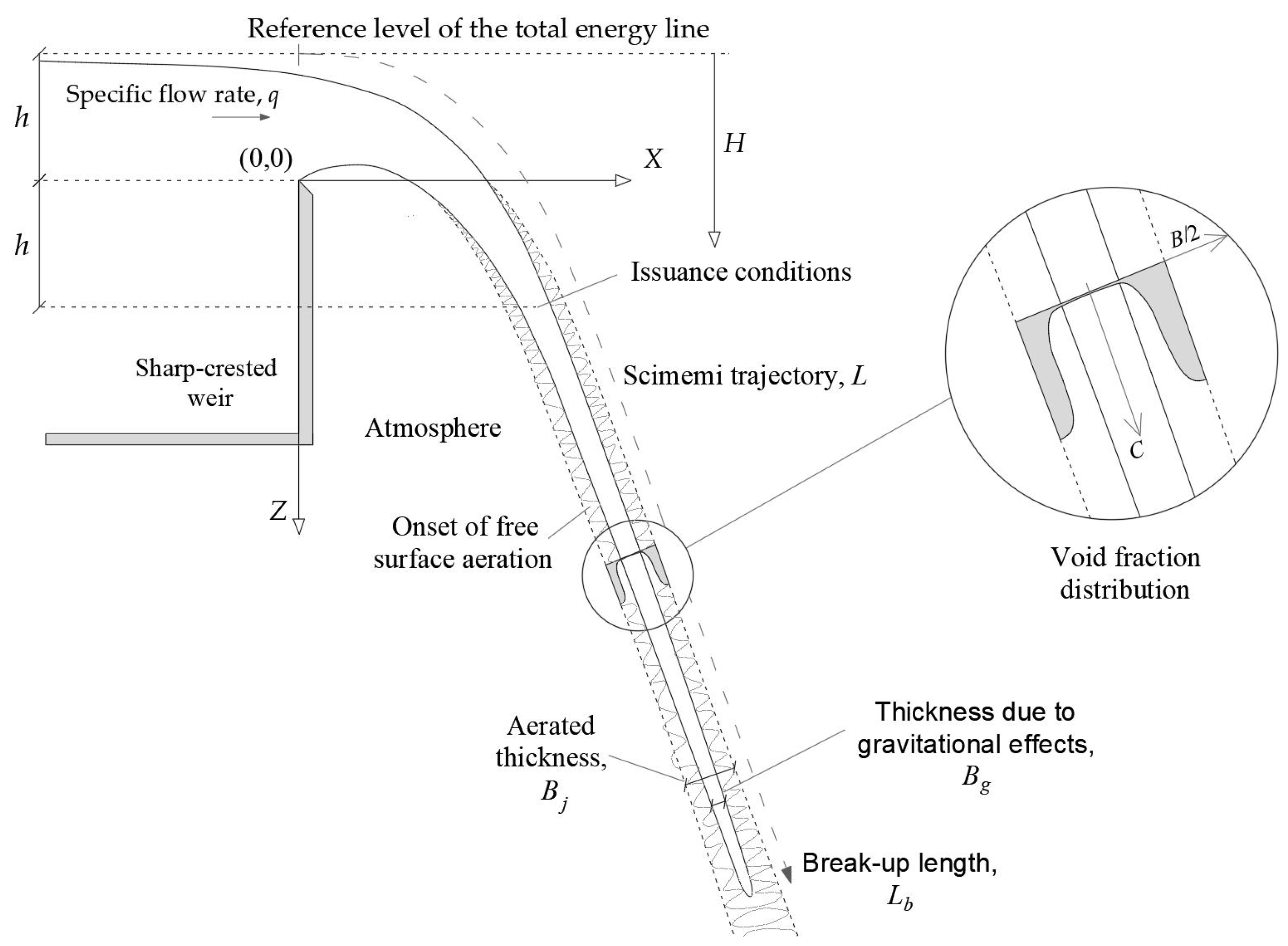
Following Castillo et al. [5], the energy mechanism in nappe jets may be divided into different steps: (1) self-aeration and spreading of the jet during the fall, (2) air entrainment and diffusion of the plunging jet in the water cushion, (3) impact of the jet with the bottom of the plunge pool, and (4) recirculation and diffusion in the submerged hydraulic jump. The air–water characteristics of the falling jets may play an important role in the air entrainment and energy dissipation in plunge pools (Bertola et al. [6]). Figure 1 shows a representation of the spreading in rectangular free-falling jets. The scheme was adapted from those presented by Ervine and Falvey [4], who reported inner core decay angles around 0.5–1% (excluding the gravitational effect) and outer spread angles around 2–5% in circular falling jets measured in a device that generated vertical trajectory jets.
The air entrainment in free-falling jets modifies the theoretical flow profile, changing the shape of the air–water distribution in the cross-sections (Carrillo et al. [7,8]). The air–water interface and turbulent shear stress may also generate undulations and surface instabilities in the jet.
In the falling jets, nappe oscillation also may occur. The oscillation is characterized by visible horizontal waves that may cause vibrations in the structure itself (Anderson and Tullis [9]). This instability behavior associated to free-falling jets tends to occur under low-head conditions (e.g., specific flow rates 0.015–0.05 m3/s/m), and their characteristics are affected by the falling distance and the crest profile (Lodomez et al. [10]).
Horeni [11] proposed a method to calculate the jet break-up length Lb in rectangular falling jets based on the specific flow rates. Beyond that distance, the non-aerated jet core disappears and the cross-sections are formed by large drops, which tend to reduce their size by interaction with the atmosphere. Later, Castillo [12] and Castillo et al. [5] proposed a design methodology for rectangular free-falling jets. The methodology considers the jet thickness evolution Bj and the break-up length Lb. In rectangular free-falling jets, the jet thickness is defined by:
where Bg is the jet thickness due to gravitational effects, ξ is the lateral spread, q is the specific flow rate, g is the gravitational acceleration, H is the vertical distance between the reference level of the total energy line and the analyzed cross-section, h is the total energy head over the sharp-crested weir, and φ = KφTu*, with Tu* = q0.43/IC being the turbulence intensity and Kφ ≈ 1.24 for nappe flow cases (Carrillo [13]; Castillo et al. [14]).
The issuance conditions IC, located at a vertical distance h downstream of the weir crest (Figure 1), are defined as:
where K ≈ 0.85 is a non-dimensional coefficient (Castillo [12]), and Cd is the discharge coefficient, which depends on the type of structure (Cd ≈ 1.85 for a sharp weir crest).
The break-up length may be obtained as:
with Bi being the jet thickness and Fi and being the Froude number and the turbulent intensity at the issuance conditions, respectively. The streamwise root-mean-square velocity fluctuation and mean velocity are and Vi, respectively. Further information may be found in Castillo et al. [5].
The present work aims to advance the knowledge on self-aeration processes and air–water characteristics of rectangular free-falling jets. An intrusive conductivity probe was employed to measure the local air–water flow characteristics in several cross-sections of the falling jet. Moreover, a back-flushing Pitot-Prandtl probe was used to measure the velocity field in the main direction of the flow.
3. Materials and Methods
3.1. Experimental Setup
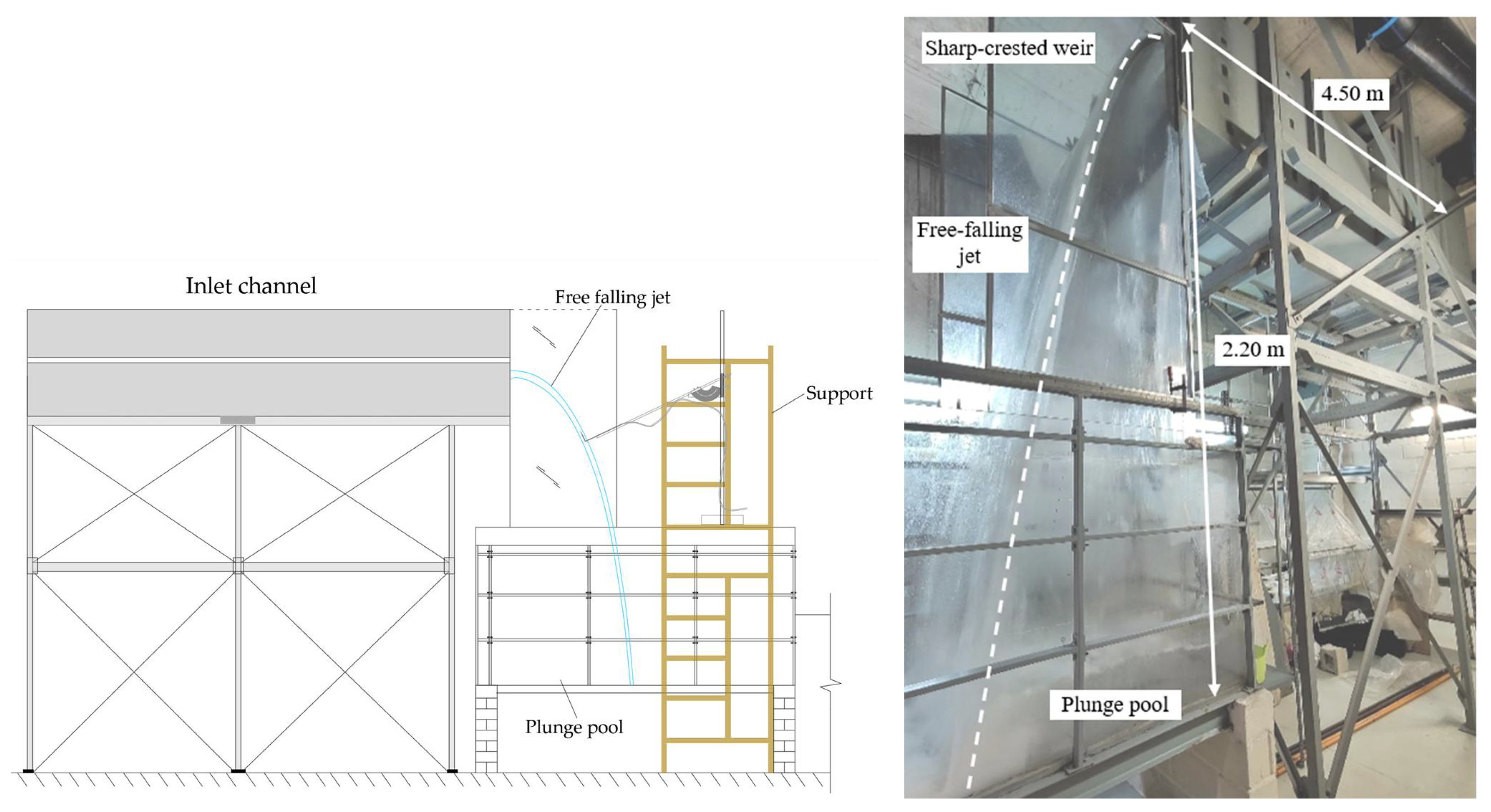
Measurements were obtained in a relatively large infrastructure (Figure 2) located at the Hydraulic Laboratory of the Universidad Politécnica de Cartagena (Spain). The inlet part consists of a mobile channel that is 4.50 m long and 1.05 m wide, with two gravels screens and a 0.30 m honeycomb wall to align the streamlines. The final part of the mobile device is a 1.50 m long channel that ends in a sharp-crested weir without lateral contractions. The sharp-crested weir has an elevation of 0.33 m from the bottom of the inlet channel and is located at an elevation of 2.20 m above the bottom of the stilling basin. The falling jet discharges into the atmosphere, and the upper and lower nappe side are in contact with open areas at atmospheric pressure, without any type of aeration restriction (see Figure 2).
3.2. Instrumentation
3.2.1. Conductivity Phase-Detection Probe
The air–water flow properties were analyzed using an intrusive conductivity phase-detection probe designed and built at the Universidad Politécnica de Cartagena (Carrillo et al. [7,8]). The design was based on other systems such as those used by Chanson [17,18,19], Matos et al. [20], and Felder and Chanson [3], among others. The platinum probe tip has a diameter Ø = 0.25 mm.
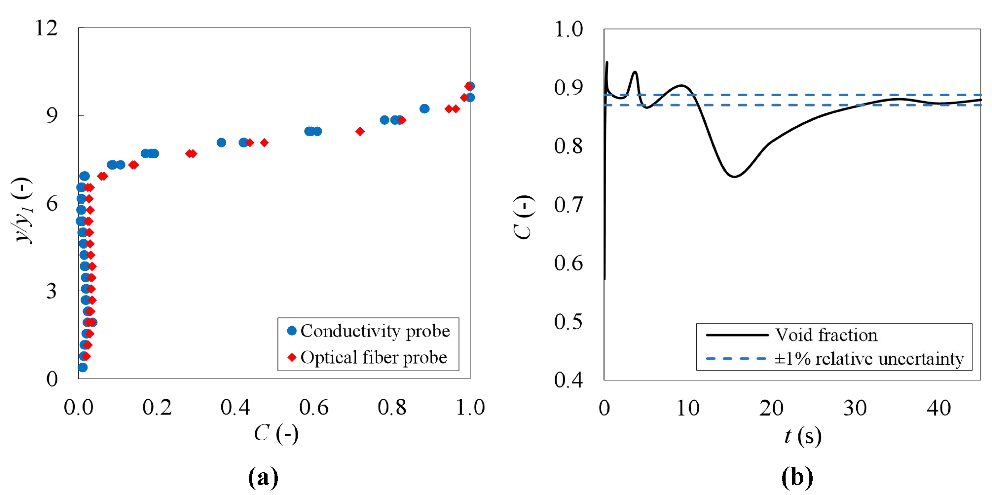
Ortega et al. [21] performed a comparison of the conductivity probe employed in this study with an RBI-Instrumentation optical fiber probe. The results showed maximum relative errors of the void fraction of below 5% in adverse conditions, such as a vertical profile in the center of the roller of a free hydraulic jump with supercritical Froude number Fr = 7.6, and flow depth upstream of the jump y1 = 0.013 m (Figure 3a). Those results are in agreement with the findings of Felder and Pfister [22], who obtained very close agreement between the two sensor types, namely with regard to the void fraction.
The phase-detection probe measures the changes in conductivity between the air and water phases by the different resistivity of the fluids. The raw signal is registered by the probe tip. A single-threshold method was used to convert the raw signal into a binary signal to identify the air and the water phases. The total time that the probe sensor tip is in air Σti over the total recorded time t is called the time-averaged void fraction (C = Σti/t). Figure 3b illustrates the evolution of the void fraction as the sampling time increases. According to our previous analyses, at least 30 s are needed in order to obtain a relative uncertainty of about ±1% in the local void fraction. Other authors such as Kramer et al. [23] suggest registers of at least 45 s to obtain accurate measurements. To err on the side of caution, in this study, each point was measured using a sampling rate of 20 kHz and a sampling duration of 45 s.
3.2.2. Back-Flushing Pitot Tube
The local velocity measurements were obtained with a modified Pitot-Prandtl tube, in which a back-flushing system avoids air entrainment in the pneumatic system (Matos and Frizell [24], Matos et al. [20]). The diameter hole of the dynamic pressure port was of 2.3 mm and the external diameter was 12 mm. The static pressure was measured by a ring of ports of 0.9 mm diameter placed in the body of the tube. The back-flushing system consists of a constant head reservoir that feeds the dynamic and the static pressure ports. To reduce the perturbation of the velocity measurements, the back-flushing flow rate was limited to near zero. The mean velocity was obtained considering Wood’s expression [25]:
where V is the local mean velocity, g is the gravitational acceleration, ΔP is the difference between the total pressure head and the static pressure head, ρw is the density of water, C is the local void fraction, and λ is the tapping coefficient, which accounts for the non-homogeneous behavior of the air–water flow near the stagnation point.
3.3. Experimental Tests and Flow Conditions
The origin of the coordinates was located in the weir crest, with X being the horizontal axis (positive to the downstream side) and Z the vertical axis (positive to the lower side; see Figure 1). Five different specific flow rates were tested for analyzing flow properties in nappe jets. The measurements were obtained in different cross-sections of the jet centerline located at different falling distances. The instrumentation was aligned with the main flow direction considering the theorical trajectory proposed by Scimemi [27]. The conductivity probe and the Pitot tube were displaced in the perpendicular direction of the jet centerline to measure the entire jet thickness with a spatial resolution of 1.0 mm. Cross-sections were measured from the weir crest to a maximum vertical falling distance of 2.0 m.
The test conditions and their non-dimensional numbers (Reynolds and Weber numbers, and , respectively, ρ being the density of fluid, Bi the jet thickness, µ the dynamic viscosity, and σ the surface tension) at the issuance conditions (at a vertical elevation Z = h from the weir crest) are summarized in Table 1. The jet break-up length Lb calculated with Equation (3) is also included. Considering the Scimemi [27] trajectory, the maximum measurable L/h ratio is also indicated, where L is the jet trajectory distance.
Experimental flow conditions were selected to avoid scale effects in the jet. According to several studies (e.g., Chanson [28], Heller [29]), when the total head in a sharp-crested weir is h > 0.045 m, the effects of scale may be neglected. However, for scaling air–water flows special caution must be taken, since some parameters, such as bubble chord sizes, cannot be correctly scaled (Chanson [28], Felder and Chanson [30]). Hence, the bubble mean diameter and the bubble chord length are very prone to scale effects. Some other parameters such as nappe oscillations cannot be scaled using Froude similitude as their characteristics seem to appear for the same unit discharge, independently of the weir size scale (Lodomez et al. [10])
4. Results and Discussion
4.1. Void Fraction Distributions
Air entrainment may affect the behavior of the rectangular jet and its free surface during the fall. Entrapped air changes the flow properties, such as the void fraction C and the jet thickness B. The water inner jet core evolution in two-phase jets has been analyzed by several authors (Chanson [31], Toombes and Chanson [32], Pfister and Schwindt [33]). However, studies that analyze the air–water properties in nappe jets remain scarce (Carrillo et al. [8]).
The local void fractions measurements were obtained with the conductivity phase-detection probe as the sum of the time the probe tip sensor was in the air ti over the total registered time t (C = Σti/t). The measurements were obtained in different cross-sections of the falling jets from 0.0 m to 2.0 m. A minimum of 30 points were measured per cross-section, so more than 3700 registers were obtained.
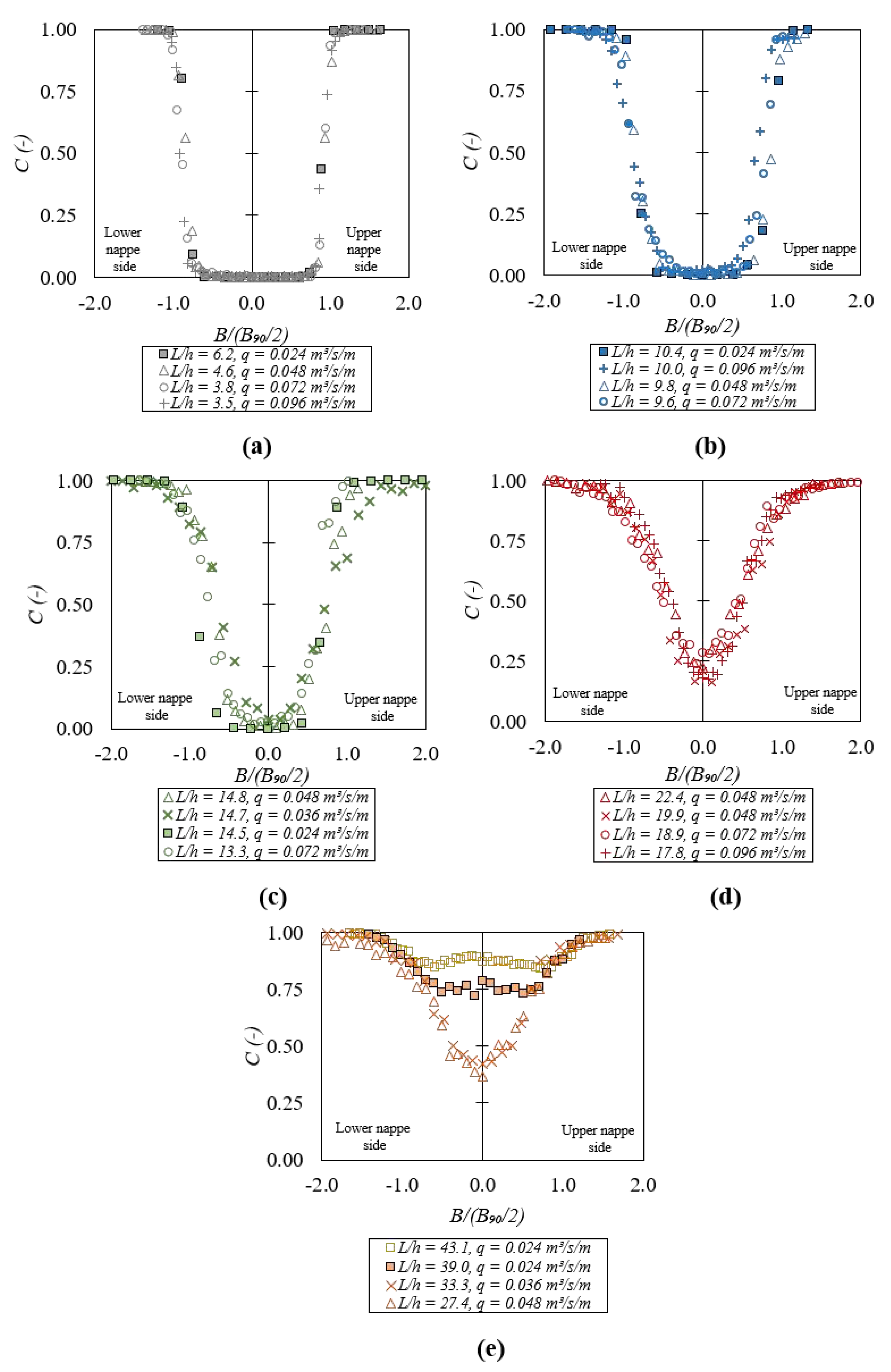
The B90 jet thickness was obtained as the distance in the perpendicular jet direction where the local void fraction C = 0.90, corresponding to the upper and lower nappe trajectories. The B90 values were used to obtain the center of each cross-section. The dimensionless parameter L/h was used to classify data in a non-dimensional way.
As the falling distance increases, the amount of air tends to increase, enlarging the width of the air–water mixing zone, and narrowing the non-aerated jet core. Figure 4 shows the void fraction distributions C as a function of the dimensionless jet thickness B/(B90/2). Data may be grouped as a function of the dimensionless falling distances L/h. For L/h ratios between 3.5 and 6.2 (Figure 4a) the void fraction profiles were similar, albeit with slight differences in the upper and lower nappe for the different specific flow rates. Those sections were also characterized by clear water conditions in the jet core (C = 0). In Figure 4b,c, the water jet core thickness tended to reduce as the flow fell due to the disturbances from free surfaces, with minor differences between the upper and lower nappe shapes. For L/h ratios between 17.8 and 22.4 (Figure 4d) it may be considered that the non-aerated water inner jet core has disappeared (minimum void fraction values between 0.13 < C < 0.28), and the slopes of the void fraction distribution were less steep than in the previous cases, which means that the air–water mixing zone tended to increase. For falling distances L/h larger than 27.4 (Figure 4e), the void fractions in the center of the jet tended to increase (from 0.37 to 0.89) depending on the L/h ratios. As the air entrainment increased, the slopes of the void fraction distributions tended to be less steep. It should be noted that those void fraction distributions may also consider the fluctuations observed in the surface of free-falling jets.
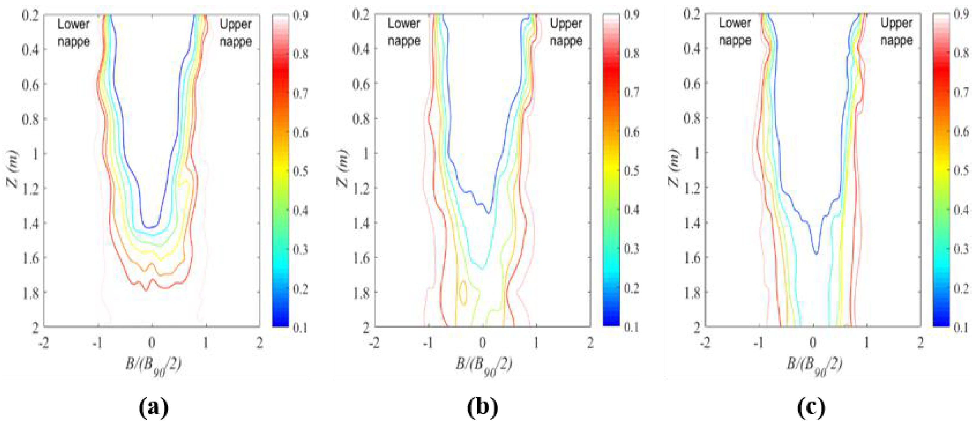
The contour maps plot in Figure 5 shows the void fraction evolution during the fall for three specific flow rates. The water inner core thickness decreased as the falling distance increased. Air was entraining at both sides of the jet, with no significant differences among the upper and the lower nappe trajectories. For the smaller and intermediate specific flow rates (0.024 and 0.048 m3/s/m) observed in Figure 5a,b, the non-aerated inner core with C = 0 disappeared when the falling distances Z ≥ 1.4–1.6. In the higher specific flow rate (Figure 5c), the non-aerated inner jet core tended to reach further distances during the measured falling distance of 2 m, with C ≈ 0.18 being its minimum void fraction in the further cross-section.
The mean void fraction Cmean of each cross-section is a characteristic parameter of the flow aeration that describes the thickness-averaged air content. It may be defined as:
where B is the jet thickness and C is the local void fraction.
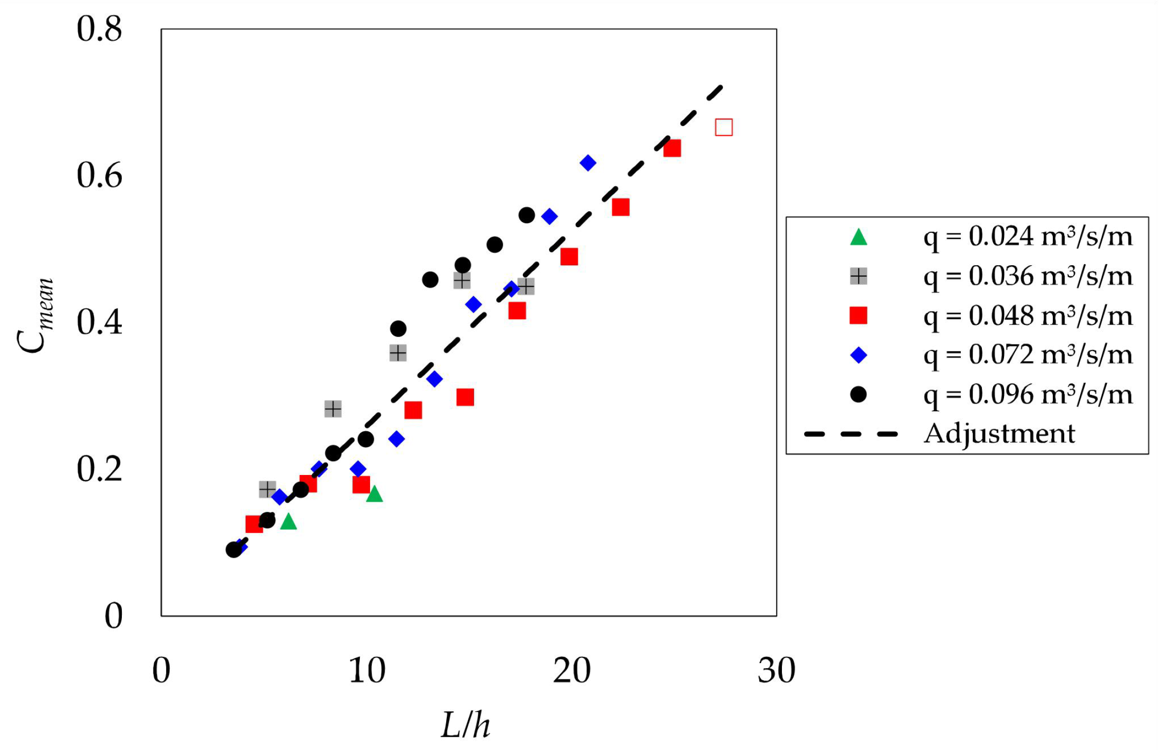
The mean void fraction evolution Cmean as a function of the dimensionless falling distance L/h is detailed in Figure 6. As the relative falling distance increased, the mean void fraction at the cross-sections tended to increase in a similar way for the different flow conditions: for falling distances L = 10h, Cmean ≈ 0.25; for falling distances L = 18h, Cmean ≈ 0.50. A potential behavior may be observed in the data (Cmean = 0.0246(L/h)1.0218), with R2 = 0.91. In the plot, data from the smaller specific flow rates with B50 < 0.7–0.8 mm were not considered because of a change in their trends, with B50 being the transversal distance between the upper and lower nappe trajectories with void fraction C = 0.50.
4.2. Jet Thickness and Spread
As was observed in the previous figures, the turbulence has a significant effect on the development of the jet surface disturbance and the spread of the jet thickness, with the inner jet core tending to reduce due to the growth of the air/water layer.
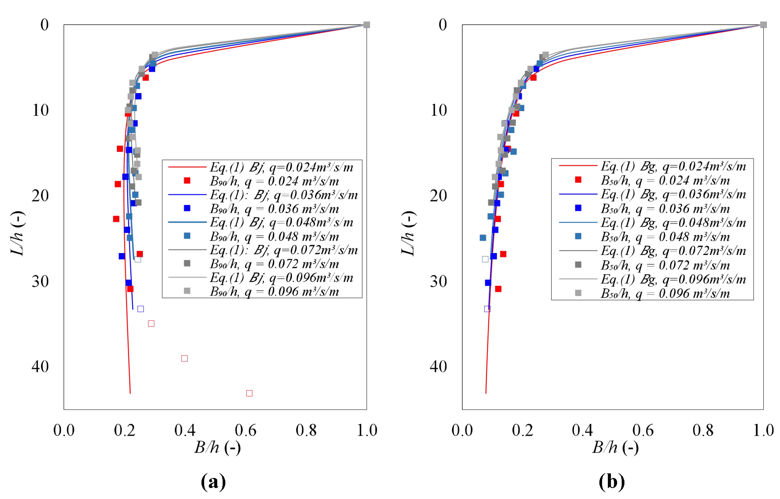
Figure 7a,b show the dimensionless evolution of the jet thicknesses B90 and B50, respectively. To facilitate the comparison, data were normalized as a function of the total energy head over the weir crest h. While the B50 values tended to reduce due to gravitational effects, the B90 values seemed to reach a constant value around 0.2h for non-dimensional falling distances between 10 < L/h < 30. For L/h > 33, there were no points with void fraction ≤0.5, making it impossible to calculate the B50 value. Beyond this point B90/h tended to increase rapidly; this may indicate that the break-up length was exceeded.
The experimental data were also compared with the jet thickness Bj calculated with Equation (1), and the theoretical jet thickness considering gravitational effects Bg. The B90 values seemed to be similar to the Bj values proposed by Castillo et al. [5], while the Bg was somewhat similar to the B50 measurements.
Considering B10 as the transversal thickness between the upper and lower nappe trajectories with void fraction C = 0.10, Figure 8 shows the slope in percentages that defines the inner core decay angle δ(B50–B10), the outer spread angle δ(B90–B50), and the total spread angle δ(B90–B10). Because of the reduced jet thickness of q = 0.024 m3/s/m (see Figure 5a), their B10 values were not considered in the plot. In general, the three lateral expansion angles seemed to be directly related with the jet velocity, increasing their values as the jet falls. Hence, the air–water mixing layer enlarged its thickness during the fall, generating the reduction of the non-aerated core and, at the same time, the increment of the lateral spread. The angles were similar to those reported by Ervine and Falvey [4] for circular falling jets.
Two adjustments were obtained for the outer spread angle δ(B90–B50) and the total spread angle δ(B90–B10), with R2 = 0.87 and 0.84, respectively.
where V is the mean velocity of the jet, and the angles are obtained as percentages.
4.3. Air–Water Phase Change
The phase-change count rate F is the number of air bubbles striking the probe tip per second. This statistical parameter may be considered a good estimator of the presence of air in two-phase flows (André et al. [34]).
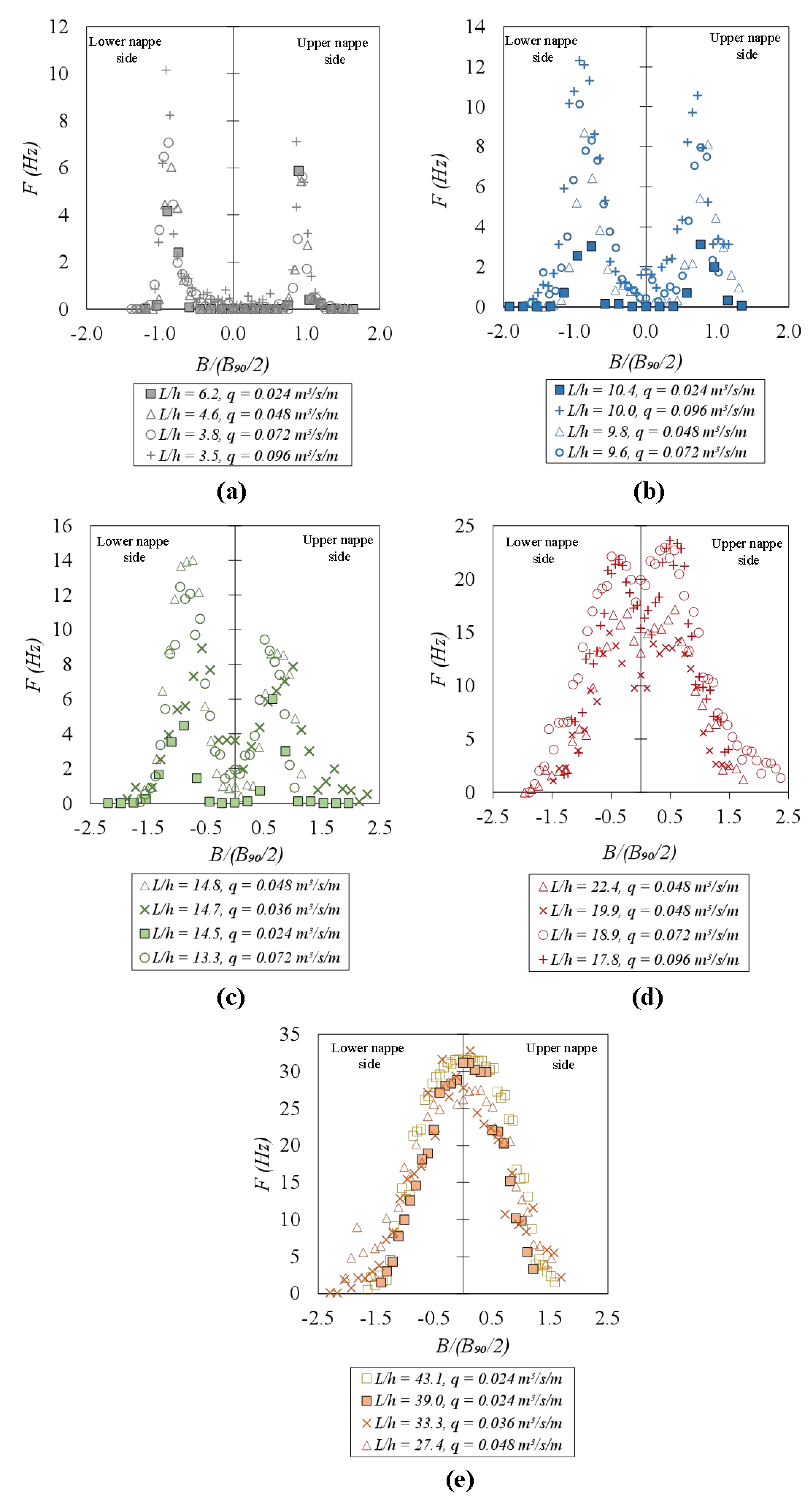
The phase-change count rate is presented in Figure 9 as a function of the dimensionless jet thickness B/(B90/2). As per the void fraction, data were classified as a function of the dimensionless falling distance L/h. For L/h ratios between 3.5 and 6.2 (Figure 9a), the maximum values were observed in the free surface of the jet, with some differences between the upper and lower nappe: maximum values between 6 and 10 Hz in the lower nappe side, and slightly smaller in the upper nappe side (between 3 and 8 Hz). In the center of the cross-sections, there was almost no air entrainment and frequencies were close to zero.
For dimensionless falling distances L/h of around 10 and 14 (Figure 9b,c) the maximum values were between 3 and 14 Hz in the lower nappe side, and between 3 and 11 Hz in the upper nappe side. The phase-change count rate remained between 2 and 4 Hz in the center of the cross-sections.
As the L/h ratio increased, and the jet cores aerated, the maximum values of phase-change count rate F increased and moved to the center of the jet. For L/h around 20 (Figure 9d), the non-aerated inner jet core disappeared, and the maximum frequency values tended to occur closer to the centerline. For L/h > 25 (Figure 9e), the maximum values were measured in the jet centerline, showing frequencies around 30 Hz.
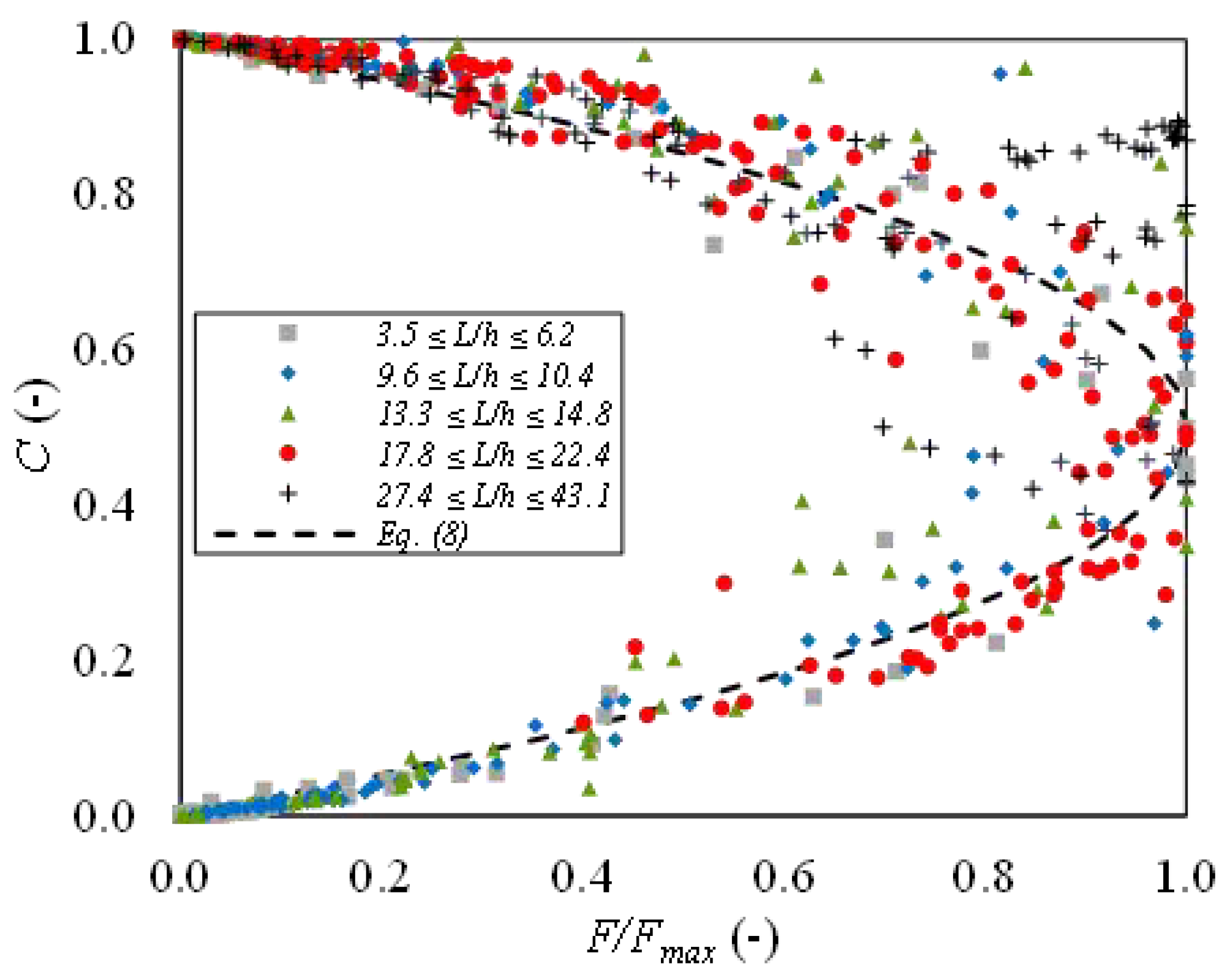
The maximum phase-change count rate in each cross-section Fmax is a further parameter for the quantification of the air entrainment performance (Felder and Chanson [35]). The relationship between the void fraction C and the dimensionless phase-change count rate F/Fmax was observed in several two-dimensional water jets and stepped cascades studies (e.g., Toombes [36], Brattberg et al. [37]). The data showed a self-similarity, and this relationship fits reasonably well with a parabolic shape:
With these considerations, the dimensionless air–water phase count rate is illustrated in Figure 10 as a function of the void fraction distribution. For the range of velocities tested (from 2.5 to 6.5 m/s), the air–water phase-change count rate showed its maximum values at about 50% of the local void fraction distribution (C ≈ 0.50). Considering the scattered data, the parabolic equations fit the experimental data in rectangular free-falling jets reasonably well, being independent of the jet velocity and the falling distance from the weir at the beginning of the fall. For dimensionless falling distances greater than L/h > 17.8, the values showed a different behavior due to the disappearance of the non-aerated inner core (see Figure 4).
4.4. Velocity Distributions
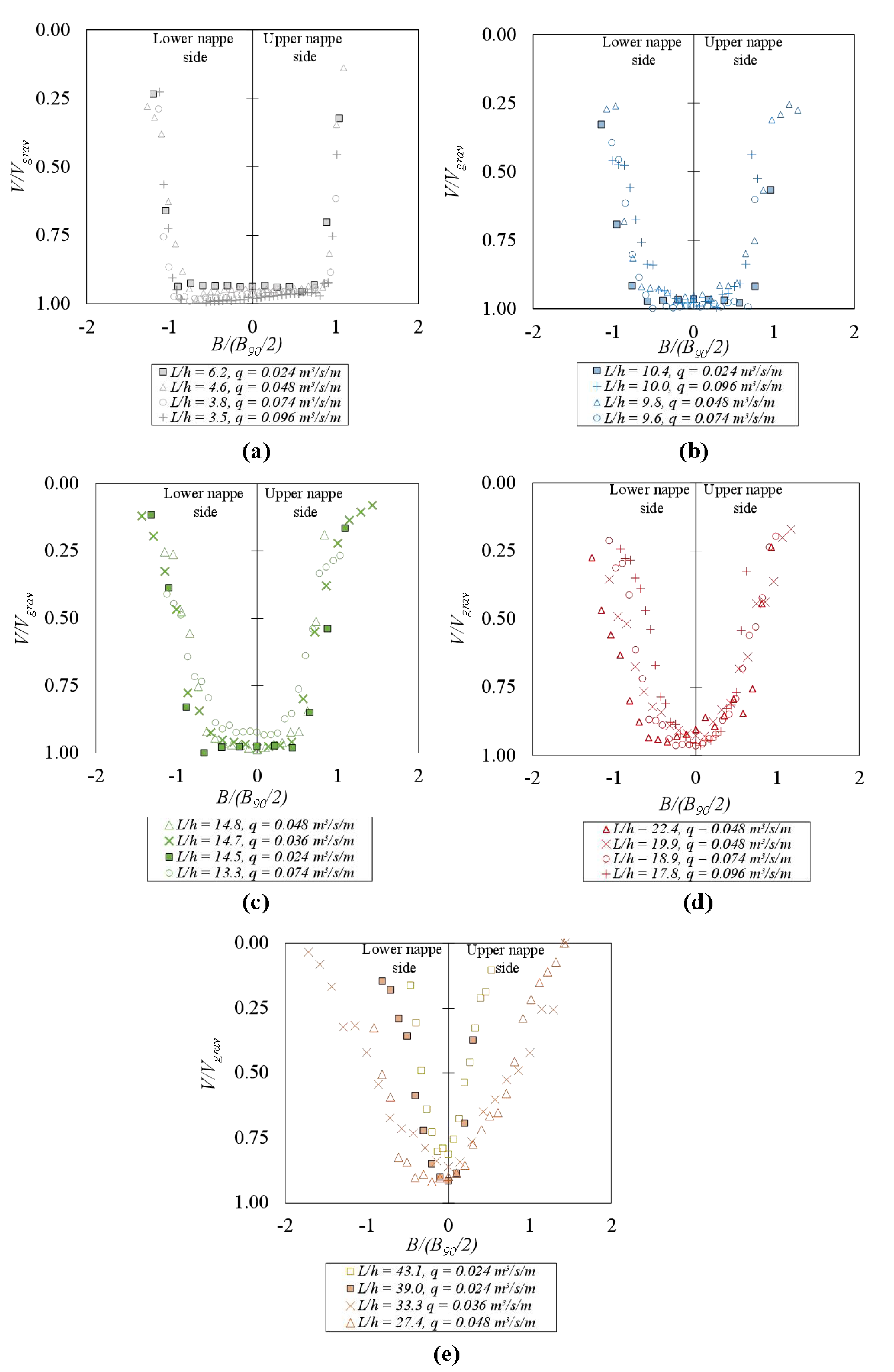
The local velocity data were obtained using a Pitot-Prandtl tube corrected by the local void fraction measured with the conductivity probe. Figure 10 shows the velocity profiles normalized as a function of the gravitational velocity in each cross-section (V/Vgrav), and the dimensionless jet thickness in different cross-sections considering the same grouping of the previous sections. The slopes of the cross-section profiles showed slight differences between the upper and lower nappe trajectories. The velocity increased along the falling jet in the central region of the cross-sections, due to gravitational acceleration. In all the cases, the maximum velocities were similar to their corresponding gravitational velocities. However, the velocity tended to reduce outside of the non-aerated core. Near the free surface the measurements with the Pitot-Prandtl tube should be considered with caution. The measurements may be less accurate due to the very high void fraction values. According to Matos et al. [20], the relative error of the velocity measurement increases significatively for high air concentrations (e.g., C > 0.9). In addition, it is not physically possible to obtain homogeneous air–water mixtures for C > 0.75, as mentioned in Matos [38], and Equation (4) may be less accurate.
For dimensionless falling distances L/h ratios between 3.5 and 6.2 (Figure 11a), there was a slight change of slope between the transition of the upper and lower interfaces due to the surface curvature of nappe flows. For values between 9.6 < L/h < 22.4 (Figure 11b–d) the reduction of the non-aerated inner jet core seemed to be related to the deceleration outside of the central part of the velocity profile, reducing the differences between the shape reordered in the upper and lower nappe trajectories. For L/h > 33.3 (Figure 11e), the central part of the velocity profile disappeared and the velocity distribution was sharper. The maximum mean velocity tended to decrease slightly due to the high air entrainment.
4.5. Energy Dissipation
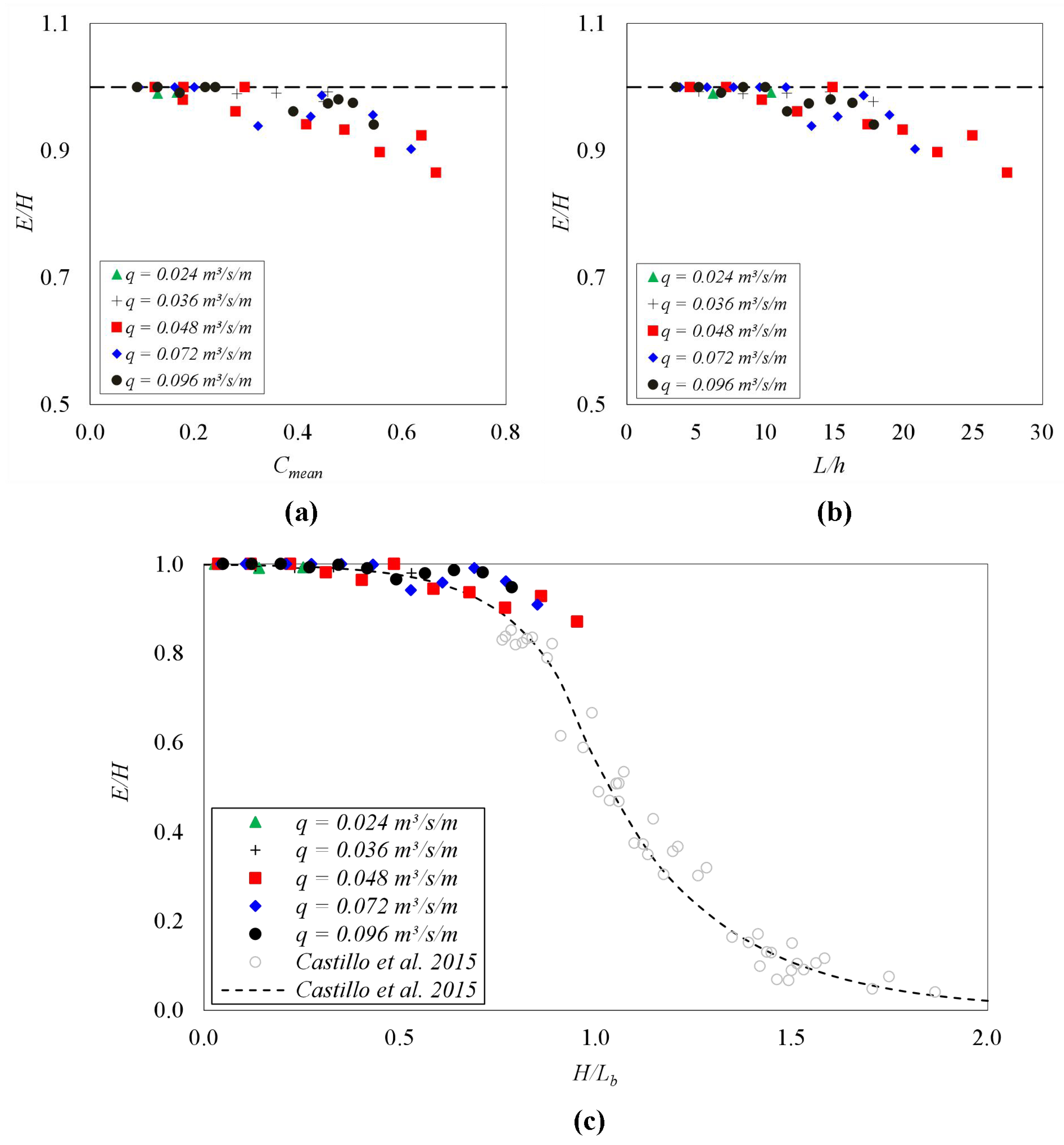
Considering the parameters measured in the previous sections (see for instance Figure 6), the development of the jet energy E during the fall may be analyzed as a function of the vertical distance between the total energy line and the analyzed cross-section H (see Figure 1). Figure 12a shows the dimensionless energy E/H as a function of Cmean. For mean void fractions <0.2–0.3 the energy of the jet seemed to be constant, since the amount of air entrapped in the jet was limited and the water jet core was not significantly affected. However, as the mean void fraction increased, the energy of the jet began to be dissipated. For Cmean values larger than 0.4–0.5, the energy dissipation tended to increase rapidly, with an evident change in the slope of the plot.
A similar study may be considered as a function of the non-dimensional falling distance L/h ratio (Figure 12b). For L/h ratio < 10–15, there was no notable reduction in the total energy of the jet. However, for larger falling distances the energy dissipation tended to increase. For falling distance ratios larger than 15, all data showed a clear energy dissipation, increasing as the L/h ratio increased.
Carrillo [13] and Castillo et al. [5] studied the dimensionless energy of rectangular free-falling jets analyzing instantaneous pressures measured at the bottom of the plunge pool. Employing an inverse methodology from their pressure measurements with non-effective water cushions, the authors obtained an adjustment of the dimensionless energy as a function of the H/Lb ratio (if H/Lb < 1.00, ; if H/Lb ≥ 1.00, ). Following this dimensionless falling distance, Figure 12c compares the data obtained in this study with the adjustment obtained by Castillo et al. [5] and their experimental data. Although the experimental methodology and the registered variables in both studies are different, generally speaking, the values obtained follow the behavior previously reported by the authors. The main differences were found for H/Lb ≈ 0.7–1.0, where both experimental campaigns overlapped. This region corresponded to falling distances near the break-up length, with a sudden change in the energy dissipation behavior. In addition, we noticed that in the experiments analyzed by Castillo et al. [5], there was always a water cushion behind the falling jet. The presence of the water cushion and the mixing process in the pool are thus expected to increase the energy dissipation measured in the stagnation point, generating an additional energy loss with respect to the current experimental campaign.
4.6. Sauter Mean Bubble Diameter
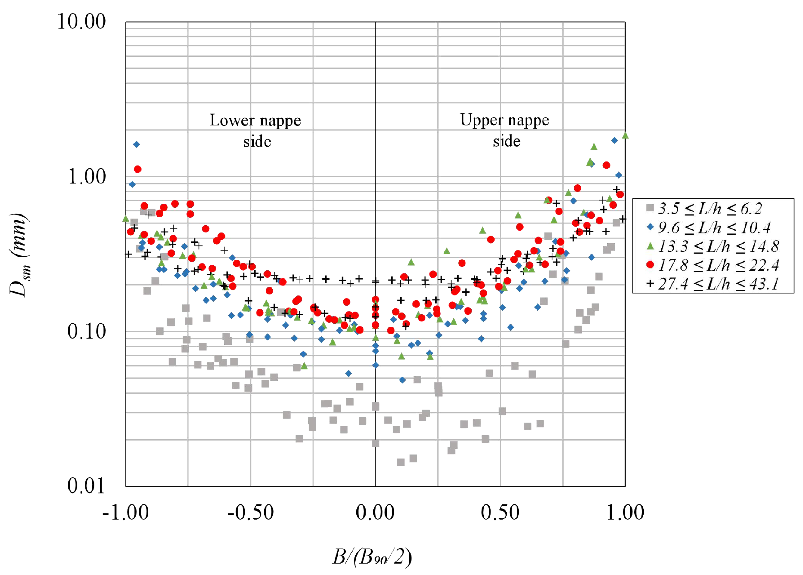
If phase changes detected by the conductivity probe are simplified to be considered spherical in shape and equally distributed, the Sauter mean bubble diameter Dsm (Clift et al. [39]) may be obtained. The Dsm is defined as:
where C is the local void fraction, V is the local mean velocity obtained with Equation (4) assuming the air bubbles have the same velocity as the flow, and F is the phase-change count rate.
Figure 13 shows the Sauter mean bubble diameter calculated at different falling distances from the weir. As in the previous figures, the values plotted were limited to C ≤ 0.90 values. The Dsm values were mostly between 0.1 and 1.0 mm, with maximum values below 3.0 mm. The minimum values are registered in the center of the jet, whilst the maximum values are near the free surface. In the center of the jet, smaller values of the Sauter mean bubble diameter were obtained for cross-sections located at relative falling distances between 3.5 and 6.2. Those diameter values may be related to the difficulty in measuring with the phase-detection probe at points with relatively small frequency detection F and air content C. Once the air enters the jet, the Dsm distribution in the cross-sections seems to be relatively independent of the specific flow rate. The upper and lower nappe sides showed near a symmetrical behavior. The skewness values calculated per specific flow rate were between 1 and 3, indicating that there was a low asymmetry of the mean bubble diameter to the upper nappe side.
4.7. Air–Water Chord Length
The air–water chord length distribution Ch represents the variation in chord length sizes of air bubbles or water droplets (Toombes [36]). The chord length may be used as a characteristic indicator for the air–water interfaces (Felder and Chanson [35]). The bubble chord length can be calculated as:
where V is the local mean velocity obtained with Equation (4), and tch is the chord time defined as the time spent by the air/water interface on the probe tip.
The chord-length distribution of air–water flows may be represented by a probability density function (PDF) in the form of a frequency histogram (e.g., Toombes [36], Chanson and Carosi [40], Felder [41]). Figure 14 shows the comparison of the probability density distribution calculated for the chord length in three different points of the upper nappe trajectory with C ≈ 0.90. The compared points were located at different non-dimensional falling distances, with local velocities between 3.5 and 5.7 m/s. In general, the highest values of the probability distribution function were located for chord length scales between 0 and 2 mm. As the velocity of the falling jet V and the dimensionless falling distances L/h increased, the PDF values decreased rapidly.
These data agree with the results obtained by Brattberg et al. [37] in two-dimensional water jets, whose higher probabilities were found between 0.5 and 2.0 mm, along with maximum bubble chord lengths of up to 100 mm.
5. Conclusions
The aeration processes in rectangular free-falling jets are due to instabilities and turbulent fluctuations close to the air–water free-surface that act on the upper and lower nappe sides of the jets during the fall. Self-aeration processes change the flow properties and affect the non-aerated inner core of the jet.
At the beginning of the falling distance, the void fraction distributions in the cross-sections of the jets showed that the non-aerated inner core (C = 0) requires a trajectory distance L larger than 15 times the total energy head over the weir crest to be affected. As the falling distance increases, the non-aerated inner jet core tends to disappear by air entrainment processes. Hence, for dimensionless falling distances L/h > 17.8, the jet core presented void fraction values larger than 0.1; for L/h > 27.4, the void fraction in the entire cross-section exceeded 0.37.
The parametric methodology proposed by Castillo et al. [5] seemed to follow the jet thickness with C = 0.90. Moreover, the thickness corresponding to C = 0.50 agreed with the gravitational thickness. The lateral expansion angles were in agreement with those reported by Ervine and Falvey [4] for circular jets.
Near the weir crest (L/h < 15–20), the relationship between the bubble frequency and the void fraction seemed to have a good fit with the parabolic behavior reported by Toombes [35] and Brattberg et al. [36] in other kinds of air–water flows. The maximum values of F/Fmax were obtained around C = 0.40 and 0.60 in the majority of the cross-sections analyzed.
The energy of the jet seemed to be conserved until the mean void fraction of the cross-section was 0.2–0.3. However, as the mean void fraction increased, the energy dissipation also increased. Similar behavior may also be observed for L/h > 15. Although the obtained data show relatively good agreement with previous published trends in the dimensionless energy as a function of the H/Lb ratio, this region near the break-up length requires further analysis to improve the current knowledge of its energy dissipation.
The Sauter mean diameter distribution showed slight differences between the upper and lower nappe sides. Once the relative falling distance was larger than 10, the mean diameter distribution seemed to show the same behavior, independently of the specific flow rate and the falling distance.
Although the experimental facility enables us to analyze the flow with the recommendations to avoid scale effects and systematic errors in the measurements, the air–water flow characteristics may not be exempt from scale effects. Those effects would lead us to err on the side of caution if data were extrapolated to larger Froude scale models.
In some analysis (Figure 8), the data of the smaller specific flow rate (0.024 m3/s/m) did not follow the general trend observed in the other cases. Although the sharp weir crest used in this study was different from those analyzed by Anderson and Tullis [9] and Lodomez et al. [10] (who analyzed round crest weirs), the nappe oscillation phenomenon may have appeared in the smaller head condition of this study. Additional studies are needed to better understand the detailed effect of the energy head and the crest profile on the flow characteristics.
Author Contributions
Conceptualization, J.M.C.; Data curation, P.R.O.; Formal analysis, J.M.C., P.R.O. and J.T.G.; Funding acquisition, J.M.C. and L.G.C.; Investigation, P.R.O.; Methodology, J.M.C.; Project administration, J.M.C. and L.G.C.; Resources, J.M.C. and L.G.C.; Validation, J.M.C., P.R.O., L.G.C., and J.T.G.; Visualization, P.R.O.; Writing–original draft, J.M.C. and P.R.O.; Writing–review and editing, J.M.C., P.R.O., L.G.C., and J.T.G. All authors have read and agreed to the published version of the manuscript.
Funding
This research was funded by the “Ministerio de Ciencia, Innovación y Universidades” (MCIU), the “Agencia Estatal de Investigación” (AEI) and the “Fondo Europeo de Desarrollo Regional” (FEDER), through the Project “La aireación del flujo en el vertido en lámina libre por coronación de presas a nivel de prototipo y su efecto en cuencos de disipación de energía”, grant number: RTI2018-095199-B-I00, and by the “Comunidad Autónoma de la Región de Murcia” for the financial aid received through the “Programa Regional de Fomento de la Investigación Científica y Técnica (Plan de Actuación 2018) de la Fundación Séneca-Agencia de Ciencia y Tecnología de la Región de Murcia”, Project “Análisis de la capacidad de descarga de vertederos tipo laberinto y de la disipación de energía aguas abajo de los mismos”, grant number: 20879/PI/18.
Institutional Review Board Statement
Not applicable.
Informed Consent Statement
Not applicable.
Data Availability Statement
Some or all data, models, or code that support the findings of this study are available from the corresponding author upon reasonable request.
Conflicts of Interest
The authors declare that they have no known competing financial interests or personal relationships that could have appeared to influence the work reported in this paper.
Notations
The following symbols are used in this paper:
| B | jet thickness in the analyzed cross-section |
| Bg | jet thickness due to gravitational effects |
| Bi | jet thickness at the issuance conditions |
| Bj | jet thickness |
| B90 | jet thickness with void fraction C |
| B50 | jet thickness with void fraction C |
| B10 | jet thickness with void fraction C |
| C | local void fraction |
| Cd | discharge coefficient for sharp weir crest |
| Ch | bubble chord length |
| Cmean | mean void fraction |
| Dsm | Sauter mean diameter |
| E | energy at the analyzed cross-section |
| F | air–water phase count rate |
| Fi | Froude number at the issuance conditions |
| Fmax | maximum air–water phase count rate |
| Fr | Froude number |
| g | gravitational acceleration |
| h | total energy head over the weir crest |
| H | vertical distance between the reference level of the total energy line and the analyzed cross-section |
| IC | initial conditions |
| K | non-dimensional coefficient |
| Kφ | experimental term of the turbulence parameter φ |
| L | jet trajectory distance |
| Lb | jet break-up length |
| probability density function | |
| q | specific flow rate or water discharge per unit width |
| Re | Reynolds number |
| Tu | turbulent intensity at the issuance conditions |
| Tu* | turbulence intensity |
| t | time-averaged void fraction |
| tch | chord time |
| V | local mean velocity |
| Vgrav | gravitational velocity |
| root-mean-square of the velocity fluctuation | |
| Vi | mean velocity at the issuance conditions |
| We | Weber number |
| X | horizontal axis |
| Z | vertical axis |
| ΔP | difference between the total pressure head and the static pressure head |
| Σti | total recorded time |
| δ | spread angle |
| ξ | lateral spread |
| λ | tapping coefficient for the non-homogeneous behavior of the air–water flow |
| ν | kinematic viscosity |
| µ | dynamic viscosity |
| ρ | density of fluid |
| ρw | density of water |
| σ | surface tension |
| Ø | probe diameter and |
| φ | turbulence parameter in nappe flow. |
References
- Federal Emergency Management Agency. FEMA. P-1015 Technical Manual: Overtopping Protection for Dams; US Department of Homeland Security: Denver, CO, USA, 2014. Available online: https://www.fema.gov/es/media-library/assets/documents/97888 (accessed on 15 March 2021).
- Wahl, T.L.; Frizell, K.H.; Cohen, E.A. Computing the trajectory of free jets. J. Hydraul. Eng. 2008, 134, 256–260. [Google Scholar] [CrossRef] [Green Version]
- Felder, S.; Chanson, H. Phase-detection probe measurements in high-velocity free-surface flows including a discussion of key sampling parameters. Exp. Therm. Fluid Sci. 2014, 61, 66–78. [Google Scholar] [CrossRef]
- Ervine, D.A.; Falvey, H. Behaviour of turbulent jets in the atmosphere and plunge pools. P. I. Civil Eng. 1987, 83, 295–314. [Google Scholar] [CrossRef]
- Castillo, L.; Carrillo, J.M.; Blázquez, A. Plunge pool mean dynamic pressures: A temporal analysis in nappe flow case. J. Hydraul. Res. 2015, 53, 101–118. [Google Scholar] [CrossRef]
- Bertola, N.; Wang, H.; Chanson, H. A physical study of air-water flow in planar plunging water jet with large inflow distance. Int. J. Multiph. Flow 2017, 100, 155–171. [Google Scholar] [CrossRef] [Green Version]
- Carrillo, J.M.; Ortega, P.R.; Castillo, L.G.; García, J.T. Air entrainment in rectangular free falling jets. In Proceedings of the 8th IAHR Int. Symp. on Hydraulic Structures, Santiago, Chile, 12–15 May 2020. [Google Scholar] [CrossRef]
- Carrillo, J.M.; Ortega, P.R.; Castillo, L.G.; García, J.T. Experimental Characterization of Air Entrainment in Rectangular Free Falling Jets. Water 2020, 12, 1773. [Google Scholar] [CrossRef]
- Anderson, A.A.; Tullis, B.P. Finite crest length weir nappe oscillation. J. Hydraul. Eng. 2018, 144, 04018020. [Google Scholar] [CrossRef]
- Lodomez, M.; Tullis, B.; Dewals, B.; Archambeau, P.; Kitsikoudis, V.; Pirotton, M.; Erpicum, S. Nappe oscillations on free-overfall structures: Size scale effects. J. Hydraul. Eng. 2019, 145, 04018022. [Google Scholar]
- Horeni, P. Disintegration of a Free Jet of Water in Air; Byzkumny ustav vodohospodarsky prace a studie; VÝCHODOĆESKÉ MUZEUM V PARDUBICÍCH: Praha, Czech Republic, 1956. (In Czech) [Google Scholar]
- Castillo, L. Aerated jets and pressure fluctuation in plunge pools. In Proceedings of the Seventh International Conference on Hydroscience and Engineering, M. Piasecki and College of Engineering, Drexel University, Philadelphia, PA, USA, 10–13 September 2006; pp. 1–23. [Google Scholar]
- Carrillo, J.M. Metodología Numérica y Experimental Para el Diseño de los Cuencos de Disipación en el Sobrevertido de Presas de Fábrica. PhD Thesis, Universidad Politécnica de Cartagena, Cartagena, Spain, 2014. Available online: https://repositorio.upct.es/handle/10317/4038 (accessed on 10 June 2014). (In Spanish).
- Castillo, L.G.; Carrillo, J.M.; Sordo-Ward, A. Simulation of overflow nappe impingement jets. J. Hydroinform. 2014, 16, 922–940. [Google Scholar] [CrossRef] [Green Version]
- Carrillo, J.M.; Castillo, L.G.; Marco, F.; García, J.T. Experimental and numerical analysis of two-phase flows in plunge pools. J. Hydraul. Eng. 2020, 146, 04020044. [Google Scholar] [CrossRef] [Green Version]
- Carrillo, J.M.; Marco, F.; Castillo, L.G.; García, J.T. Experimental study of submerged hydraulic jumps generated downstream of rectangular plunging jets. Int. J. Multiph. Flow 2021, 137, 103579. [Google Scholar] [CrossRef]
- Chanson, H. Air Bubble Entrainment in Free-Surface Turbulent Shear Flows, 1st ed.; Academic Press: London, UK, 1997. [Google Scholar]
- Chanson, H. Air bubble entrainment in open channels. Flow structure and bubble size distributions. Int. J. Multiph. Flow 1997, 23, 193–203. [Google Scholar] [CrossRef] [Green Version]
- Chanson, H. Air-water Flows in Water Engineering and Hydraulic Structures. Basic Processes and Metrology. In Proceedings of the Hydraulics of Dams and River Structures; Yazdandoost, F., Attari, J., Eds.; CRC Press: London, UK, 2004; p. 50. [Google Scholar]
- Matos, J.; Frizell, K.H.; André, S.; Frizell, K.W. On the performance of velocity measurement techniques in air-water flows. In Hydraulic Measurements and Experimental Methods; ASCE: Minneapolis, MN, USA, 2002; pp. 130–140. [Google Scholar]
- Ortega, P.R.; Carrillo, J.M.; Castillo, L.G.; García, J.T. Análisis experimental de flujos bifásicos en resaltos hidráulicos. In Proceedings of the Jornadas de Ingeniería del Agua, Toledo, Spain, 23–24 October 2019. (In Spanish). [Google Scholar]
- Felder, S.; Pfister, M. Comparative analysis of phase-detective intrusive probes in high-velocity air-water flows. Int. J. Multiph. Flow 2017, 90, 88–101. [Google Scholar] [CrossRef] [Green Version]
- Kramer, M.; Hohermuth, B.; Valero, D.; Felder, S. Best practices for velocity estimations in highly aerated flows with dual-tip phase-detection probes. Int. J. Multiph. Flow 2020, 126, 103228. [Google Scholar] [CrossRef] [Green Version]
- Matos, J.; Frizell, K.H. Air concentration and velocity measurements on self-aerated flow down stepped chutes. In Proceedings of the Joint Conf. on Water Resources Engineering and Water Resources Planning & Management, ASCE, Minneapolis, MN, USA, 30 July–2 August 2000. [Google Scholar]
- Wood, I.R. Uniform region of self-aerated flow. J. Hydraul. Div. ASCE 1983, 109, 447–461. [Google Scholar] [CrossRef]
- Chamani, M.R.; Rajaratnam, N. Characteristics of skimming flow over stepped spillways. J. Hydraul. Eng. 1999, 105, 361–368. [Google Scholar] [CrossRef]
- Scimemi, E. Sulla forma delle vene tracimanti. L’Energia Elettr. 1931, 7, 293–305. (In Italian) [Google Scholar]
- Chanson, H. Turbulent air-water flows in hydraulic structures: Dynamic similarity and scale effects. Environ. Fluid Mech 2009, 9, 125–142. [Google Scholar] [CrossRef] [Green Version]
- Heller, V. Scale effects in physical hydraulic engineering models. J. Hydraul. Res. 2011, 49, 293–306. [Google Scholar] [CrossRef]
- Felder, S.; Chanson, H. Scale effects in microscopic air-water flow properties in high-velocity free-surface flows. Exp. Therm. Fluid Sci. 2016, 83, 19–36. [Google Scholar] [CrossRef] [Green Version]
- Chanson, H. Velocity measurements within high velocity air-water jets. J. Hydraul. Res. 1993, 31, 365–382. [Google Scholar] [CrossRef] [Green Version]
- Toombes, L.; Chanson, H. Free-surface aeration and momentum exchange at a bottom outlet. J. Hydraul. Res. 2007, 45, 100–110. [Google Scholar] [CrossRef]
- Pfister, M.; Schwindt, S. Air concentration distribution in deflector jets. In Proceedings of the 5th IAHR International Symposium on Hydraulic Structures, Brisbane, Australia, 25–27 June 2014. [Google Scholar]
- André, S.; Boillat, J.L.; Schleiss, A.J. Two-phase flow characteristics of stepped spillways’. J. Hydraul. Eng. 2005, 131, 423–427. [Google Scholar] [CrossRef]
- Felder, S.; Chanson, H. Aeration and Air–Water Mass Transfer on Stepped Chutes with Embankment Dam Slopes. Environ. Fluid Mech. 2015, 15, 695–710. [Google Scholar] [CrossRef] [Green Version]
- Toombes, L. Experimental Study of Air-Water Flow Properties on Low-Gradient Stepped Cascades. Ph.D. Thesis, School of Civil Engineering, The University of Queensland, Brisbane, Australia, 2002. Available online: https://espace.library.uq.edu.au/view/UQ:9270 (accessed on 20 July 2020).
- Brattberg, T.; Toombes, L.; Chanson, H. Developing air-water shear layers of two-dimensional water jets discharging into air. In Proceedings of the ASME Fluids Engineering Division Summer Meeting (FEDSM’98), Washington, DC, USA, 21–25 June 1998. [Google Scholar]
- Matos, J. Discussion of the “Characteristics of skimming flow over stepped spillways”. J. Hydraul. Eng. 2000, 126, 865–869. [Google Scholar] [CrossRef]
- Clift, R.; Grace, J.R.; Weber, M.E. Bubbles, Drops and Particles; Academic Press: New York, NY, USA, 1978; p. 380. [Google Scholar]
- Chanson, H.; Carosi, G. Advanced post-processing and correlation analyses in high-velocity air-water flows. Environ. Fluid Mech 2007, 7, 495–508. [Google Scholar] [CrossRef] [Green Version]
- Felder, S. Air-Water Flow Properties on Stepped Spillways for Embankment Dams: Aeration, Energy Dissipation and Turbulence On Uniform, Non-Uniform and Pooled Stepped Chutes. Ph.D. Thesis, School of Civil Engineering, The University of Queensland, Brisbane, Australia, 2013. Available online: https://espace.library.uq.edu.au/view/UQ:301329 (accessed on 11 May 2019).
Figure 1.
Representation of a rectangular free-falling jet spreading in the atmosphere.

Figure 2.
Experimental device of rectangular free-falling jet.

Figure 3.
Analysis of the conductivity probe: (a) comparison with an optical fiber probe in the center of the roller of a hydraulic jump with Fr = 7.6 (adapted from Ortega et al. [21]); (b) evolution of the void fraction during a sampling test.
Figure 3.
Analysis of the conductivity probe: (a) comparison with an optical fiber probe in the center of the roller of a hydraulic jump with Fr = 7.6 (adapted from Ortega et al. [21]); (b) evolution of the void fraction during a sampling test.

Figure 4.
Void fraction distributions as a function of the dimensionless jet thickness B/(B90/2): (a) L/h ratio between 3.5 and 6.2; (b) L/h ratio between 9.6 and 10.4; (c) L/h ratio between 13.3 and 14.8; (d) L/h ratio between 17.8 and 22.4; (e) L/h ratio between 27.4 and 43.1.
Figure 4.
Void fraction distributions as a function of the dimensionless jet thickness B/(B90/2): (a) L/h ratio between 3.5 and 6.2; (b) L/h ratio between 9.6 and 10.4; (c) L/h ratio between 13.3 and 14.8; (d) L/h ratio between 17.8 and 22.4; (e) L/h ratio between 27.4 and 43.1.

Figure 5.
Contour map of void fraction distributions C as a function of the dimensionless thickness B/(B90/2): (a) q = 0.024 m3/s/m; (b) q = 0.048 m3/s/m; (c) q = 0.096 m3/s/m.
Figure 5.
Contour map of void fraction distributions C as a function of the dimensionless thickness B/(B90/2): (a) q = 0.024 m3/s/m; (b) q = 0.048 m3/s/m; (c) q = 0.096 m3/s/m.

Figure 6.
Mean void fraction as a function of dimensionless falling distance L/h (filled marker: case L ≤ Lb; unfilled marker: case L > Lb).
Figure 6.
Mean void fraction as a function of dimensionless falling distance L/h (filled marker: case L ≤ Lb; unfilled marker: case L > Lb).

Figure 7.
Evolution of the dimensionless jet thickness during the fall (filled marker: case L ≤ Lb; unfilled marker: case L > Lb): (a) B90/h and Bj/h; (b) B50/h and Bg/h.
Figure 7.
Evolution of the dimensionless jet thickness during the fall (filled marker: case L ≤ Lb; unfilled marker: case L > Lb): (a) B90/h and Bj/h; (b) B50/h and Bg/h.

Figure 8.
Lateral expansion angles as a function of the jet velocity.

Figure 9.
Air–water phase-change count rate as a function of dimensionless jet thickness B/(B90/2): (a) L/h ratio between 3.5 and 6.2; (b) L/h ratio between 9.6 and 10.4; (c) L/h ratio between 13.3 and 14.8; (d) L/h ratio between 17.8 and 22.4; (e) L/h ratio between 27.4 and 43.1.
Figure 9.
Air–water phase-change count rate as a function of dimensionless jet thickness B/(B90/2): (a) L/h ratio between 3.5 and 6.2; (b) L/h ratio between 9.6 and 10.4; (c) L/h ratio between 13.3 and 14.8; (d) L/h ratio between 17.8 and 22.4; (e) L/h ratio between 27.4 and 43.1.

Figure 10.
Dimensionless air–water phase-change count rate F/Fmax as a function of the void fraction distribution C.
Figure 10.
Dimensionless air–water phase-change count rate F/Fmax as a function of the void fraction distribution C.

Figure 11.
Dimensionless velocity distribution V/Vmax through the rectangular free-falling jet: (a) L/h ratio between 3.5 and 6.2; (b) L/h ratio between 9.6 and 10.4; (c) L/h ratio between 13.3 and 14.8; (d) L/h ratio between 17.8 and 22.4; (e) L/h ratio between 27.4 and 43.1.
Figure 11.
Dimensionless velocity distribution V/Vmax through the rectangular free-falling jet: (a) L/h ratio between 3.5 and 6.2; (b) L/h ratio between 9.6 and 10.4; (c) L/h ratio between 13.3 and 14.8; (d) L/h ratio between 17.8 and 22.4; (e) L/h ratio between 27.4 and 43.1.

Figure 12.
Dimensionless energy E/H: (a) as a function of Cmean; (b) as a function of the L/h ratio; (c) as a function of the H/Lb ratio.
Figure 12.
Dimensionless energy E/H: (a) as a function of Cmean; (b) as a function of the L/h ratio; (c) as a function of the H/Lb ratio.

Figure 13.
Sauter mean bubble diameter in rectangular free-falling jets as a function of the dimensionless jet thickness.
Figure 13.
Sauter mean bubble diameter in rectangular free-falling jets as a function of the dimensionless jet thickness.

Figure 14.
Probability density function of air bubble chord lengths in rectangular jets.


Table 1.
Characteristics of the tests at the issuance conditions.
| q (m3/s/m) | h (m) | Vi (m/s) | Re (-) | We (-) | Lb (m) | Maximum L (m) | Maximum L/h(-) |
|---|---|---|---|---|---|---|---|
| 0.024 | 0.050 | 1.40 | 24,021 | 464 | 1.78 | 2.13 | 43.1 |
| 0.036 | 0.065 | 1.60 | 35,561 | 789 | 2.01 | 2.17 | 33.3 |
| 0.048 | 0.080 | 1.78 | 47,148 | 1162 | 2.19 | 2.21 | 27.4 |
| 0.072 | 0.109 | 2.07 | 70,721 | 2029 | 2.48 | 2.27 | 20.8 |
| 0.096 | 0.129 | 2.25 | 94,202 | 2940 | 2.71 | 2.34 | 17.8 |
Publisher’s Note: MDPI stays neutral with regard to jurisdictional claims in published maps and institutional affiliations. |
© 2021 by the authors. Licensee MDPI, Basel, Switzerland. This article is an open access article distributed under the terms and conditions of the Creative Commons Attribution (CC BY) license (https://creativecommons.org/licenses/by/4.0/).
Share and Cite
MDPI and ACS Style
Carrillo, J.M.; Ortega, P.R.; Castillo, L.G.; García, J.T. Air–Water Properties in Rectangular Free-Falling Jets. Water 2021, 13, 1593. https://0-doi-org.brum.beds.ac.uk/10.3390/w13111593
AMA Style
Carrillo JM, Ortega PR, Castillo LG, García JT. Air–Water Properties in Rectangular Free-Falling Jets. Water. 2021; 13(11):1593. https://0-doi-org.brum.beds.ac.uk/10.3390/w13111593
Chicago/Turabian StyleCarrillo, José M., Patricio R. Ortega, Luis G. Castillo, and Juan T. García. 2021. "Air–Water Properties in Rectangular Free-Falling Jets" Water 13, no. 11: 1593. https://0-doi-org.brum.beds.ac.uk/10.3390/w13111593
Note that from the first issue of 2016, this journal uses article numbers instead of page numbers. See further details here.