Phytoplankton Dynamics and Water Quality in the Venice Lagoon

Abstract

We analyzed the phytoplankton abundance and community structure monthly over a 20-year period (1998–2017) at five stations in the Venice lagoon (VL), one of the sites belonging to the Long-Term Ecological Research network of Italy (LTER-Italy). We focused on phytoplankton seasonal patterns, inter-annual variability and long-term trends in relation to water quality. Diatoms numerically dominated (ca. 60% on average), followed by nanoflagellates (37%), while coccolithophorids and dinoflagellates contributed less than 2%. We observed distinct seasonal and inter-annual changes in the abundance and floristic composition of the phytoplankton groups, whilst no clear long-term trend was statistically significant. We also assessed the water quality changes, applying to our dataset the multimetric phytoplankton index (MPI), recently officially adopted by Italy to accomplish the water framework directive (WFD) requirements. The index evidenced a temporal improvement of the water quality from “moderate” to “good” and allowed us to confirm its reliability to address the changes in the water quality, not only spatially—as previously known—but also for following the yearly time trends. Overall, our results highlight the importance of long-term observations, for understanding the variability in the phytoplankton communities of the lagoon as well as the relevance of their use to test and apply synthetic descriptors of water quality, in compliance with the environmental directives.

1. Introduction

An intrinsically high seasonal and interannual variability characterize the phytoplankton communities in coastal transitional environments [1,2], such as the Venice Lagoon (VL). The availability of multidecadal observations on phytoplankton in these ecosystems is crucial to depict seasonal patterns of abundance and biodiversity, interannual variability, and temporal trends, as well as to inform environmental policy, such as the European Water Framework Directive (WFD 2000/60/EC, [3]). Actually, phytoplankton is the only planktonic element included as a water quality indicator in the WFD, which enforced an integrated and coordinated framework for the monitoring of ecological status and the management of transitional waters, based on key biological elements [3]. In particular, some phytoplankton-related variables, such as taxonomic composition, abundance, biomass, frequency and intensity of blooms, and cell size spectra have been proved relevant for the definition and classification of the water quality of coastal transitional environments, in order to implement the directive [4,5,6,7]. A reliable tool for the classification of transitional waters, the multimetric phytoplankton index (MPI), has been formulated by Facca and colleagues [8]: the index, based on phytoplankton biodiversity, chlorophyll-a and bloom frequency, was specifically developed in the VL and successfully applied to compare specific areas in the lagoon. The Italian Ministry of Ecological Transition (formerly Ministry of the Environment) proposed the index to the Italian local authorities as an effective tool for adhering to WFD requirements. In recent years, the MPI has also been successfully applied in some Mediterranean lagoons in Sardinia [9], and it is currently used to assess the status of the Italian, Greek and Croatian transitional waters [10,11].

The VL is the largest Italian lagoon and is one of the research sites belonging to the Italian Long-Term Ecological research network LTER-Italy (www.lteritalia.it (accessed on 4 October 2021)). Data on the phytoplankton communities in the lagoon have been available sporadically since the 1970s, but they have only been gathered regularly and with comparable methods of investigation since the late 1990s [12,13,14]. The water environment of the VL is turbulent, nutrient-enriched, and open to other connected systems, i.e., the land, the sea and the sediments: these broad ecological features are those mainly affecting the prevalent phytoplankton community composition, its seasonal cycles and its morphological traits [13,15]. Diatoms dominate in the VL, being mainly responsible for the blooms and comprising most of the taxa representative of the complex riverine, coastal, benthic and pelagic influences. The prevalent phytoplankton annual cycle has been described as unimodal, with maxima typically attained in summer, mainly driven by the seasonal fluctuations of temperature and irradiance [13], a pattern that seems to characterize most temperate enclosed coastal ecosystems, with shallow depths and permanently high nutrient concentrations [1,16].

In the last two decades, a general improvement of the water quality of the VL has been documented [13,14,17]. In particular, water transparency and oxygen have increased, while nutrients (ammonia and nitrate) and chlorophyll-a have decreased. These changes seem to be related to several factors, such as the application of more stringent environmental regulations concerning farm wastes in the watershed, declining river discharge, and a reduction in clam harvesting in the lagoon. At the same time, an upswing of macrophytes has been observed [14,18], evidencing the complex interrelations between the different primary producers, which can exploit the LV habitat heterogeneity, and the different trophic and water quality conditions.

In light of these environmental changes, in this paper, we analyze 20 years (1998–2017) of monthly phytoplankton data, gathered in the northern and central basin of the VL, with the main aim to identify the overall changes that might have occurred in the community through time. We assess the overall features and the main changes of the phytoplankton community and of the MPI, further developing its applicability and reliability to track the water quality changes through time. In particular, we focus on (i) identifying the prevalent seasonal cycle and the most characteristic taxa or taxa assemblages in each season, (ii) assessing the interannual variability and the long-term trends, and (iii) comparing the water quality index MPI in different years.

2. Materials and Methods

2.1. Study Site

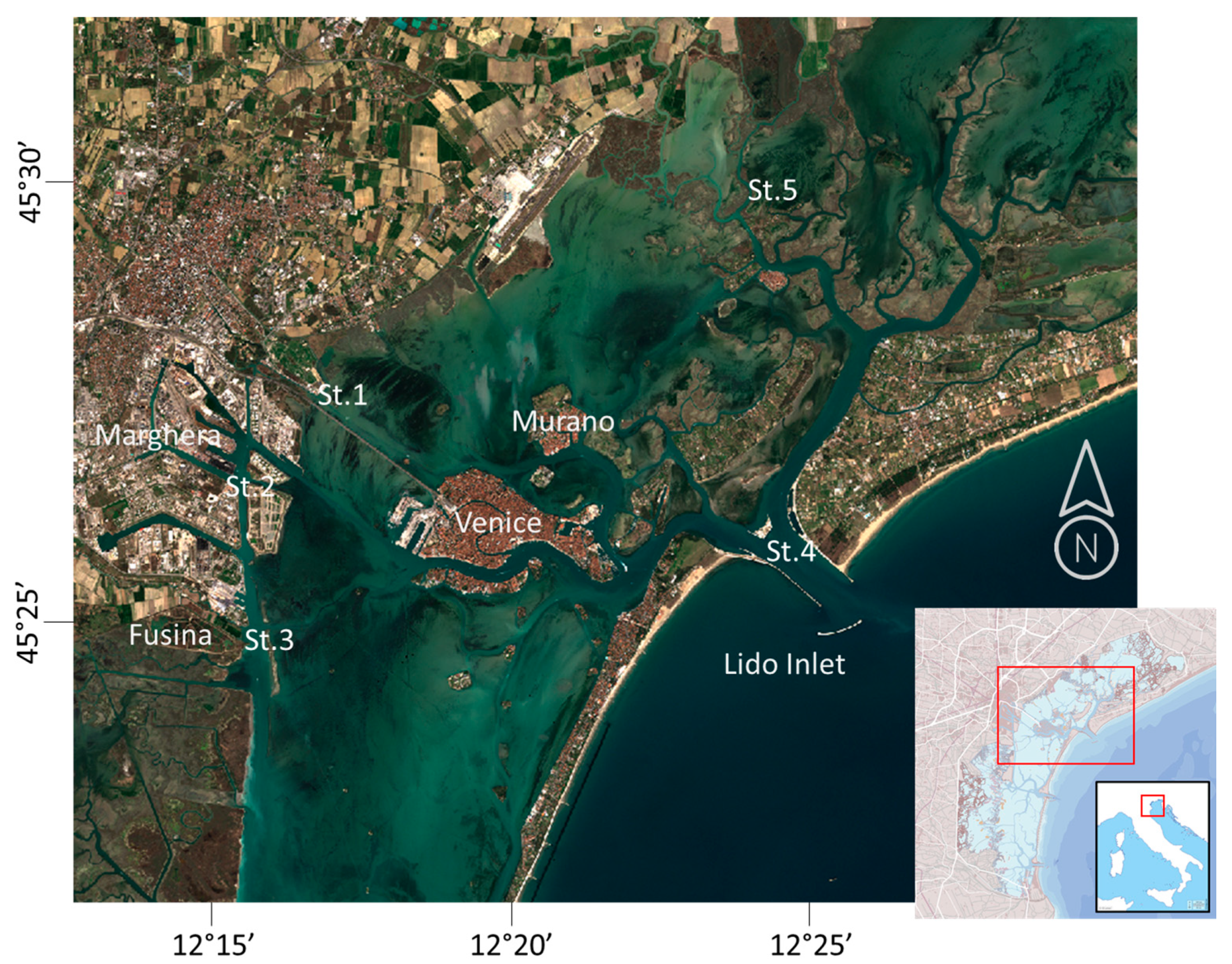
The VL (Figure 1) is a large (550 km²) Mediterranean coastal transitional environment located in Italy, in the Northeastern part of the Adriatic Sea. It has an average depth of 1 m, and it is morphologically characterized by the presence of canals (5–10 m deep) and of a multiplicity of aquatic (e.g., salt marshes, shoals, and mud flats) and terrestrial (e.g., islands, coastal strips) habitats. The VL is microtidal, poly- and euhaline, and, in terms of confinement, it has both choked and restricted waters [19]. Two long barrier islands separate the lagoon from the Adriatic Sea to the east, allowing for water exchange through three large inlets (Lido, Malamocco and Chioggia), each corresponding to a specific basin inside the lagoon (north, central and south). Water exchange in VL is governed by the Adriatic tides, whose average amplitude ranges between 20 cm at neap tides and 100 cm at spring tides. The average residence time of VL waters is around 10 days, varying from a few days close to the inlets to 30 days for the internal areas [20,21]. The yearly freshwater discharge in the VL, coming from twelve main tributaries, is about 35 m³ s⁻¹ on average, with seasonal peaks in spring and autumn. The VL is subjected to high levels of various anthropogenic pressures, due to the presence of urban areas, tourism, fishing, aquaculture, hydro-morphological interventions, industrial sites, and agricultural lands in the watershed. The five LV stations (Figure 1), where the long-term studies are carried on, are fairly well representative of the northern (St. 5) and central (Sts. 1, 2, 3 and 4) basins. The northern one is characterized by the presence of tributaries draining the waters from an intensively cultivated hinterland; the central one is subject to strong nutrient enrichment from the city of Venice and from the major islands, and it receives treated urban waste waters from the urban centre of Mestre and the discharge of wastewaters and cooling waters from the nearby industrial areas of Fusina and Marghera (Figure 1).

2.2. Sampling Strategy, Hydrochemical Parameters and Laboratory Methods

Monthly samplings were carried out from 1998 to 2017 at the near-surface layers of each station, at neap tide and prevalently in the morning, maintaining the duration of the whole operations as short as possible (around 4 h in total). For each parameter, we collected and analyzed one sample at each station. The parameters measured and the relative methods are reported in

Table 1. Investigated parameters, instruments and methods.

Parameters	Instruments and Methods
Transparency	Secchi Disck
Temperature	Bucket thermometer
Salinity	Guildline Autosal 8400B
	From 2012 multiparametric Idronaut mod. 801 and Sea-Bird SBE 19 plus.
Dissolved oxygen	Winkler’s method [22]
Inorganic dissolved nutrients	Systea-Alliance Continuous Flow Analyser. From 2007 Systea EasyChem Plus, [23]
Chlorophyll a	Perkin Elmer LS5B spectrofluorometer, [24]. From 2010 Turner Trilogy Laboratory Fluorometer.

. Analytical quality was assessed via participation in the Quality Assurance of Information for Marine Environmental Monitoring in Europe international laboratory proficiency-testing programme (QUASIMEME; http://www.quasimeme.org (accessed on 4 October 2021)).

Phytoplankton was fixed in neutralized formalin with hexamethylentetramine, recognized and counted with an invertoscope after samples had settled in 2–25-mL chambers, for 12–24 h. Cell counting was carried out at 400× magnification along transects, whose number varied depending on cell abundance, to count a minimum of 200 cells (but often more than 500) in each sample [25,26,27]. Over the study period, two different operators analyzed the phytoplankton samples using the same technique and with accurate intercalibration. Taxa composition was mainly defined in accordance with [28,29]. All the species were reviewed and conformed to any synonyms through the World Register of Marine Species WoRMS (https://www.marinespecies.org (accessed on 4 October 2021)) and the World’s Algae databases Algaebase, (http://www.algaebase.org/ (accessed on 4 October 2021)). The analysis was confined only to those forms that were detectable by light microscopy, i.e., up to 3 μm, thus not considering the picophytoplankton fraction. For a detailed analysis of interannual variations and trends, we focused only on the four major groups of phytoplankton: diatoms, nanoflagellates, dinoflagellates and coccolithophorids. For the dinoflagellates, no distinction has been made between autotrophic and heterotrophic species, which were therefore all included in the countings. The nanoflagellate group contained all the undetermined organisms, whose size was always less than 10 μm, mostly around 3–4 μm, mainly consisting of cryptophyceans, chrysophyceans, prymnesiophyceans (except coccolithophorids), chlorodendrophyceans and undetermined flagellates.

2.3. Phytoplankton Data Processing and Statistical Analyses

Statistical analyses were carried out on a matrix composed of 422 taxa and 1202 samples, after log-transformation of biological data [30] to account for non-normal data distributions [31].

Since the main focus of this study was the individuation of the overall features of the central and northern basins of the VL, we did not address any comparison among the single stations, which we pooled together to obtain an overall view of the area. Indeed, previous studies [13] evidenced that all stations shared the most abundant phytoplankton species and that taxonomic composition did not exhibit significant spatial differences.

We performed different types of analysis in order to: (i) identify the prevalent seasonal cycle and the most characteristic taxa or taxa assemblages in each season, (ii) assess the interannual variability and the long-term trends, and (iii) compare the water quality index MPI in the different years.

2.3.1. Annual and Seasonal Variations

The average phytoplankton seasonal cycle was assessed calculating the averages abundance of each month in the 20 years.

In order to identify the most characteristic species or species assemblages of each season, the Indicator Value (IndVal [32]), which combines the relative abundance of a species with its relative frequency of occurrence in a given seasonal period, was calculated on the seasonal average abundance. The IndVal is among the indicators most suitable to describe the average seasonal pattern of the plankton community, when a pluriannual set of data is available [13,33,34,35]. The higher the mean abundance and the relative frequency of occurrence of one species in a season, the higher the IndVal. These two terms are multiplied and then scaled to 100 to express the indicator value of a species with respect to the cluster in terms of percentages. The significance of the indicator values for each species was tested using a Monte Carlo permutation test (999 random permutations).

We adopted a conventional division of the seasons, which we defined as follows: January–March, winter; April–June, spring; July–September, summer; October–December, autumn. This division was used to calculate the IndVal and to individuate the taxa most typical in each season. In presenting the results, we evidenced whenever a taxa characterized different part of a season, with an early or late presence.

2.3.2. Interannual Variability and Pluriannual Trends

For providing an overview of phytoplankton interannual variability, we used a 12-month moving average. The pluriannual trends were analyzed by applying to the whole dataset a seasonal Kendall-tau nonparametric analysis following [36]. For the MPI, we performed the principal component analysis (PCA, R-mode) on the annual MPI values and on the yearly average values of each hydrochemical variable in order to identify their relationships and to display groups of observations in a 2-dimensional space. To assess the evolution of MPI, estimated every year, a simple Mann–Kendall test was used according to [37].

2.3.3. Multiparametric Phytoplankton Index

The MPI is an annual assessment of the water quality, which combines a diversity index (Menchinick’s Diversity, [38]) and a dominance index (Hulburt’s Dominance) with bloom frequency and chlorophyll-a concentration. The rationale behind the index and the detailed procedure for its application are reported in [8]; here, we give just the main information regarding the components of the index:

(i)

Hulburt’s index, the first metric, is a species dominance index, calculated as δ₂ = 100 (n₁ − n₂)/N_t, where n₁ is the abundance of the dominant species, n₂ is abundance of the second most abundant species, and N_t is the total abundance. In order to relate Hulburt’s index to water quality, the ‘‘100—δ₂’ value is used.

(ii)

Bloom frequency, the second metric, is the number of times in each year in which the abundance contribution of a single species exceeds the 50% of the total. The numerical value obtained is a percentage, and it is used as “100—Bloom Frequency”.

(iii)

Menhinick’s index, the third metric, is a diversity index calculated as D = S/√N, where S is the number of species and N is total abundance. To reduce the error caused by deletion of multiple indeterminate taxa, a correction factor was introduced, estimated as the ratio of the sum of the determinate taxa to the original total abundance (determinate + indeterminate taxa).

(iv)

Chlorophyll-a concentrations, the fourth metric, were obtained after log₁₀-transformation, removal of outliers (values outside the range |average ± 2.5 × std. dev.|) and calculation of antilogs.

Following the indications provided by the WFD, the range of the index was divided into five classes of ecological status, which were already adopted in [8], spanning from “bad” (eutrophic conditions with very low biodiversity, opportunistic phytoplankton species dominating the community, leading to very high chlorophyll-a concentrations) to high (communities characterized by high biodiversity and low chlorophyll-a): Bad: 0–0.2, Poor 0.21–0.4, Moderate 0.41–0.6, Good 0.61–0.8 and High 0.81–1.

3. Results

The range of the values of the physical and chemical variables in the 20 years (

Table 2. Averages (Avg) and standard deviations (SD), minimum (min) and maximum (max) values, and number of observations (n) for the main abiotic parameters for the whole study period.

		Avg	Min	Max	SD	n
Transparency	m	1.4	0.1	6.6	1.0	1169
Temperature	°C	18.2	0.6	33.9	7.5	1220
Salinity		28.62	8.63	37.05	4.79	1218
Relative Oxygen	%	105	38	204	18	1217
N-NH3	µM	8.74	0.01	69.23	9.30	1215
N-NO2	µM	1.49	0.02	11.93	1.11	1215
N-NO3	µM	32.49	0.01	211.14	28.51	1215
DIN	µM	42.71	0.52	242.97	33.74	1215
Si-SiO4	µM	33.20	0.83	294.15	30.99	1215
P-PO4	µM	0.79	0.01	17.19	0.96	1215
N/P		118	1	1889	161	1215
Chlorophyll-a	µg L−1	5.23	0.02	124.64	10.86	1214
Total Phytoplankton	Cells L−1	4,471,079	92,293	115,496,858	9,706,009	1202

), which have been thoroughly analyzed in [17], clearly testifies to the marked environmental heterogeneity of the features of the lagoon waters, as indicated by the variability of temperature (0.6 °C to 33.9 °C), salinity (8.63–37.05) and nutrients (dissolved inorganic nitrogen (DIN) 0.52–242.97 µM; Si-SiO₄ 0.83–294.15 µM; and P-PO₄ 0.01–17.19 µM).

The average total phytoplankton abundance was 4,471,079 cells L⁻¹ (SD 9,706,009 cells L⁻¹), with single values spanning several orders of magnitude, from a minimum of 92,293 cells L⁻¹ (February 2005) to a maximum of 115,496,858 cells L⁻¹ (August 2013).

We identified 422 distinct taxa belonging to 22 divisions: bacillariophyceae (diatoms; 262), dinophyceae (dinoflagellates; 62), chlorophyceae (42), prymnesiophyceae coccolithales (coccolithophorids; 15), chrysophyceae (5), euglenophyceae (5), cyanophyceae (5), dictyochophyceae (4), raphidophyceae (3), pyramimonadophyceae (3), cryptophyceae (2), thecophilosea (2), prymnesiophyceae (2), xantophyceae (2), chlorodendrophyceae (1) incertae sedis (1) trebouxiophyceae (1), kinetoplastea (1), choanoflagellatea (1), telonemia (1), katablepharidophyceae (1) and undetermined flagellates (1).

Phytoplankton abundance was overall mainly made up of diatoms (60% on the average), followed by nanoflagellates (37%), dinoflagellates (2%) and coccolithophorids (0.2%). The relevance of the other taxa was negligible (far below 0.1%).

3.1. Seasonal Pattern

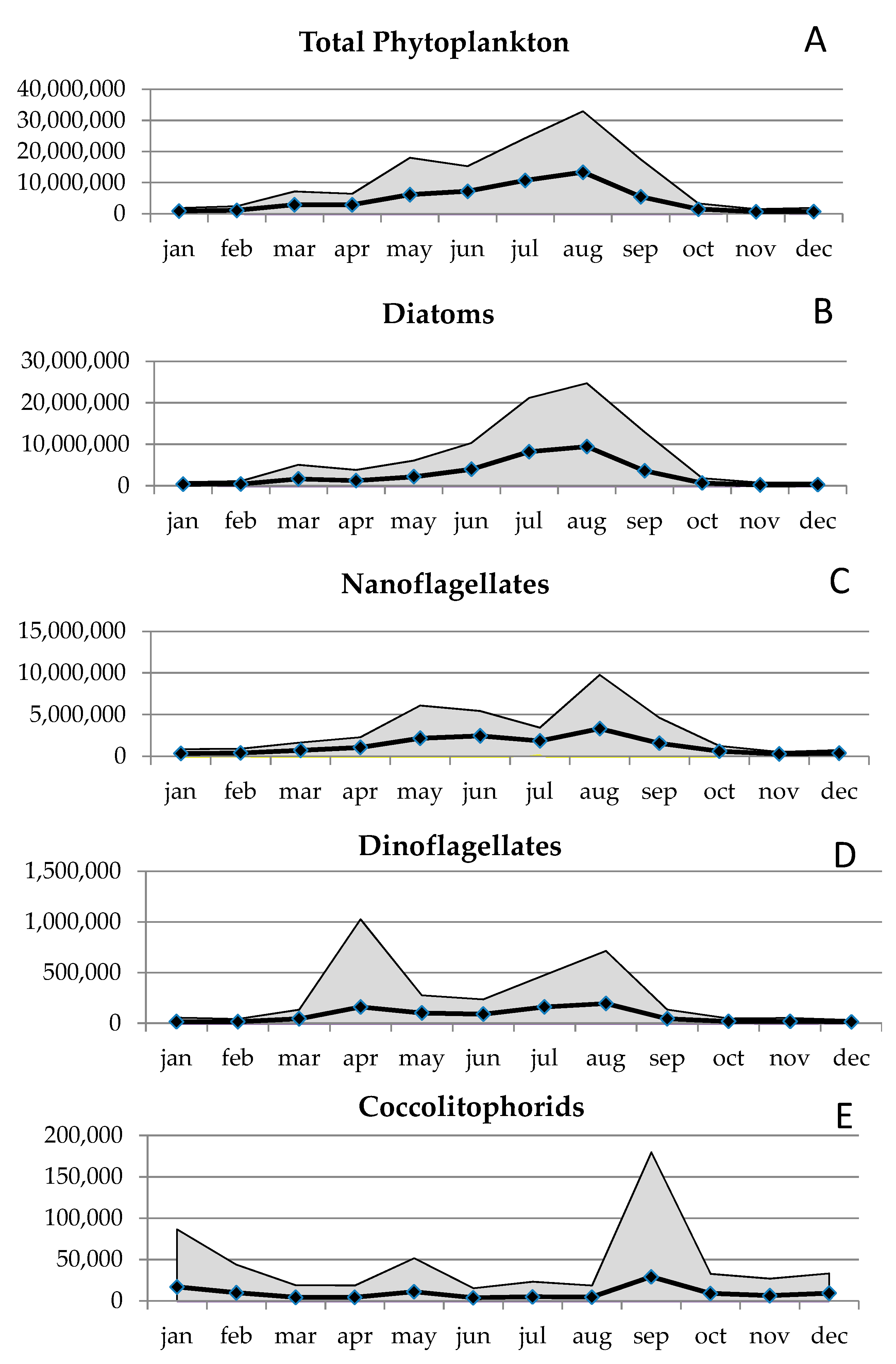
The average annual pattern of the total phytoplankton abundance (Figure 2a) showed the maximum values in summer (August) and the lowest in winter (January and December). Diatoms (Figure 2b) were numerically dominant throughout the time series, averaging 2,663,821 cells L⁻¹ (SD 7,337,630 cells L⁻¹), with marked seasonal variations. They were characterized by minor peaks in the late-winter period, by yearly maxima attained in summer, and then by a gradual decline in autumn, until reaching the lowest abundance typical of the winter conditions. As regards the species composition (

Table 3. List of main phytoplankton taxa characterized by the highest and significant IndVal for each season in the period 1998–2017. For each taxa, we also indicate the divisions to which they belong. IndVal values indicated with ** are significant at p < 0.01, and those with *** are significant at p < 0.001. Taxa are listed in order of decreasing importance in each season.

Division	Species	Winter	Spring	Summer	Autumn	p.
Diatoms	Skeletonema marinoi	25.422	8.072	6.889	1.23	***
Coccolithophorids	Emiliania huxleyi	15.535	1.816	2.563	7.873	***
Diatoms	Gyrosigma fasciola	7.010	0.549	0.201	1.381	**
Diatoms	Navicula tripunctata	6.899	0.187	0.127	0.339	***
Diatoms	Pseudo-nitzschia spp.	6.264	1.209	1.126	1.105	**
Diatoms	Melosira nummuloides	4.764	0.067	0.185	0.052	***
Diatoms	Melosira spp.	3.838	0.699	0.061	0.558	**
Diatoms	Amphora lineolata	3.318	0.046	0	0.359	***
Euglenophyceans	Eutreptia globulifera	2.744	0.011	0.048	0.006	**
Chrysophyceans	Dinobryon coalescens	1.780	0.042	0	0.003	**
Diatoms	Navicula spp.	17.216	27.320	15.792	12.772	***
Diatoms	Navicula cryptocephala	19.14	19.590	6.177	3.464	**
Dinoflagellates	Prorocentrum minimum	1.525	16.021	1.821	0.029	***
Diatoms	Cyclotella spp. (small)	0.872	13.394	11.494	0.919	**
Dinoflagellates	Prorocentrum gracile	0.005	5.293	0.346	0.803	***
Chlorophyceans	Ankistrodesmus spp.	0.066	4.590	2.237	0.679	**
Dinoflagellates	Prorocentrum triestinum	0.005	4.338	0.085	0.835	**
Diatoms	Halamphora hyalina	0.718	3.959	0	0.036	**
Diatoms	Licmophora gracilis	1.064	3.279	0.181	0.24	**
Diatoms	Cylindrotheca closterium	6.675	11.212	35.367	1.228	***
Diatoms	Thalassiosira spp. (small)	7.408	26.401	34.156	5.176	***
Diatoms	Nitzschia frustulum	0.144	2.616	24.245	1.448	***
Dinoflagellates	Und. naked dinoflagellates <20 µm	7.423	13.232	19.750	6.378	**
Diatoms	Thalassiosira pseudonana	0.096	5.991	19.339	0.503	***
Dinoflagellates	Gymnodinium spp.	2.109	11.775	16.092	1.9	***
Diatoms	Chaetoceros spp. (small)	3.79	12.593	15.323	0.354	***
Diatoms	Phaeodactylum tricornutum	0	0.921	14.151	0.021	***
Diatoms	Leptocylindrus minimus	0.044	0.537	11.127	0.054	***
Diatoms	Skeletonema tropicum	0	0.013	10.684	0.435	***
Chlorodendrophyceans	Tetraselmis spp.	0.005	7.896	9.811	0.177	***
Dinoflagellates	Blixaea quinquecornis	0	0.766	9.143	0.004	***
Pyramimonadophyceans	Pyramimonas spp.	0.818	6.497	9.142	0.413	**
Diatoms	Cyclotella caspia	0.108	3.686	8.122	0.17	***
Diatoms	Pseudo-nitzschia galaxiae	0.024	0.129	8.083	0.515	***
Diatoms	Cerataulina pelagica	0.245	3.732	7.352	1.034	**
Diatoms	Proboscia alata	0.005	0.26	6.998	0.314	***
Diatoms	Pseudo-nitzschia multistriata	0	0.785	5.710	0.115	***
Dinoflagellates	Protoperidinium bipes	0.103	0.183	5.168	0.002	***
Diatoms	Chaetoceros calcitrans	0.049	2.253	4.740	0.055	***
Diatoms	Chaetoceros compressus	0.444	0.106	4.364	0.01	***
Chlorophyceans	Scenedesmus quadricauda	0.126	2.013	4.142	0.212	**
Diatoms	Thalassiosira rotula	0.07	0.031	2.767	0.002	**
Dinoflagellates	Prorocentrum rhathymum	0	0	2.288	0	**
Trebouxiophyceans	Chodatella spp.	0	0.642	2.107	0.007	**
Coccolithophorids	Michaelsarsia adriatica	0	0	1.874	0.03	**
Diatoms	Chaetoceros diversus	0	0	1.307	0	**
Diatoms	Cocconeis spp.	5.98	8.847	2.881	14.869	**
Diatoms	Craticula cuspidata	0.009	0.021	0.019	2.753	**
Coccolithophorids	Calciosolenia murrayi	0	0	0	2.730	***
Diatoms	Placoneis elginensis	0.041	0.071	0.046	2.173	**
Diatoms	Sellaphora pupula	0.145	0.116	0	2.084	**
Diatoms	Coscinodiscus spp.	0	0	0	1.706	***

), resuspended species (Gyrosigma fasciola and Melosira spp.) characterized the beginning of the winter, whilst Skeletonema marinoi dominated the first phase of the growing season in late-winter, followed by resuspended diatoms (Navicula spp., Halamphora hyalina, Licmophora gracilis) and small (<10 µm) Cyclotella spp. in spring. The highest summer diatom peaks were mainly due to Cylindrotheca closterium, small (<10 µm) Thalassiosira spp. (undetermined species and T. pseudonana), small (<15 µm) pennate diatoms (Nitzschia frustulum and Phaeodactylum tricornutum) and small (<10 µm) forms of Chaetoceros spp., together with Pseudonitzschia spp. (P. galaxiae and P. multistriata), Leptocylindrus minimus and Skeletonema tropicum. Resuspended and benthic diatoms (Placoneis elginensis, Navicula spp. and Cocconeis spp.) typified the low autumn abundance. Some samples were also characterized by the presence, with low numbers, of rare species of allochthonous origin (Table 3): marine species such as Proboscia alata, Cerataulina pelagica, Leptocylindrus minimus and Pseudo-nitzschia spp. in summer and freshwater species in autumn (Craticula cuspidata and Sellaphora pupula) and winter (Navicula tripunctata and Amphora lineolata).

Nanoflagellates (Figure 2c) were second to diatoms as abundance throughout the time-series, averaging 1,333,818 cells L⁻¹ (SD 32,091,079 cells L⁻¹), and they were generally most abundant between April and September.

Dinoflagellates (Figure 2d) represented less than 2% of the total abundance, with an average of 72,496 cells L⁻¹ (SD 317,697 cells L⁻¹). Overall, they were generally most abundant in spring (April) and summer (August), although rarely exceeding 1 × 10⁶ cells L⁻¹, while during autumn and winter the abundances were the lowest, around 1–2 × 10⁴ cells L⁻¹. The peaks were due to Prorocentrum spp. (P. minimum, P. gracile and P. triestinum) in spring and naked species (small (<10 µm) undetermined species, Gymnodinium spp.), Blixaea quinquecornis, Protoperidinium bipes and Prorocentrum rhathymum in summer (Table 3).

Coccolithophorids, represented almost exclusively by Emiliania huxleyi (71% on average), were recorded in low numbers throughout the study (on average 9405 L⁻¹, SD 51,957 cells L⁻¹), with an average contribution to the total abundance of 0.2%. Emiliania huxleyi was responsible for both the absolute peak, recorded in September, and of the highest relative abundance, attained in winter (Figure 2e and Table 3). The summer and autumn samples were characterized also by the presence of Michaelsarsia adriatica and Calciosolenia murrayi, respectively (Table 3).

Other taxa reported in Table 3 are mostly rare and of allochthonous origin, their presence being a result of freshwater inputs: the euglenophyceans Eutreptia globulifera and the chrysophycean Dinobryon coalescens marked the winter period; Ankistrodesmus spp. (chlorophyceans) the spring; and Tetraselmis spp. (chlorodendrophyceans), Pyramimonas spp. (pyramimonadophyceans), Scenedesmus quadricauda (Chlorophyceans) and Chodatella spp. (trebouxiophyceans) the summer.

From early spring to late summer, we occasionally observed some species that may potentially trigger Harmful Algal Blooms (HAB), such as the dinoflagellates Alexandrium minutum, Dinophysis caudata, D. fortii, D. sacculus, Gonyaulax polygramma, G. spinifera and Prorocentrum rhathymum and the diatoms Halamphora coffeiformis, Pseudo-nitzschia delicatissima, P. pseudodelicatissima complex, P. fraudulenta, P. galaxiae and P. pungens. These species were recorded on average in 4% of the samples (varying between 0 and 15%) and with values rarely exceeding 1 × 10⁶ cells L⁻¹, contributing to a total abundance on average of less than 4%. Their highest values of abundance were found in summer, in accordance with the general pattern of phytoplankton growing season. Detrimental effects of these species were never recorded in the VL.

3.2. Interannual Variability and Long-Term Trends

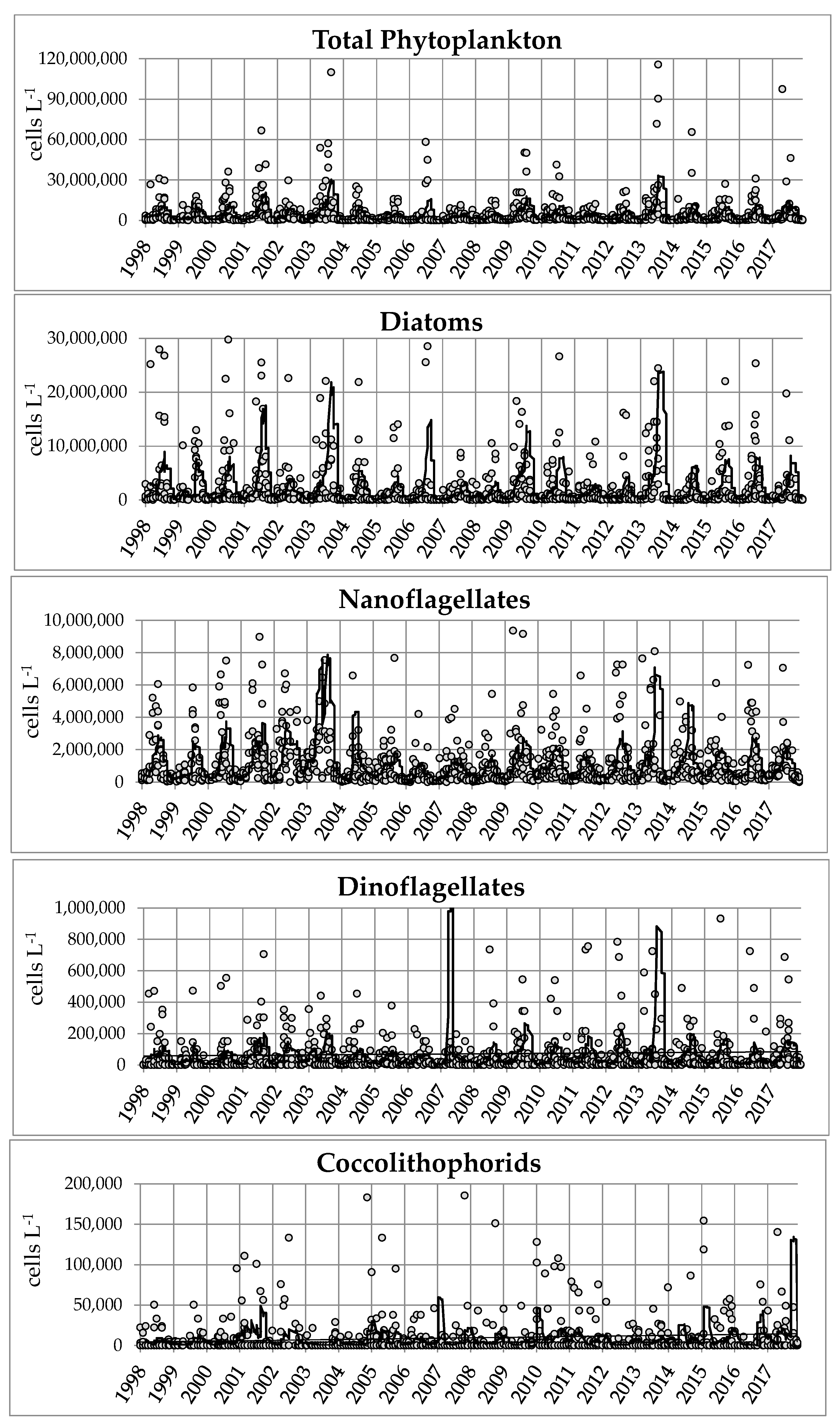
The yearly total phytoplankton abundance varied from 1,943,797 to 10,119,165 cell L^−1, and the changes were mainly determined by the yearly diatom variations (Figure 3). The diatoms peaks were always due to blooms, made by a few species: in 2001, Thalassiosira spp. and Cyclotella spp. in spring and Cylindrotheca closterium, Skeletonema tropicum and Nitzschia frustulum in summer. The year 2003 was characterized by summer blooms of Cyclotella spp., Thalassiosira spp. and Nitzschia frustulum; the year 2006 by an intense summer bloom of Thalassiosira spp. In 2009 and 2013, late winter blooms of Skeletonema marinoi occurred, which were followed in 2013 by summer blooms of a mixed community made by Chaetoceros spp., Thalassiosira spp. and Nitzschia frustulum. In the years with the lowest diatom abundance, this same pool of species was always responsible for blooms, even though they were far less intense.

The variation of the other phytoplankton groups was less marked (Figure 3): nanoflagellates were highest in 2003 and 2013, due to intense peaks (more than 20 × 10⁶ cells L⁻¹) from May to September, and lowest in 2006. Dinoflagellate abundance was highest in 2007, with undetermined naked forms (< 20 µm; up to 1 × 10⁶ cells L⁻¹) and in 2013 with Blixaea quinquecornis (up to 2 × 10⁶ cells L⁻¹), and it was lowest in 2006. Coccolithophorids peaked only in 2017 (1,237,703 cells L⁻¹ in late September).

For what concerns the long-term trend, the seasonal Kendall test evidenced negative slopes for the total phytoplankton abundance, for diatoms, nanoflagellates and dinoflagellates, and a positive one for coccolithophorids. All the trends, however, were not statistically significant. On the contrary, the MPI and each of its single four metrics showed statistically significant increasing trends: metric 1 (Mann–Kendall trend test: τ = 0.58; p < 0.05) and metric 3 (τ = 0.45; p < 0.05) highlighted an increase of biodiversity, metrics 2 (τ = 0.33; p < 0.05) a lower frequency of bloom and metric 4 a decreasing trend of phytoplankton chlorophyll-a (τ = 0.67; p < 0.05).

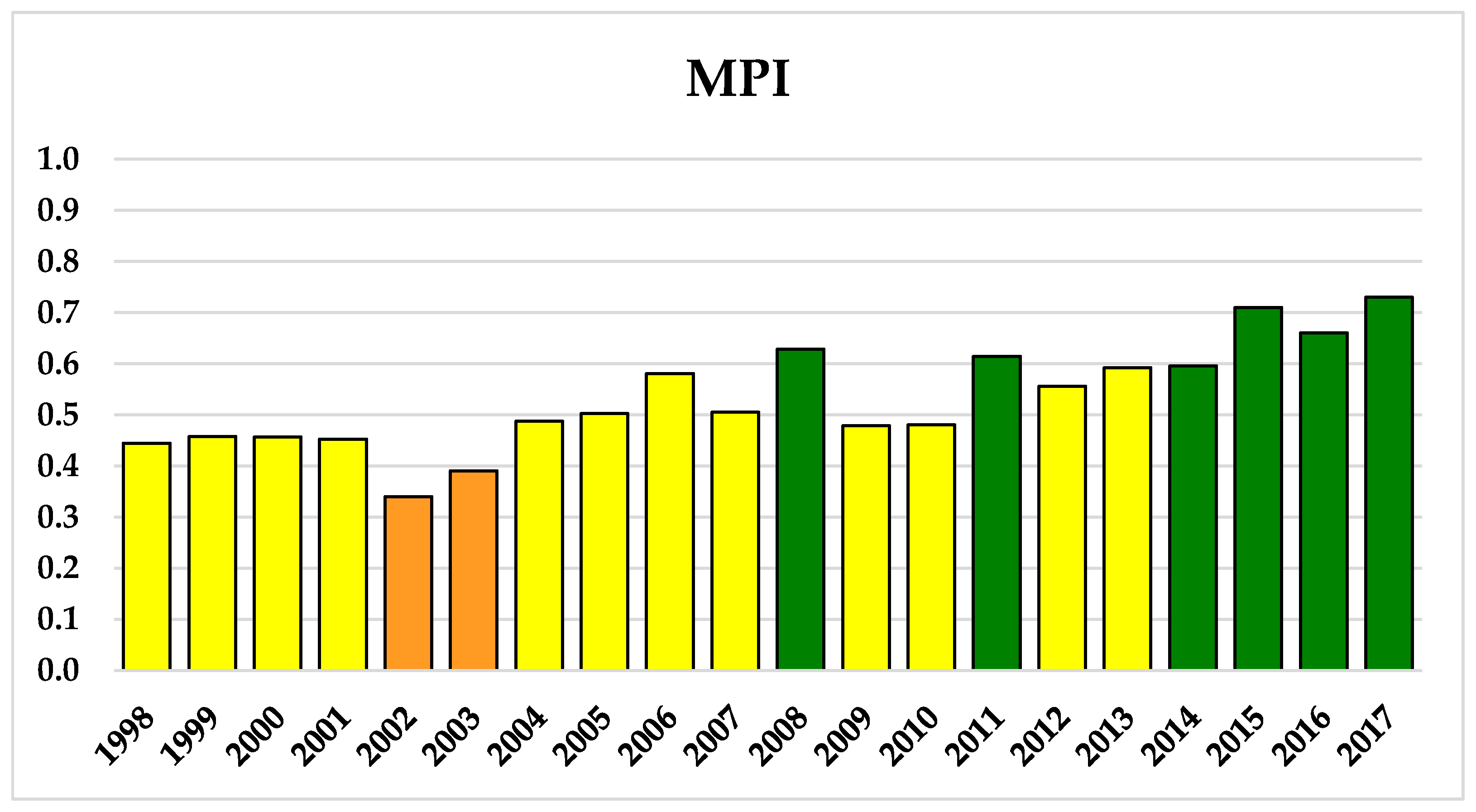
Indeed, the annual values of the MPI (Figure 4) showed a prevalence (12 years) of moderate conditions, with the frequency of good water quality levels increasing in the most recent years (2014–2017), while poor conditions were detected only twice (2002–2003) in the 20 years.

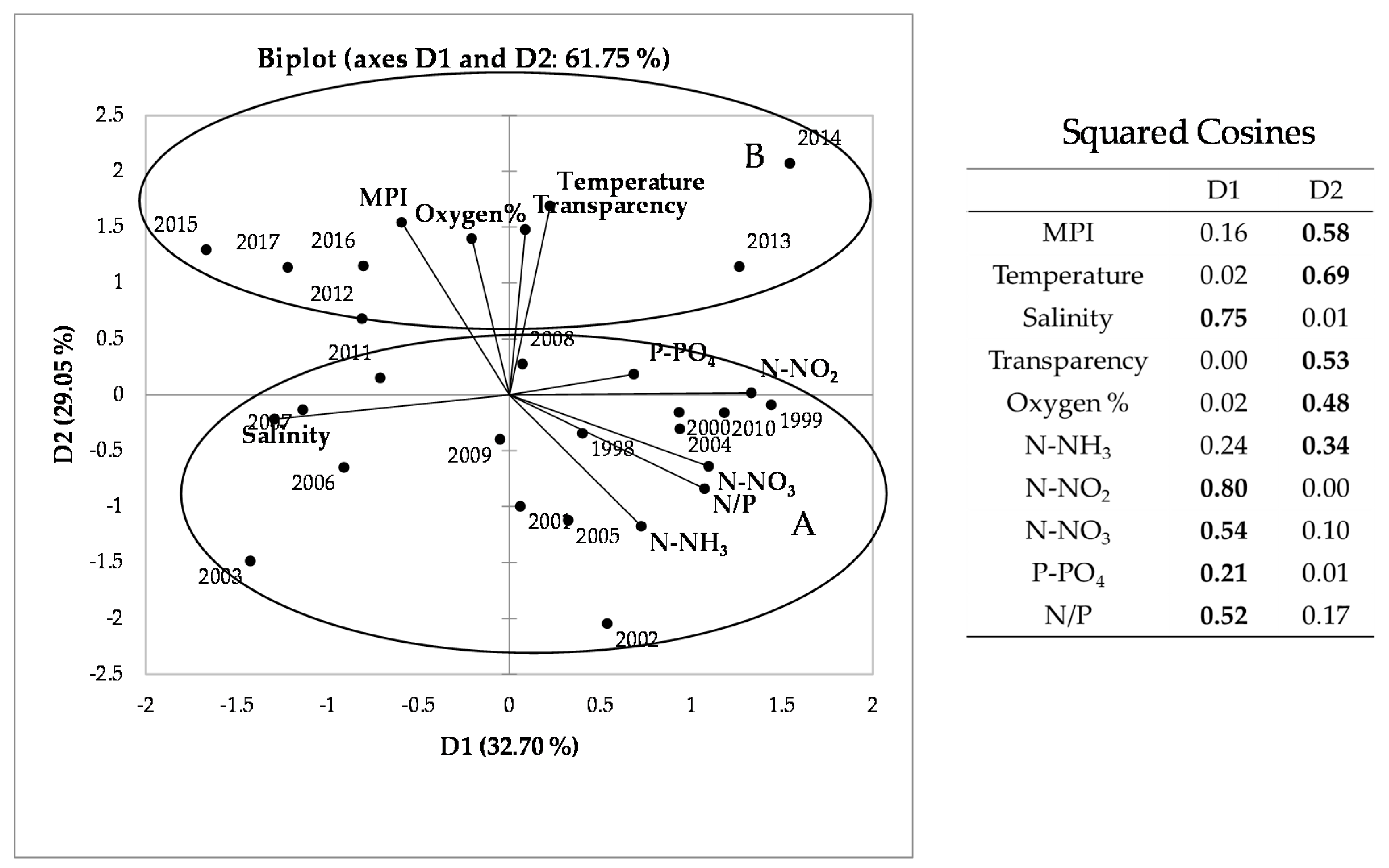
To investigate the relations of MPI with hydrochemical parameters, we performed a PCA (Figure 5). The bi-plot of the first two PCA components explained about 62% of the total variance. The squared cosine values identify the variables best linked to each of the two axes: the greater the squared cosine, the greater the link with the corresponding axis and, consequently, the influence of the variable along the axis. The first axis mainly explains the variability related, on one side, to salinity and, on the other, to nitrogen nutrients and N/P ratio. The second one explains the variability related to O₂ percentage, water transparency, water temperature and MPI, which are inversely correlated with N-NH₃ and N/P ratio. These variables allow evidencing in the PCA two clusters of consecutive years (

Table 4. Mann–Whitney test of the hydrochemical parameters [17], MPI, its four metrics and main blooming species, in the periods 1998–2011 and 2012–2017. SD, standard deviation; n, number of observations; p, probability level.

	1998–2011			2012–2017
	Mean	SD	n	Mean	SD	n	p
Transparency (m)	1.4	1.0	821	1.6	0.9	348	<0.01
Temperature (°C)	17.8	7.4	860	19.0	7.6	360	<0.02
Salinity	28.51	4.91	858	28.90	4.50	360	n.s.
Relative oxygen (%)	103	17	858	111	20	359	<0.01
N-NH4 (µM)	10.41	10.01	855	4.76	5.61	360	<0.01
N-NO2 (µM)	1.54	1.12	855	1.36	1.07	360	<0.01
N-NO3 (µM)	34.47	29.35	855	27.79	25.83	360	<0.01
P-PO4 (µM)	0.80	0.82	855	0.77	1.24	360	n.s.
N/P	127	160	855	98	160	360	<0.01
MPI-Metric 1 (Hulburt’s index)	0.52	0.09	14	0.65	0.07	6	<0.01
MPI-Metric 2 (blooms)	0.63	0.09	14	0.75	0.11	6	<0.01
MPI-metric 3 (Menhinick’s index)	0.38	0.12	14	0.44	0.09	6	n.s
MPI-metric 4 (Chlorophyll-a)	0.42	0.13	14	0.71	0.13	6	<0.01
MPI	0.49	0.08	14	0.64	0.07	6	<0.01
Skeletonema spp. (cells L−1)	442,035	2,034,888	843	259,231	1,133,632	359	<0.01
Chaetoceros spp. (small) (cells L−1)	101,620	536,888	843	246,824	1,264,153	359	<0.01
Nitzschia spp. (small) (cells L−1)	434,811	3,277,238	843	291,993	2,083,798	359	<0.01
Thalassiosira spp. (small) (cells L−1)	875,037	4,129,117	843	923,172	4,585,224	359	<0.01
Cylindrotheca closterium (cells L−1)	168,023	1,233,321	843	132,962	1,669,711	359	<0.01
Cyclotella spp. (small) (cells L−1)	205,569	1,533,757	843	48,150	279,220	359	n.s.

and Figure 5): cluster A and cluster B that group, respectively, the first 14 years (1998–2011) and the most recent ones (2012–2017). The division of these two groups occurs at the value 0.5 of the second component. The ordering of the years in relation to the first two main components appears to be fairly consistent with the MPI values (Figure 4) that appear to be the highest in well-oxygenated, transparent and less nutrient-rich waters. Indeed, the comparison of the two periods (Figure 5 and Table 4) indicated statistically significant differences for transparency, temperature and relative oxygen, which were highest in the second period. As regards nutrients, ammonium, nitrites and nitrates decreased significantly in recent years, resulting as well in a lower N/P ratio [17]. These changes in environmental variables were accompanied by an increase of the water quality assessed with MPI, which was significantly higher in the most recent years (2012–2017). For what concern the bloom species, three of them decreased (Skeletonema spp., small Nitzschia spp., Cylindrotheca closterium), while two (small Chaetoceros spp. and Thalassiosira spp.) increased.

4. Discussion

This paper could be considered as a “third episode of a series” addressing the changes of the water quality in the VL within the same 20-year period (1998–2017), from different points of view. Actually, two previous papers analyzed the VL water quality considering, respectively, (i) the abiotic parameters and the chlorophyll-a [17], and (ii) the relations between phytoplankton and macrophytes [14]. They both evidenced an overall improvement of the lagoon water quality, which seemed to enter a new phase in the most recent years. This phase is characterized, in particular, by a reduction in the trophic state [17], mainly related to lower inputs of inorganic dissolved nitrogen nutrients from the basin—which followed the Council Directive 91/676/EC introducing good agricultural practices concerning the prohibition of spreading nitrogen rich farm wastes—and by an increase in water transparency and dissolved oxygen, also related to the augmented biomass of both macroalgae and seagrasses, which started recolonizing the lagoon, boosted by the clam fishing regulation [14].

In this paper, following and grounded in the information coming from the former two, we focused only on the phytoplankton communities, examining their composition, seasonal patterns and trends, and addressing their use for the assessment of the changes in the water quality through time. This last issue, in particular, was tackled through the application of the multiparametric index MPI [8], based on phytoplankton biodiversity, chlorophyll-a and bloom frequency, which was specifically developed in the VL and, then, became an effective tool adopted by the Italian Ministry, local authorities, Greece, and Croatia to adhere to WFD requirements [11].

It is well known that long-term research is a unique tool for obtaining a consistent picture of the annual cycle of phytoplankton communities and for assessing trends and shifts [39,40,41,42,43]. Long-term series are crucial for revealing and interpreting the pattern of changes in phytoplankton biomass and composition, in particular in transitional environments, where an intrinsically high spatial and temporal heterogeneity characterizes phytoplankton, making its characterization and the consequent development of adequate indicators quite difficult [6,44,45,46]. In this respect, long-term series also appear essential to provide a robust base for assessing water quality changes as required by the WFD, which explicitly mentions the composition, abundance, frequency and intensity of algal blooms and biomass as phytoplankton quality elements in coastal and transitional waters [3].

Our study confirmed some features of the LV phytoplankton communities, which were already previously evidenced by a study based on a 10-year period [13]. First of all, the prevalent unimodal annual pattern of phytoplankton abundance, with a typical summer peak, was observed also in the present study. This pattern characterizes temperate enclosed coastal ecosystems, with shallow depths and permanently high nutrient concentrations [16]: the observed decrease in nutrient availability in the VL did not seem to affect the phytoplankton unimodal cycle, so that the seasonal climate cycle still remains the most recognizable driver of phytoplankton. This seasonal pattern is mainly driven by the diatoms, which are so far the most prevalent phytoplankton group in the lagoon, as typical of permanently fertile and turbulent environments [2,47]). Actually, diatoms are—from one perspective—the main responsible for the annual blooms in the VL, which occur each year mainly in late winter/spring and summer; from another, they are inclusive of taxa that represent the different systems (rivers, sea and sediments) connected with the lagoon waters. Blooms, which are essential features of many transitional ecosystems, are prevalently associated with diatoms due to their capacity to grow rapidly in turbulent high-nutrient environments [48]. Diatoms also dominate the phytoplankton in many other Mediterranean lagoons [49,50,51,52,53], and some of the genera responsible for blooms in the VL (i.e., Skeletonema, Thalassiosira and Chaetoceros) are key species known to produce blooms in transitional waters globally [48].

The second most abundant phytoplankton group in the VL is a taxonomically heterogeneous one, composed of undetermined flagellates with a size lower than 10 μm, which constitute on average almost the 40% of the total abundance in the lagoon. Undetermined nanoflagellates are also a typical and relevant component of other transitional environments [54,55,56,57,58]. In the VL, they contribute to the spring and summer peaks, and they represent a quite stable and important component throughout the years. Nanoflagellates are difficult or impossible to identify with light microscopy and in routine phytoplankton long-term monitoring they will very likely always be left undetermined, so that an important part of the phytoplankton biodiversity will remain hidden. Actually, recent studies on the VL protists through metabarcoding [59,60] revealed that nanoflagellates are represented by several distinct species, some of which (e.g., Picochlorum, Micromonas) were reported for the first in the lagoon in that study.

The average composition of the phytoplankton seasonal cycle in the VL (Table 3) is still quite comparable with that described for the previous ten-year period 1998–2007 [13]: diatom species imported from the benthic community (resuspended species, in particular Navicula spp., Amphora spp. and Cocconeis spp.) and coccolithophorids from the coastal sea (Calciosolenia murrayi, Emiliana huxleyi) typify the periods of lowest abundance (autumn and early winter). Planktonic diatoms (Skeletonema marinoi), together with Cyclotella spp. and some resuspended species (Amphora spp., Navicula spp., Lichmophora spp.), prevail in late winter and spring, together with a few dinoflagellates species (Prorocentrum spp.). In summer the species composition become characterized by a mixed assemblage of diatoms (Chaetoceros spp., Thalassiosira spp., Cylindrotheca Closterium and Nitzschia frustulum), which remain dominant, together with dinoflagellates (Gymnodinium spp., Protoperidinium bipes).

The trends of the total abundance and of each of the four main taxa appeared to decrease in the 20 years, although not in a statistically significant way, thus providing a weak signal that they are related to water quality improvement. A quite univocal sign came, instead, from the temporal variations of the MPI, which showed a statistically significant increasing trend, as a whole and in each single component. The value of the index shifted from the prevalent “moderate” quality class, which characterized the former years (until 2010), to the “good” class, which appeared quite stable since 2011. Blooms, chlorophyll-a, and biodiversity, when pooled together, seem to represent a most powerful tool to address the changes in water quality in the lagoon. The possibility to successfully apply the MPI has been tested, until now, only to compare spatially different areas of the same ecosystem or different lagoons [8,9], in particular due to its sensitivity to the water trophic conditions. In this work, we also provide evidence of the possibility to use it to compare the water quality changes over time, a necessary requisite to evaluate the effectiveness of restoration measures, in particular in relation to the WFD. It is worth noticing that the index appears to work effectively, even in the presence of many undetermined taxa, as is the case of the nanoflagellate component in the VL.

The MPI actually proved to be well correlated with the abiotic parameters in the VL, showing the highest value in well-oxygenated and less nutrient-rich waters. This correlation also allowed one, through the use of PCA, to separate two clusters of years (1998–2011; 2012–2017), the most recent ones characterized by improved water quality conditions. A statistically significant decrease in the frequency of the blooms was recorded comparing the two groups of years, even though there is not a univocal tendency among the taxa that typically cause them: actually, some, such as Cylindrotheca, Nitzschia and Skeletonema, decreased, while others (i.e., Thalassiosira and Chaetoceros) increased and, overall, the very same taxa were always mainly responsible for the blooms, whatever their intensity.

In conclusion, we wish to highlight that a general water quality improvement has taken place in the VL in the 20-year period 1998–2017, in particular for what concerns the trophic conditions and the recovery of the macrophytes. The single signals of changes in the phytoplankton communities were somewhat weak: as already evidenced in the past, the prevalent unimodal pattern of seasonal variation, the diatoms as dominant group and the wide interannual variability remained the typical unchanged features of the communities, which did not show a statistically significant decreasing trend of abundance over the years. The MPI, which pools together different features of the phytoplankton, appears instead to robustly confirm its reliability to address the changes in the water quality, not only spatially—as previously known—but also for following the yearly time trends. A multi-metric index that considers as many fundamental attributes of phytoplankton as possible (e.g., biomass, community structure and frequency of blooms) is indeed considered more sensitive and robust than the use of single metrics in assessing the status of transitional water ecosystems [7,46,58] and its spatial and temporal variations. This is particularly relevant considering that the trajectories of coastal ecosystems during oligotrophication may be more complex than expected as different controlling factors may change at the same time [61,62].

References

- Winder, M.; Cloern, J.E. The annual cycles of phytoplankton biomass. Phil. Trans. R. Soc. B 2010, 365, 3215–3226. [Google Scholar] [CrossRef]
- Cloern, J.E.; Jassby, A.D. Complex seasonal patterns of primary producers at the land-sea interface. Ecol. Lett. 2008, 11, 1–10. [Google Scholar] [CrossRef] [PubMed]
- European Commission. Directive 2000/60/EC of the European Parliament and of the Council of 23 October 2000 Establishing a Framework for Community Action in the Field of Water Policy (Water Framework Directive). Off. J. Eur. Union 2000, 43, 1–73. Available online: https://eur-lex.europa.eu/eli/dir/2000/60/oj (accessed on 4 October 2021).
- Facca, C.; Sfriso, A. Phytoplankton in a transitional ecosystem of the Northern Adriatic Sea and its putative role as an indicator for water quality assessment. Mar. Ecol. 2009, 30, 462–479. [Google Scholar] [CrossRef]
- Pereira Coutinho, M.T.; Brito, A.C.; Pereira, P.; Gonçalves, A.S.; Moita, M.T. A phytoplankton tool for water quality assessment in semi-enclosed coastal lagoons: Open vs. closed regimes. Estuar. Coast. Shelf. Sci. 2012, 110, 134–146. [Google Scholar] [CrossRef]
- Lugoli, F.; Garmendia, M.; Lehtinen, S.; Kauppila, P.; Moncheva, S.; Revilla, M.; Roselli, L.; Slabakova, N.; Valencia, V.; Dromph, K.M.; et al. Application of a new multi-metric phytoplankton index to the assessment of ecological status in marine and transitional waters. Ecol. Indic. 2012, 23, 338–355. [Google Scholar] [CrossRef]
- Garmendia, M.; Borja, A.; Franco, J.; Revilla, M. Phytoplankton composition indicators for the assessment of eutrophication in marine waters: Present state and challenges within the European directives. Mar. Pollut. Bull. 2013, 66, 7–16. [Google Scholar] [CrossRef] [PubMed]
- Facca, C.; Bernardi Aubry, F.; Socal, G.; Ponis, E.; Acri, F.; Bianchi, F.; Giovanardi, F.; Sfriso, A. Description of a Multimetric Phytoplankton Index (MPI) for the assessment of transitional waters. Mar. Pollut. Bull. 2014, 79, 145–154. [Google Scholar] [CrossRef] [PubMed]
- Bazzoni, A.M.; Pulina, S.; Padedda, B.M.; Satta, C.T.; Lugliè, A.; Sechi, N.; Facca, C. Water quality evaluation in Mediterranean lagoons using the Multimetric Phytoplankton Index (MPI): Study cases from Sardinia. Transit. Waters Bull. 2013, 7, 64–76. [Google Scholar]
- European Commission. Commission Decision (EU) 2018/229 of 12 February 2018 Establishing, Pursuant to Directive 2000/60/EC of the European Parliament and of the Council, the Values of the Member State Monitoring System Classifications as a Result of the Intercalibration Exercise and Repealing Commission Decision 2013/480/EU (Notified under Document C(2018) 696). Text with EEA Relevance. Available online: http://data.europa.eu/eli/dec/2018/229/oj (accessed on 4 October 2021).
- Francé, J.; Varkitzi, I.; Stanca, E.; Cozzoli, F.; Skejić, S.; Ungaro, N.; Vascotto, I.; Mozetič, P.; Ninčević Gladan, Z.; Assimakopoulou, G.; et al. Large-scale testing of phytoplankton diversity indices for environmental assessment in Mediterranean sub-regions (Adriatic, Ionian and Aegean Seas). Ecol. Indic. 2021, 126, 107630. [Google Scholar] [CrossRef]
- Bianchi, F.; Acri, F.; Aubry, F.B.; Berton, A.; Boldrin, A.; Camatti, E.; Cassin, D.; Comaschi, A. Can plankton communities be considered as bio-indicators of water quality in the lagoon of Venice? Mar. Pollut. Bull. 2003, 46, 964–971. [Google Scholar] [CrossRef]
- Bernardi Aubry, F.; Acri, F.; Bianchi, F.; Pugnetti, A. Looking for patterns in the phytoplankton community of the Mediterranean microtidal Venice Lagoon: Evidence from ten years of observations. Sci. Mar. 2013, 77, 47–60. [Google Scholar] [CrossRef] [Green Version]
- Bernardi Aubry, F.; Acri, F.; Scarpa, G.M.; Braga, F. Phytoplankton–Macrophyte Interaction in the Lagoon of Venice (Northern Adriatic Sea, Italy). Water 2020, 12, 2810. [Google Scholar] [CrossRef]
- Bernardi Aubry, F.; Pugnetti, A.; Roselli, L.; Stanca, E.; Acri, F.; Finotto, S.; Basset, A. Phytoplankton morphological traits in a nutrient-enriched, turbulent Mediterranean microtidal lagoon. J. Plankton Res. 2017, 39, 564–576. [Google Scholar] [CrossRef]
- Cebrian, C.; Valiela, I. Seasonal patterns in phytoplankton biomass in coastal ecosystems. J. Plankton Res. 1999, 21, 429–444. [Google Scholar] [CrossRef] [Green Version]
- Acri, F.; Braga, F.; Bernardi Aubry, F. Long-term dynamics in nutrients, chlorophyll a and water quality parameters in the Lagoon of Venice. Sci. Mar. 2020, 84, 215–225. [Google Scholar] [CrossRef]
- Sfriso, A.; Buosi, A.; Mistri, M.; Munari, C.; Franzoi, P.; Sfriso, A.A. Long-term changes of the trophic status in transitional ecosystems of the northern Adriatic Sea, key parameters and future expectations: The lagoon of Venice as a study case. Nat. Conserv. 2019, 34, 193–215. [Google Scholar] [CrossRef]
- Kjerfve, B.; Magill, K.E. Geographic and hydrodynamic characteristics of shallow coastal lagoons. Mar. Geol. 1989, 88, 187–199. [Google Scholar] [CrossRef]
- Umgiesser, G.; Ferrarin, C.; Cucco, A.; De Pascalis, F.; Bellafiore, D.; Ghezzo, M.; Bajo, M. Comparative hydrodynamics of 10 Mediterranean lagoons by means of numerical modeling. J. Geophys. Res. Oceans 2014, 119, 2212–2226. [Google Scholar] [CrossRef]
- Ghezzo, M.; De Pascalis, F.; Umgiesser, G.; Zemlys, P.; Sigovini, M.; Marcos, C.; Pérez-Ruzafa, A. Connectivity in three European coastal lagoons. Estuar. Coasts 2015, 38, 1764–1781. [Google Scholar] [CrossRef]
- Strickland, J.D.H.; Parsons, T.R. A Practical Handbook of Seawater Analysis, 2nd ed.; Bulletin 167; Alger Press Ltd.: Ottawa, ON, Canada, 1972; pp. 1–310. [Google Scholar]
- Grasshoff, K.; Ehrhardt, M.; Kremling, K. (Eds.) Methods of Seawater Analysis, 2nd ed.; rev. and extended ed.; Wiley, Verlag Chemie: Weinheim, Germany, 1983; p. 419. [Google Scholar]
- Holm-Hansen, O.; Lorenzen, C.J.; Holmes, R.W.; Strickland, J.D.H. Fluorometric determination of chlorophyll. ICES J. Mar. Sci. 1965, 30, 3–15. [Google Scholar] [CrossRef]
- Uthermöhl, H. Zur Vervollkomnung der quantitativen, Phytoplankton-Methodik. Mitt. Int. Ver. Limnol. 1958, 9, 1–38. [Google Scholar]
- Throndsen, J. Preservation and storage. Phytoplankton Manual. In Monographs on Oceanographic Methodology; Sournia, A., Ed.; UNESCO: Paris, France, 1978; Volume 6, pp. 69–74. [Google Scholar]
- Zingone, A.; Totti, C.; Sarno, D.; Cabrini, M.; Caroppo, C.; Giacobbe, M.G.; Luglié, A.; Nuccio, C.; Socal, G. Fitoplancton: Metodiche di analisi quali-quantitativa. In Metodologie di Studio del Plancton Marino. Manuali e Linee Guida 56/2010; Socal, G., Buttino, I., Cabrini, M., Mangoni, O., Penna, A., Totti, C., Eds.; ISPRA SIBM: Roma, Italy, 2010; pp. 213–237. [Google Scholar]
- Tomas, C.R. Identifying Marine Phytoplankton; Academic Press, Arcourt Brace & Company: Cambridge, MA, USA, 1997. [Google Scholar]
- Berard-Therriault, L.; Poulin, M.; Bossé, L. Guide D’Identification du Phytoplancton Marin de L’Estuaire et du Golfe du Saint-Laurent; NRC Research Press: Ottawa, ON, Canada, 1999; 387p. [Google Scholar]
- Cassie, R.M. Frequency distribution model in the ecology of plankton and other organisms. J. Anim. Ecol. 1962, 31, 65–92. [Google Scholar] [CrossRef]
- Sokal, R.; Rohlf, J. Biometry: The Principles and Practice of Statistics in Biological Research, 2nd ed.; W.H. Freeman: San Francisco, CA, USA, 1981; p. 859. [Google Scholar]
- Dufrêne, M.; Legendre, P. Species assemblages and indicator species: The need for a flexible asymmetrical approach. Ecol. Monogr. 1997, 67, 345–366. [Google Scholar] [CrossRef]
- Bernardi Aubry, F.; Cossarini, G.; Acri, F.; Bastianini, M.; Bianchi, F.; Camatti, E.; De Lazzari, A.; Pugnetti, A.; Solidoro, C.; Socal, G. Plankton communities in the northern Adriatic Sea: Patterns and changes over the last 30 years. Estuar. Coast. Shelf. Sci. 2012, 115, 125–137. [Google Scholar] [CrossRef]
- Cerino, F.; Fornasaro, D.; Kralj, M.; Giani, M.; Cabrini, M. Phytoplankton temporal dynamics in the coastal waters of the north-eastern Adriatic Sea (Mediterranean Sea) from 2010 to 2017. Nat. Conserv. 2019, 34, 343–372. [Google Scholar] [CrossRef]
- Totti, C.; Romagnoli, T.; Accoroni, S.; Coluccelli, A.; Pellegrini, M.; Campanelli, A.; Grilli, F.; Marini, M. Phytoplankton communities in the northwestern Adriatic Sea: Interdecadal variability over a 30-years period (1988–2016) and relationships with meteoclimatic drivers. J. Mar. Syst. 2019, 193, 137–153. [Google Scholar] [CrossRef]
- Hirsch, R.M.; Alexander, R.B.; Smith, R.A. Selection of methods for the detection and estimation of trends in water quality. Water Resour. Res. 1991, 27, 803–813. [Google Scholar] [CrossRef]
- Gilbert, R.O. Statistical Methods for Environmental Pollution Monitoring; Van Nostrand Reinhold: New York, NY, USA, 1987; p. 320. [Google Scholar]
- Spatharis, S.; Tsirtsis, G. Ecological quality scales based on phytoplankton for the implementation of Water Framework Directive in the Eastern Mediterranean. Ecol. Indic. 2010, 10, 840–847. [Google Scholar] [CrossRef]
- Long-Term Phytoplankton Time Series. Time series data relevant to eutrophication and ecological quality indicators (WKEUT). In Journal of Sea Research. Special Issue; Borkman, D., Baretta-Bekker, H., Henriksen, P., Eds.; Elsevier: Amsterdam, The Netherlands, 2009; Volume 61, pp. 1–124. [Google Scholar]
- Briand, F. (Ed.) Phytoplankton responses to Mediterranean environmental changes. In CIESM Workshop Monographs; CIESM Publisher: Monaco, 2010; Volume 40, pp. 1–120. [Google Scholar]
- Edwards, M.; Beaugrand, G.; Hays, G.C.; Koslow, J.A.; Richards, A.J. Multi-decadal oceanic ecological datasets and their application in marine policy and management. Trends Ecol. Evol. 2010, 25, 602–610. [Google Scholar] [CrossRef]
- Klais, R.; Cloern, J.E.; Harrison, P.J. Global Patterns of Phytoplankton Dynamics in Coastal Ecosystems. Estuar. Coast. Shelf Sci. 2015, 162, 1–160. [Google Scholar]
- Morabito, G.; Mazzocchi, M.; Salmaso, N.; Zingone, A.; Bergami, C.; Flaim, G.; Accoroni, S.; Basset, A.; Bastianini, M.; Belmonte, G.; et al. Plankton dynamics across the freshwater, transitional and marine research sites of the LTER-Italy Network. Patterns, fluctuations, drivers. Sci. Total Environ. 2018, 627, 373–387. [Google Scholar] [CrossRef] [PubMed]
- Devlin, M.; Best, M.; Coates, D.; Bresnan, E.; O’Boyle, S.; Park, R.; Silke, J.; Cusack, C.; Skeats, J. Establishing boundary classes for the classification of UK marine waters using phytoplankton communities. Mar. Pollut. Bull. 2007, 55, 91–103. [Google Scholar] [CrossRef] [PubMed]
- Henriksen, P. Reference conditions for phytoplankton at Danish Water Framework Directive intercalibration sites. Hydrobiologia 2009, 629, 255–262. [Google Scholar] [CrossRef]
- Leruste, A.; Villéger, S.; Malet, N.; De Wit, R.; Bec, B. Complementarity of the multidimensional functional and the taxonomic approaches to study phytoplankton communities in three Mediterranean coastal lagoons of different trophic status. Hydrobiologia 2018, 815, 207–227. [Google Scholar] [CrossRef] [Green Version]
- Margalef, R. Life-forms of phytoplankton as survival alternatives in an unstable environment. Oceanol. Acta 1978, 1, 493–509. [Google Scholar]
- Carstensen, J.; Klais, R.; Cloern, J.E. Phytoplankton blooms in estuarine and coastal waters: Seasonal patterns and key species. Estuar. Coast. Shelf Sci. 2015, 162, 98–109. [Google Scholar] [CrossRef] [Green Version]
- Sarno, D.; Zingone, A.; Saggiomo, V.; Carrada, G.C. Phytoplankton biomass and species composition in a Mediterranean coastal lagoon. Hydrobiologia 1993, 271, 27–40. [Google Scholar] [CrossRef]
- Caroppo, C. The contribution of picophytoplankton to community structure in a Mediterranean brackish environment. J. Plankton Res. 2000, 22, 381–397. [Google Scholar] [CrossRef]
- Nuccio, C.; Melillo, C.; Massi, L.; Innamorati, M. Phytoplankton abundance, community structure and diversity in the eutrophicated Orbetello lagoon (Tuscany) from 1995 to 2001. Oceanol. Acta 2003, 26, 15–25. [Google Scholar] [CrossRef] [Green Version]
- Fanuko, N.; Valcic, M. Phytoplankton composition and biomass of the Northern Adriatic lagoon Stella Maris, Croatia. Acta Bot. Croat. 2009, 68, 29–44. [Google Scholar]
- Derolez, V.; Soudant, D.; Malet, N.; Chiantella, C.; Richard, M.; Abadie, E.; Aliaume, C.; Bec, B. Two decades of oligotrophication: Evidence for a phytoplankton community shift in the coastal lagoon of Thau (Mediterranean Sea, France). Estuar. Coast. Shelf Sci. 2020, 241, 106810. [Google Scholar] [CrossRef]
- Glibert, P.M.; Boyer, J.N.; Heil, C.; Madden, C.J.; Sturgis, B.; Wazniak, C.S. Blooms in lagoons: Different from those of river-dominated estuaries. In Coastal Lagoons: Critical Habitats of Environmental Change; Kennish, M., Paerl, H., Eds.; CRC Press: Boca Raton, FL, USA, 2010; pp. 91–114. [Google Scholar]
- Bec, B.; Collos, Y.; Souchu, P.; Vaquer, A.; Lautier, J.; Fiandrino, A.; Benau, L.; Orsoni, V.; Laugier, T. Distribution of picophytoplankton and nanophytoplankton along an anthropogenic eutrophication gradient in French Mediterranean coastal lagoons. Aquat. Microb. Ecol. 2011, 63, 29–45. [Google Scholar] [CrossRef] [Green Version]
- Durante, G.; Stanca, E.; Roselli, L.; Basset, A. Phytoplankton composition in six Northern Scotland lagoons (Orkney Islands). Trans. Wat. Bull. 2013, 7, 159–174. [Google Scholar]
- Pachés, M.; Romero, I.; Martínez-Guijarro, R.; Martí, C.M.; Ferrer, J. Changes in phytoplankton composition in a Mediterranean coastal lagoon in the Cullera Estany (Comunitat Valenciana, Spain). Water Environ. J. 2014, 28, 135–144. [Google Scholar] [CrossRef] [Green Version]
- Leruste, A.; Malet, N.; Munaros, D.; Deroles, V.; Hatey, E.; Collos, Y.; De Wit, R. First steps of ecological restoration in Mediterranean lagoons: Shifts in phytoplankton communities. Estuar. Coast. Shelf Sci. 2016, 180, 190–2013. [Google Scholar] [CrossRef] [Green Version]
- Armeli Minicante, S.; Piredda, R.; Quero, G.M.; Finotto, S.; Bernardi Aubry, F.; Bastianini, M.; Pugnetti, A.; Zingone, A. Habitat heterogeneity and connectivity: Effects on the planktonic protist community structure at two adjacent coastal sites (the Lagoon and the Gulf of Venice, Northern Adriatic Sea, Italy) revealed by metabarcoding. Front. Microbiol. 2019, 10, 2736. [Google Scholar] [CrossRef] [Green Version]
- Armeli Minicante, S.; Piredda, R.; Finotto, S.; Bernardi Aubry, F.; Acri, F.; Pugnetti, A.; Zingone, A. Spatial diversity of planktonic protists in the Lagoon of Venice (LTER-Italy) based on 18S rDNA. Adv. Oceanogr. Limnol. 2020, 11, 8961. [Google Scholar] [CrossRef]
- Duarte, C.M.; Conley, D.J.; Carstensen, J.; Sànchez-Camacho, M. Return to Neverland: Shifting Baselines Affect Eutrophication Restoration Targets. Estuar. Coasts 2009, 32, 29–36. [Google Scholar] [CrossRef] [Green Version]
- Duarte, C.M.; Borja, A.; Carstensen, J.; Elliot, M.; Krause-Jensen, D.; Marbà, N. Paradigms in the Recovery of Estuarine and Coastal Ecosystems. Estuar. Coasts 2015, 38, 1202–1212. [Google Scholar] [CrossRef]
Figure 1.
The Lagoon of Venice and the location of the five sampling stations. The location of the towns of Venice and of the industrial areas of Fusina and Marghera is also evidenced.
Figure 2.
Seasonal patterns of mean monthly abundance (cells L−1) of (A) total phytoplankton abundance. (B) diatoms, (C) nanoflagellates, (D) dinoflagellates and (E) coccolithophorids. Black lines and shaded areas represent, respectively, the average values and the standard deviations over the 20 years.
Figure 3.
Multiannual variations in the abundance (moving average) of total phytoplankton and of the main phytoplankton groups (points = samples; line = moving average).
Figure 4.
Interannual variations of the MPI. The colours correspond to the selected classes of ecological status (Poor = Orange; Moderate = Yellow; and Good = Green).
Figure 5.
Principal component analysis (PCA. R-mode; Cluster A = years 1998–2011; Cluster B = years 2012–2017) and squared cosines of the variables: values in bold correspond, for each variable, to the factor for which the squared cosine is largest.