
Classification and Prediction of Fecal Coliform in Stream Waters Using Decision Trees (DTs) for Upper Green River Watershed, Kentucky, USA


1
Department of Mechanical Engineering, Birla Institute of Technology and Science, Pilani, Hyderabad Campus, Jawahar Nagar, Kapra (Mandal), Medchal District, Hyderabad 500078, Telangana, India
2
Department of Civil Engineering, Birla Institute of Technology and Science, Pilani, Hyderabad Campus, Jawahar Nagar, Kapra (Mandal), Medchal District, Hyderabad 500078, Telangana, India
*
Author to whom correspondence should be addressed.
Water 2021, 13(19), 2790; https://0-doi-org.brum.beds.ac.uk/10.3390/w13192790
Submission received: 24 August 2021
/
Revised: 2 October 2021
/
Accepted: 5 October 2021
/
Published: 8 October 2021
(This article belongs to the Special Issue Decision Support Tools for Water Quality Management)
Abstract
:The classification of stream waters using parameters such as fecal coliforms into the classes of body contact and recreation, fishing and boating, domestic utilization, and danger itself is a significant practical problem of water quality prediction worldwide. Various statistical and causal approaches are used routinely to solve the problem from a causal modeling perspective. However, a transparent process in the form of Decision Trees is used to shed more light on the structure of input variables such as climate and land use in predicting the stream water quality in the current paper. The Decision Tree algorithms such as classification and regression tree (CART), iterative dichotomiser (ID3), random forest (RF), and ensemble methods such as bagging and boosting are applied to predict and classify the unknown stream water quality behavior from the input variables. The variants of bagging and boosting have also been looked at for more effective modeling results. Although the Random Forest, Gradient Boosting, and Extremely Randomized Tree models have been found to yield consistent classification results, DTs with Adaptive Boosting and Bagging gave the best testing accuracies out of all the attempted modeling approaches for the classification of Fecal Coliforms in the Upper Green River watershed, Kentucky, USA. Separately, a discussion of the Decision Support System (DSS) that uses Decision Tree Classifier (DTC) is provided.
1. Introduction
Water is a life-sustaining element that determines the establishment and survival of civilizations. The availability of innocuous and valuable quality water for household and industrial activities is essential for economic prosperity. Organizations worldwide, such as the World Health Organization (WHO), have specified quality standards for each natural source of this vital element. In the United States of America, the United States Environmental Protection Agency (USEPA) establishes standards for water quality and undertakes quality control measures. Due to the sporadic nature of rainfall globally, several countries are dependent on their rivers to be a primary source of water. Massive dams are constructed, and the water held is used for variegated purposes, including irrigation, electricity generation, domestic activities, etc. Over the past decade, industrial and human fecal waste deposition into the rivers, owing to burgeoning urbanization, had substantially exacerbated water contamination levels. Human interferences in nature have caused imbalances in nature, which, if not regulated, are deleterious and threaten humankind’s very existence. Therefore, it is essential to monitor the damages that we have caused.
Water quality assessment is an integral part of environmental engineering. It includes the evaluation of the chemical, biological, and physical characteristics of water. Factors that determine water quality are (i) Physical: temperature, turbidity, suspended solids, color, taste, (ii) Chemical: pH, dissolved oxygen, Total Dissolved Solids (TDS), alkalinity, hardness, and (iii) Biological/Microbiological: Pathogens, coliforms. Fecal coliform is a bacterium that originates from the intestines of humans and other warm-blooded animals. The presence of this bacteria itself in a water body poses no direct harm, but it acts as an indicator of the existence of pathogens that may be harmful. Hence, tests and experiments are performed to measure fecal coliform concentration, which helps us determine the water sample’s quality. Water quality determination is a tedious, lab-intensive process.
Moreover, current monitoring methods cannot provide real-time results because of testing time requirements. There is a need for practical, cost, and labor-efficient methods to indicate bacterial concentration on a real-time basis. The fecal coliform presence is measured by the number of colonies per 100 mL of sampled water. In general, the sources of fecal coliform loads in freshwater systems are due to wastewater treatment plant effluents, failed septic systems, human and animal manure [1]. High loads of bacterial contamination are found in rural or agricultural watersheds and urban watersheds streams. The farm cattle waste and failed septic systems of rural watersheds are replaced by domestic pets manure and failed sanitary sewers in urban watersheds. The current USEPA stipulations are as follows for four classes of freshwater systems: (i) Less than one colony/100 mL for drinking water standards, (ii) fewer than 200 colonies/100 mL for body contact recreation, (iii) fewer than 1000 colonies/100 mL for fishing and boating, and (iv) fewer than 2000 colonies/100 mL for domestic water supply. The fecal coliform present in the human and animal waste goes down the drain in houses and businesses from septic systems, overland plane areas through illegal and leaky sanitary sewer pipes to freshwater streams and rivers. It gets transported within the streams due to advection, diffusion, adsorption, and dispersion further down to the outlets. Due to the high affinity of bacteria to the soil, high sediment loads also contain high concentrations or loads of bacteria. High runoff events or storm runoff also known to contain higher levels of bacterial concentrations for the above reasons. The management actions usually include steps such as (i) routine maintenance of septic tanks, (ii) repair of broken field lines, (iii) elimination of straight pipes and failing septic systems, and (iv) isolation of cattle from streams [1].
In recent years, the Artificial Intelligence has been extensively used in the field of environmental engineering across several applications. Researchers have implemented various Machine Learning algorithms for water quality assessment.D’Agostino [2], Gaus [3], and Arslan [4] used Geographical Information System (GIS) to assess water quality parameters. Ahn & Chon [5] used thematic maps of pH, electrical conductivity, nitrate, and sulfate to create maps to utilize water for drinking purposes. Bae [6] used Classification and Regression Trees (CART) for prediction of indicator bacterial concentration in coastal Californian waters. Dissolved oxygen was found to be the most important parameter for the prediction of total and fecal coliforms, while the turbidity was found to be important for enterococci (ENT) using CART decision tree analysis. The pH, temperature, and streamflow were found to be less important for prediction of indicator bacteria. It was possible to predict the indicator bacterial concentrations in real time using CART, saving huge monitoring costs for the state of California. Liao & Sun [7] analyzed the water quality of Chao Lake in China using Improved Decision Tree Learning (IDTL) models that use the feedforward neural network model for preclassification. This model was found to be comparably successful with that of pure neural network models or pure decision tree models such as C4.5. This model was recommended for practitioners as it is faster and uses fewer decision rules. Nikoo [8] developed an integrated water quantity and quality model using the M5P decision tree algorithm for Total Dissolved Solids (TDS) as the water quality indicator. A comparison was made between optimization, support vector regression (SVR), and M5P models. It was found that the M5P model yields explicit relationships between inputs and output such as TDS, which are useful for a decision maker or a practitioner. Azam [9] classified the water quality data using Decision Trees (DTs), Logistic Regression (LR), and Linear Discriminant Analysis (LDA) for two cities. Maier and Keller [10] developed the Random Forest (RF), Multivariate Adaptive Regression Splines (MARS), Extreme Gradient Boosting (XGB) regression models in conjunction with hyperspectral data to estimate water quality parameters for inland waters. Jerves Cobo [11] used Decision Tree models for assessment of microbial pollution in rivers by studying the presence of macroinvertebrates as indicators. This was needed to set up the pathogen pollution standards and to review the aquatic ecosystem health. Geetha Jenifel and Jemila Rose [12] have used recursive partitioning with decision trees and regression trees to predict water quality parameters and have found better results than the other models such as linear and support vector machine (SVM) models. They have found the decision tree models to be more accurate, practical, reasonable, and acceptable. Ho [13] used the ID3 decision tree model to predict the Water Quality Index (WQI) class for one of Malaysia’s most polluted rivers. Sepahvand [14] compared the performances of the M5P model tree and its bagging, Random Forest (RF), and group method for data handling (GMDH) in the estimation of sodium absorption ratio (SAR). Out of all the models they have tried out, bagging M5P model was found to be the most accurate in estimating SAR. This was based on the indices such as correlation coefficient (CC), root mean square error (RMSE), and mean absolute error (MAE). The uncertainty analysis also revealed the accuracy of bagging M5P model compared to other models. Lu and Ma [15] used various hybrid Decision Tree methods and ensemble techniques such as Random Forest (RF), CEEMDAN, XGBoost, LSSVM, RBFNN, LSTM, etc and their combinations for the prediction of water quality parameters of the Tualatin river of Oregon, USA. Shin [16] predicted cholorophyll-a concentrations in the Nakdong River, Korea using various machine learning (ML) models and found the best results using recurrent neural networks (RNNs). The RNNs performed best when time-lagged memory terms are built into the model for predictions. Mosavi [17] compared the performance of two ensemble decision tree models- boosted regression trees (BRT) and random forest (RF) to predict hardness of groundwater quality. More recently, Naloufi [18] used six machine learning (ML) models, including Decision Trees, to predict E. Coli concentrations in Marne River in France. They found the Random Forest model to be the most accurate compared to other models. Using the results, they were able to come up with the best ML model for sampling optimization. The other recent discussions and applications of Decision Trees in the context of water quality modeling in rivers include that of studies [19,20,21,22,23,24,25,26,27].
In light of the above literature, the objectives of the current study are: (i) to study the potential and applicability of various Decision Tree (DTs) algorithms in prediction of Fecal Coliform from causal parameters such as climate (precipitation, and temperature), and land use parameters, (ii) to apply CART, ID3, RF and ensemble methods such as bagging and boosting specifically, and (iii) to suggest a Decision Support System (DSS) based on Decision Tree Classifier (DTC) for water quality management. The paper has been organized as follows. Section 2 describes the study area and the data considered for the present work. Section 3 details the methodology including GIS land use analysis, briefing of Decision Trees for classification, measures of attribute selection and their relation with the Decision Trees, and ensemble methods of bagging and boosting. The results are provided and discussed in the next Section 4. In the same section, a detailed discussion of Decision Tree Classifier based Decision Support System (DTCDSS) is provided. In the last section, i.e., Section 5, a concise summary of findings is provided.
2. Description of Study Area and Data
2.1. Study Area
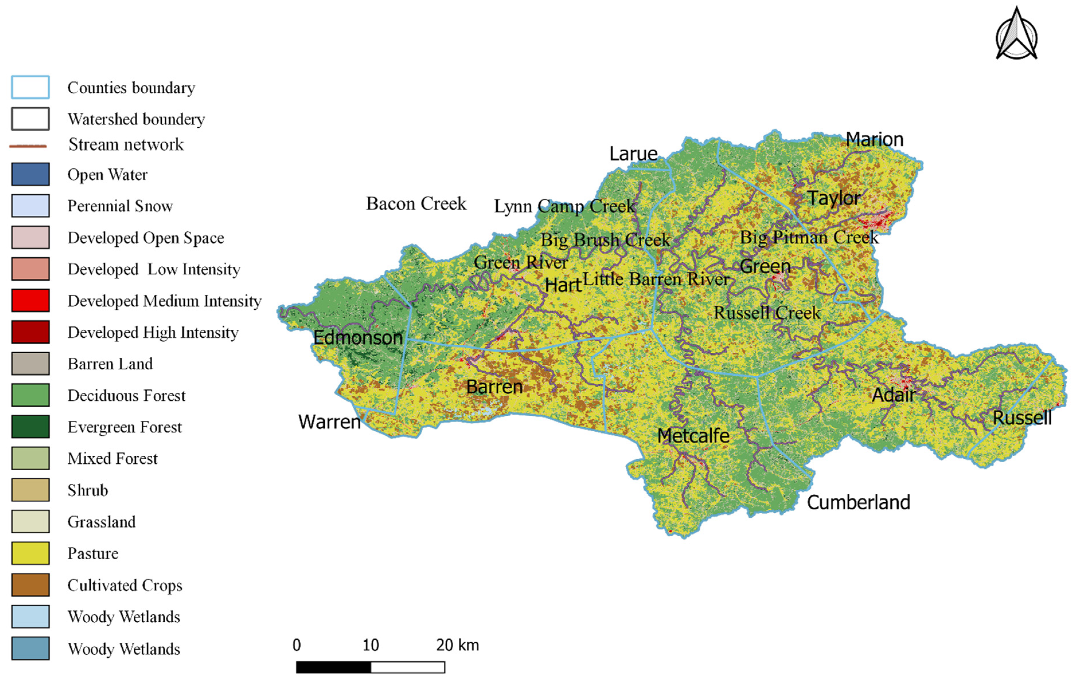
The watershed under study is situated in the lower southwestern part of Kentucky in the USA. The watershed is called the Upper Green River watershed as the main stem of Green River, and its tributaries flow through it. The watershed consists of Russell, Adair, Taylor, Metcalfe, Green, Barren, Hart, and Edmonson counties. Although the watershed contains various land uses such as deciduous, evergreen, mixed forest, transitional, low and high intensity residential, commercial, industrial/transportation, open water, pasture or hay, emergent herbaceous wetlands, row crops, woody wetlands, they can be primarily grouped into three types of land using: urban, forest, and agricultural. The Green River flows through Edmonson, Hart, Green, and Taylor counties and joins the Ohio river downstream of the watershed. Extensive underground karst formations and springs exist between the tributaries of the main stem Green River. The watershed primarily consists of flat-lying limestones, sandstones, and shales forming the karst topography that passes all the surface water through caves and smaller underground passages below the ground surface [28]. The watershed is rated as the fourth most crucial watershed in the United States by the Nature Conservancy and the Natural Heritage Program. It is also the most critical watershed in Kentucky to protect fish and mussel species.
In this watershed, many rural households are not connected to wastewater treatment plants, and the untreated wastewater is directly discharged to streams and creeks, onto overland plains and soils, or into empty spaces of underground. This form of release is known as “straight pipe” discharge. Due to such discharges and failed septic systems, increased fecal coliform bacteria concentrations are found in various portions of the watershed and have essentially impacted the water quality of the Upper Green River basin [28]. The increased concentration of bacteria is so high that the streams are unsafe for fishing, swimming, and body contact. The storage and carefully timed application of animal manure as a fertilizer has been shown to reduce bacteria entering ground water and reduce the need for expensive chemical fertilizers.
2.2. Data
The minimum and maximum elevation levels of the watershed are at 123.14 m and 497.74 m. The minimum and maximum temperatures in a year are around 10.3 °C and 28.9 °C. The average annual precipitation is found to vary between 1041 mm to 1346 mm. The stream water quality sampling stations are located between the latitudes 36.94° and 37.43° and longitudes −86.04° and −85.16°. The water quality data is obtained by measuring samples collected from nearly 42 locations along the Green river monthly from May 2002 to October 2002. The stream network with sampling stations is shown in Figure 1, and the land use map of the watershed is shown in Figure 2. The climate parameters precipitation and temperature are obtained from Kentucky Climate Center. The two-day cumulative precipitation at each sampling location is computed by inverse distance weighted average procedure. The two-day cumulative precipitation, temperature at each sampling station are used along with the land use as inputs into the Decision Tree Classifier model. The six-month period includes a few rainy months and a few non-rainy months.
3. Methodology
3.1. GIS Landuse Analysis
The land use factors developed using GIS analysis [29] essentially indicate the percentage contribution of each land use to the total catchment area or watershed area. The three dominant land use factors are ULUF (urban land use factor), FLUF (forest land use factor), and ALUF (agricultural land use factor). They are given by
Moreover, the above definitions have several advantages as compared to the land uses by simple fractions. The arcsine transformation helps in making the land use distribution near-normal or Gaussian. This transformation gives the values in radians proportional to the angle subtended at the center on a pie chart of land uses [25]. The transformation is known to stabilize the variance and scales the proportional data [30,31,32,33].
3.2. Decision Trees
The decision tree algorithm falls in the category of supervised learning methods [34]. The goal of a decision tree algorithm is to use the appropriate property of the input data (Information Gain, Gain Ratio, or Gini Index) depending on the type of decision tree selected with learning rules to cause splits in the input parameters and give output values as close to the target as possible. Various decision tree models have been devised, which differ in their data splitting methods. Each subsequent model is an improvement over the previous one. A decision tree classifies the input data based on these rules in a top-down fashion. The top node that is assigned all the data is called a root node. The leaf node contains data points that belong to one class or have one specific value, which demarcates the end of a decision tree branch. Further division of the data according to the rules, as mentioned earlier will not be possible. Suppose a node contains heterogeneous data belonging to two or more classes or has two different output values. In that case, that node can be further split to classify data in their respective categories. Such nodes that can be further split are called decision nodes. It is the decision node that takes decisions and propagates the tree to give relevant outputs.
Tree-structured regression methods form a hierarchical structure with the input data being split at the nodes creating smaller subsets till maximum homogeneity is obtained. For example, Y can first be split into and engender two nodes with greater homogeneity than the first node. These two nodes can further be split into {Y | y4 ≥ 27} and {Y | y4 < 27} as shown in Figure 3.
Consequently, similar splitting at each node will result in a tree structure with multiple branches. Selecting a particular attribute and the value of that particular attribute that determines the splitting of data is the basis for nuances in different decision tree models. Classification and Regression Trees (CART), CHAID, ID3, C4.5, and Random Forest are a few to name. For training and testing purposes, the six-month data set covering forty-two locations spread over the stream network is randomly divided into 70% for training and 30% for testing using the scikitlearn library of python programming language. The same training set and testing set are used to examine their classification accuracy for all the decision tree models.
3.3. Attribute Selection Measures
3.3.1. Entropy
Entropy indicates the degree of randomness in a given input set. A branch with 0 entropy is chosen to be the leaf node. If the entropy is not equal to zero, the branch is further split. The Entropy, E(S), measured in “bits” is given by
where pi is the percentage of class i in the node or the probability, and index i runs from 1 to K number of classes or attributes. The process of splitting an attribute is continued until the entropy of resulting subsets is less than the previous input or training set, eventually leading to leaf nodes of zero entropy. Minimization of entropy is desired as it reduces the number of rules of the Decision Trees. The lowering of entropy essentially leads to Decision Trees with fewer branches. The entropy is defined as an information-theoretic measure of the ‘uncertainty’ present in the dataset due to multiple classes [35].
3.3.2. Information Gain
The information gain of an input attribute gives its relation with the target output. A higher information gain suggests that the parameter can separate the training data following the target output to a greater extent. Information gain is inversely proportional to the entropy. The higher the randomness in a set of inputs, the lower will be the information gain. The ID3 model [36] uses Information Gain as the method for classification.
where the index j runs from 1 to K possible classes. Maximizing the information gain essentially leads to minimization of entropy for that particular attribute. In the above Equation (5), the first term on the right-hand side is fixed or it is the entropy at the beginning. The attribute is selected for splitting first for which we obtain the minimal second term on the right-hand side resulting in maximization of information gain for that particular attribute.
3.3.3. Gini Index
It is obtained by the sum of squares of individual probabilities of each class from one. A Higher Gini index value indicates higher homogeneity. The CART algorithm uses the Gini Index to create splits in data [37]. The equation gives Gini index at a node
where pi is the percentage of class i in the node, and the index i runs from 1 to K number of classes. It measures the “impurity” of a dataset. It takes a minimal value of zero to a maximal value of (1-1/K). In the attribute selection process of Decision Tree modeling, that particular attribute is selected for which there is a largest reduction in the value of Gini index. It turns out the reduction of Gini index essentially is accompanied by lowering of entropy.
3.3.4. Gain Ratio
C4.5, an improvised version of ID3, uses gain ratio to create splits in the input data. The Gain ratio removes the bias that exists in calculating the information gain of an input parameter. Information gain prefers the parameter with a large number of input values. To neutralize this, the Gain Ratio divides the Information Gain by the number of branches that would result from the split.
where the index j runs from 1 to K possible number of nonempty classes, and wj is the percentage of class i in the node or the probability. The lower the Split Information, the higher the value of Gain Ratio. The Information Gain is essentially modified by the diversity and distribution of attribute values into the quantity known as Gain Ratio.
3.4. Bagging and Boosting
Bagging, or Bootstrap aggregation, proposed by [38], is a technique used with regression methods to decrease the variance and improve prediction accuracy. It is a simple technique where several bootstrap samples are drawn from the input data, and prediction is made following the same prediction method for each sample. The results are merged by averaging (regression) or simple voting (classification) that adumbrate the input data results subjected to the same prediction method as the bootstrap samples but with reduced variance. All the bootstrap samples have the same size as the original data. The sampling is done with replacement, because of which, a few instances/samples are repeated, and a few are omitted. The stability of base classifier of each bootstrap sample essentially determines the performance of bagging. Since all the samples are equally likely to get aggregated, bagging does not suffer from issues of overfitting and works well with noisy data. Thus, the focus on a specific sample of training data is removed.
Boosting, similar to bagging, is a sample-based approach to improve classification and regression models’ accuracy; however, unlike bagging, which uses a direct averaging of individual sample results, boosting uses a weighted average method to reduce the overall prediction variance. All the samples are initialized with equal weights, then the weights are updated with each boosting classification round. The weights of samples that are harder to classify are increased, and the weights are decreased for the samples that are correctly classified. This ensures the boosting algorithm to focus on samples that are harder to classify with increase in iterations. All the base classifiers of each boosting round are aggregated to obtain the final ensemble boosting classification. The fundamentals of bagging and boosting could be found in [39].
4. Results and Discussion
4.1. Overview
Results obtained using decision trees are discussed in this section. A preliminary statistical analysis is first performed to study the statistics of the experimental data. The results from the initial statistical analysis are given in Table 1.
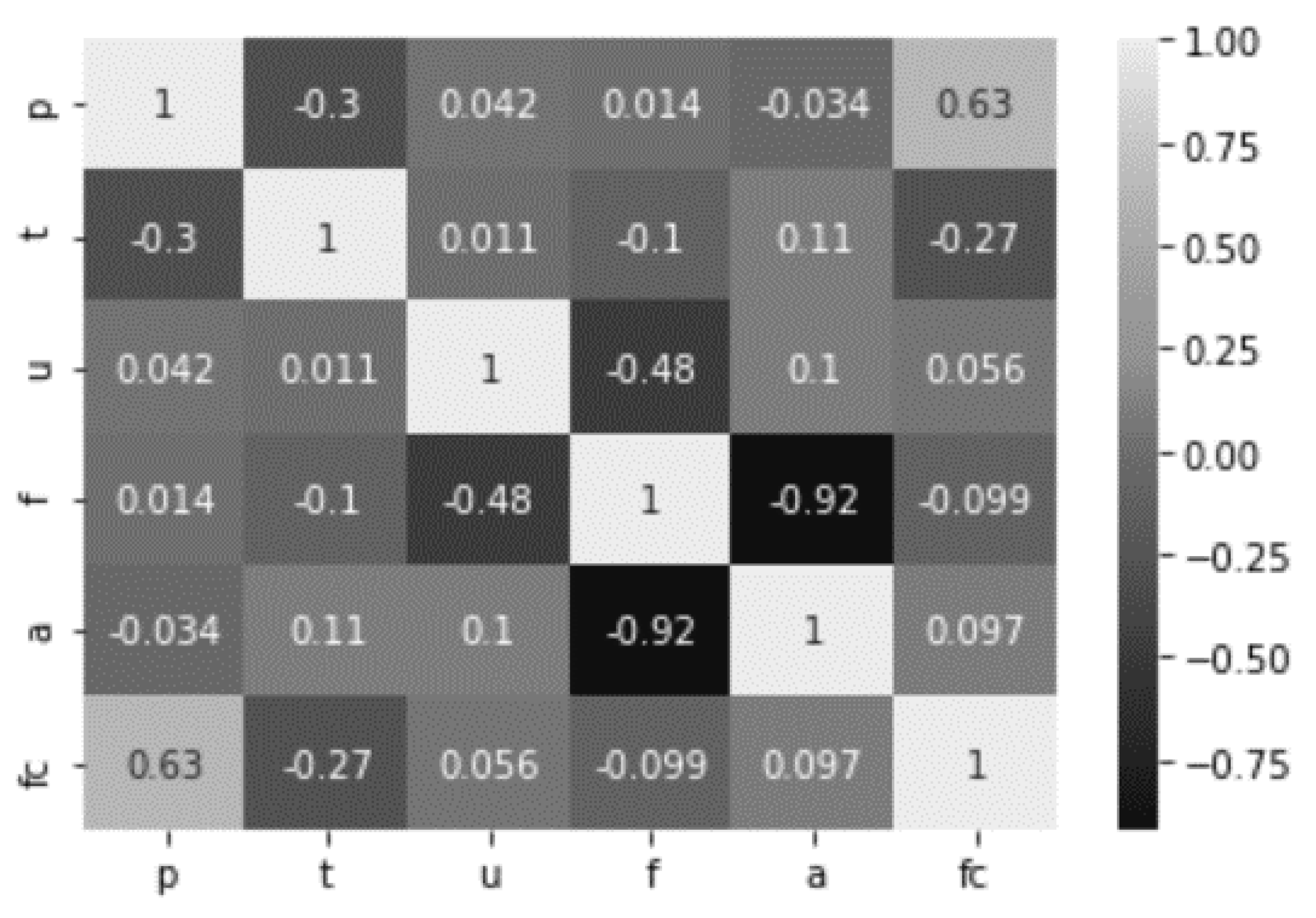
The correlation structure of all the input water sample parameters and the fecal coliform is given by the correlation heatmap shown in Figure 4.
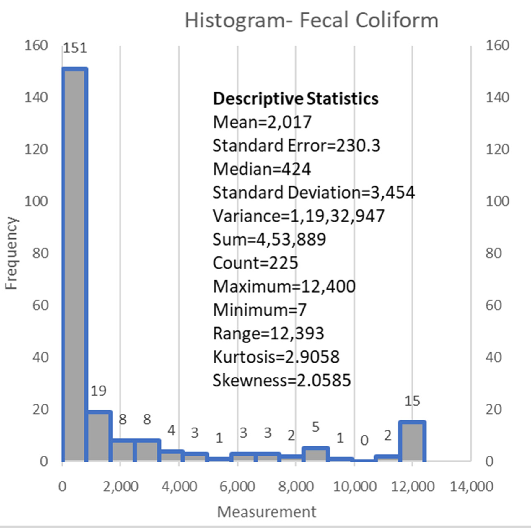
The agriculture land-use factor (ALUF or a) is highly and negatively correlated with the forest land use factor (FLUF or f). FLUF also has a strong negative correlation with urban land use factor (ULUF or u). An exciting inference from the correlation heatmap is the heavy positive correlation between precipitation and fecal coliform (please see Figure 4). A few scatter plots that reveal the relation between the input variables and the fecal coliform individually essentially display the results of the correlation map, i.e., Figure 4, and are not reproduced here. This makes precipitation the most significant variable in determining our output using the decision tree method, and this is evident from the CART and ID3 diagrams given a little later. The precipitation values are obtained at each sampling locations by interpolating the two-day cumulative precipitations at all the gauges in the watershed. The rainfall causes the surface water flow over the watershed’s overland planes consisting of land uses (predominantly urban, forest, and agricultural) and eventually joining the tributaries and mainstem of the Green River. The various parts of the overland planes of the watershed contribute as surface water flows, which enters tributaries first and then the main stem of Green River before reaching the watershed outlet tip. Based on watershed characteristics and time of concentration studies, the two-day cumulative and interpolated precipitation values are most suitable drivers of fecal coliform concentrations than other precipitation measures at all the sampling sites [29]. The positive correlation of microbial indicators such as fecal coliform bacteria and precipitation/rainfall/wet weather conditions is in agreement with the other studies such as that of [40,41,42,43,44] for rivers and bays and [45,46] for lakes. The DTs are best suited for large datasets; however, an attempt is made in the current study because of the multi-dimensional feature space (five independent variables) for monthly instances of data of forty-two locations collected for the six-month period. The DTs are expected to work better for shorter data sets and fewer features as the intrinsic data complexities are reduced. In the present scenario, data limitations on the time frame are offset by the multi-dimensional feature space for varied spatial locations. The reduction of input dimension has been looked into for the same dataset using principal component analysis (PCA), canonical correlation analysis (CCA), and artificial neural networks (ANNs) elsewhere [47]. The authors have found comprehensive predictions using all the spatial parameters such as land uses, and temporal climate parameters. The histogram of fecal coliform is given in Figure 5. The variability of fecal coliform is large as is evident from the high standard deviation and the histogram.
4.2. Results from Decision Tree Models
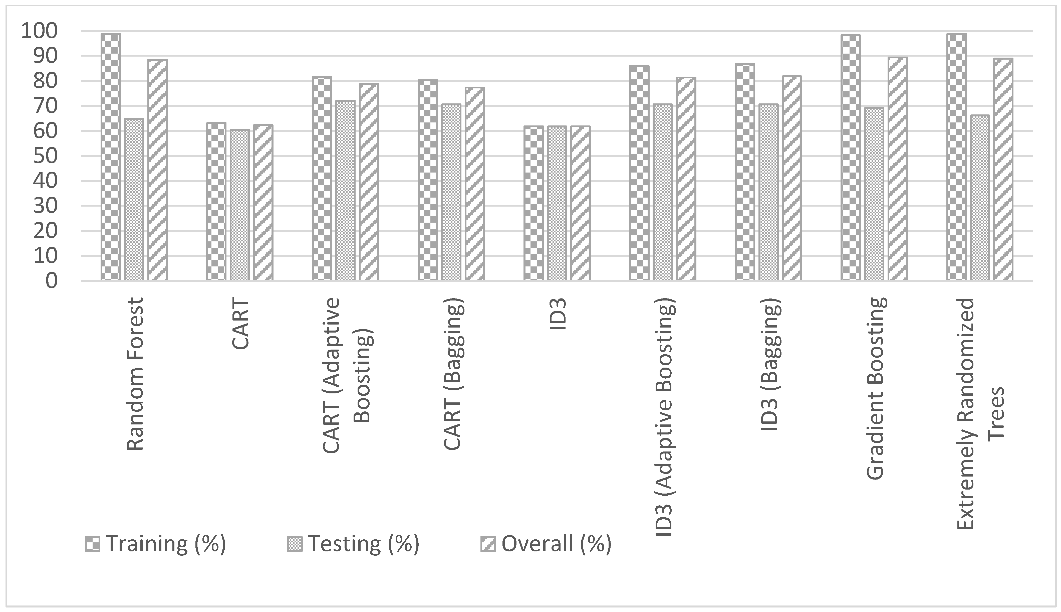
The precipitation, temperature, land use data, and experimentally measured fecal coliform values are used to formulate decision tree models. Several different decision tree models are developed for fecal coliform analysis. All input parameters (precipitation or P, temperature or T, ULUF or u, FLUF or f, ALUF or a) are used to create decision tree models with different data split methods. Precipitation was the single most crucial hydrological input parameter to determine fecal coliform. The correlation values obtained earlier also indicate similar results. 70% of the dataset is used as the training set, and the remaining 30% is used as the testing set. For CART, an accuracy of 63.05% was obtained in the training phase, and 60.29 was obtained in the testing phase. An accuracy of 62.22% was obtained on the entire data set. In CART decision tree modeling, the data is split based on the attribute with the lowest Gini index at the root node in a top-down process with the subsequent splitting of data of attributes of increasing Gini indices till we reach leaf nodes. In this way, the impurity or the uncertainty in the data is minimized with recursive portioning of the data [37]. Similar results were obtained for the ID3 model. Accuracies of 61.78%, 61.76%, and 61.77% were obtained in the training phase, testing phase, and the entire data set, respectively. In the ID3 model, the feature with maximum information gain or smallest entropy is used to split the data at the root node first and then the subsequent nodes till we reach leaf nodes. The least entropy corresponds to the features with the least uncertainty or randomness in the data [36]. Both DTs, CART, and ID3, belong to the family of Top-Down Induction Decision Trees (TDIDT). CART performs slightly better in training than ID3, and ID3 performs slightly better in testing than CART. However, the overall performance of CART is slightly better than ID3. CART and ID3 models were improved by augmenting the simple models with bagging and boosting methods. The highest test set accuracy was obtained for the CART model with adaptive boosting—the accuracy of 81.53%, 72.06%, and 78.67% was obtained in the training phase, testing phase, and entire dataset, respectively. The bagging and adaptive boosting of CART and ID3 perform much better than simple (without bagging and adaptive boosting) CART and ID3 models. Though bagging of ID3 results in largest training accuracy among simple and ensemble models of CART and ID3, the adaptive boosting of CART gives the largest testing accuracy among the same models. However, the overall accuracy of bagging of ID3 model is the highest among simple and ensemble models of CART and ID3 models. Apart from CART and ID3 models, Random Forest was also implemented on the experimental dataset to predict the fecal coliform density or concentration.
The Random Forest model gives an accuracy of 98.7% on the training set, 64.7% on the testing set, and 88.4% on the overall dataset. The Random Forest model is built by creating an ensemble of a large number of decision trees for classification and then predicting the mode or average/mean of all the individual decision tree classification results. The more uncorrelated the individual decision trees are, the better the final prediction or outcome [48]. The individual trees or sub-samples are drawn randomly from the original tree with replacement. The trees are grown to the largest extent possible for classification without pruning of the trees. The features selected in sub-sample trees need to be useful for the effectiveness of the Random Forest model than being pure, random guessing features in classification. The Random forest model outperforms decision trees such as CART, ID3 but its testing accuracy is slightly lower than gradient trees, extremely randomized trees, and DTs with bagging and adaptive boosting. A few other models, such as extremely randomized trees, were also implemented, and the accuracy results of all models are summarized in Table 2 below:
Where ID3-Bagg is ID3 with Bagging, and ID3-AB is ID3 with adaptive boosting. The extremely randomized trees (also known as “Extra Trees”) give a fourth-best testing accuracy of 66.17% and a second-best overall accuracy of 88.89% of all the models. While the Random Forest model uses subsamples with replacement, the extremely randomized trees use the whole input sample. Also, while Random Forest opts for optimum split to select cut points, the extremely randomized trees go for random cut points. The extremely randomized trees are faster and have both features of reducing bias and variance due to usage of original input sample and random split points [49]. Gradient boosting model (GBM) gives third-best testing accuracy of 69.12% and best overall accuracy of 89.33% of all the models. In the Gradient Boosting model, a loss function such as mean square error is minimized with the help of gradient descent principle and an ensemble of weak learners to eventually make correct predictions and become a strong learner tree [50]. The GBM, ERT, and RF perform better than simple and ensemble models of CART, and ID3 in training, and overall accuracies; the ensemble models of CART, and ID3 are slightly better in testing accuracies. This could also be due to possible overtraining of the Decision Tree models in the case of GBM, ERT, and RF. Further, optimal cutting down of trees may result in higher Training, Testing, and Overall accuracies of GBM, ERT, and RF than simple and ensemble models of CART, and ID3. The accuracy of a decision tree model is given by the number of correct predictions made divided by the total number of predictions. Here, the prediction is the class to which the water sample belongs. These results are presented in Figure 6.
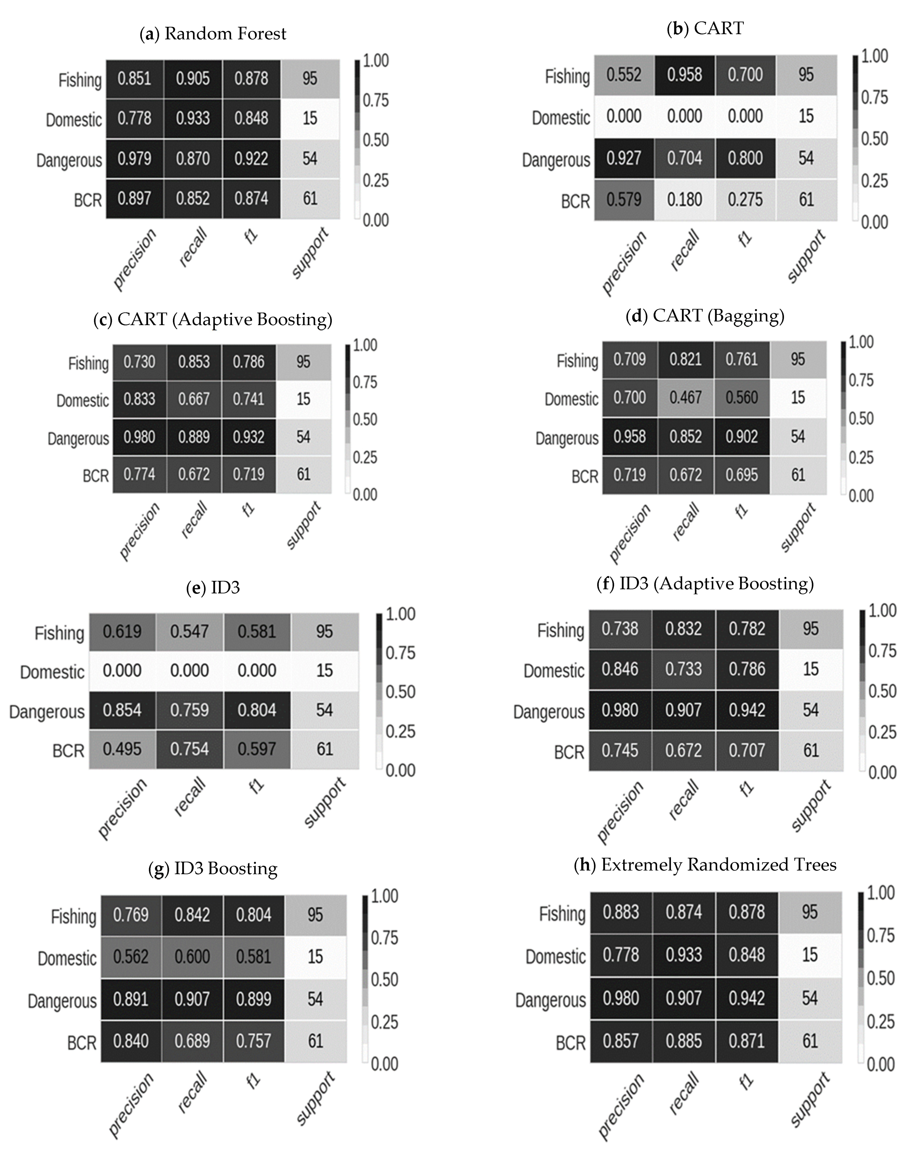
We have used various decision tree algorithms to classify data rather than regression on our current data set. For classification, the target variable, i.e., fecal coliform (FC), was divided into four classes following the United States Environmental Protection Agency (USEPA) recommendations (given in Table 3).
The classified results into four classes or categories, namely- body contact and recreation, fishing and boating, domestic utilization, dangerous for all decision tree algorithms, are presented in Figure 7. The number of samples in each class is also shown in the same Figure. From Figure 6, we can see that high values of precision, recall, and F1-score are obtained for Random Forest, CART with adaptive boosting, ID3 with adaptive boosting, and Extremely randomized trees for the supports shown for all of the four classes. The definitions of accuracy, precision, recall, F1-score are given by:
where TP = True Positive, TN = True Negative, FP = False Positive, FN = False Negative, and support is the number of occurrences of each class in ground truth (correct) target values.
This means that the above four algorithms can correctly classify the positive samples from negative samples for each of the respective class, able to recall all of its positive samples and that both of these abilities are equally important in the classification. Then the best values of precision, recall, and F1-score are obtained for CART with bagging and ID3 with bagging algorithms. Simple CART and ID3 yielded lower precision, recall, and F1-score than the rest of the above algorithms discussed in their respective classifications for each support class. Although not presented here, accuracies were also highest for Extremely randomized trees and Random Forest algorithms, slightly lower for CART and ID3 with bagging and boosting, and lowest for simple CART and ID3 algorithms.
4.3. CART with Bagging and Adaptive Boosting
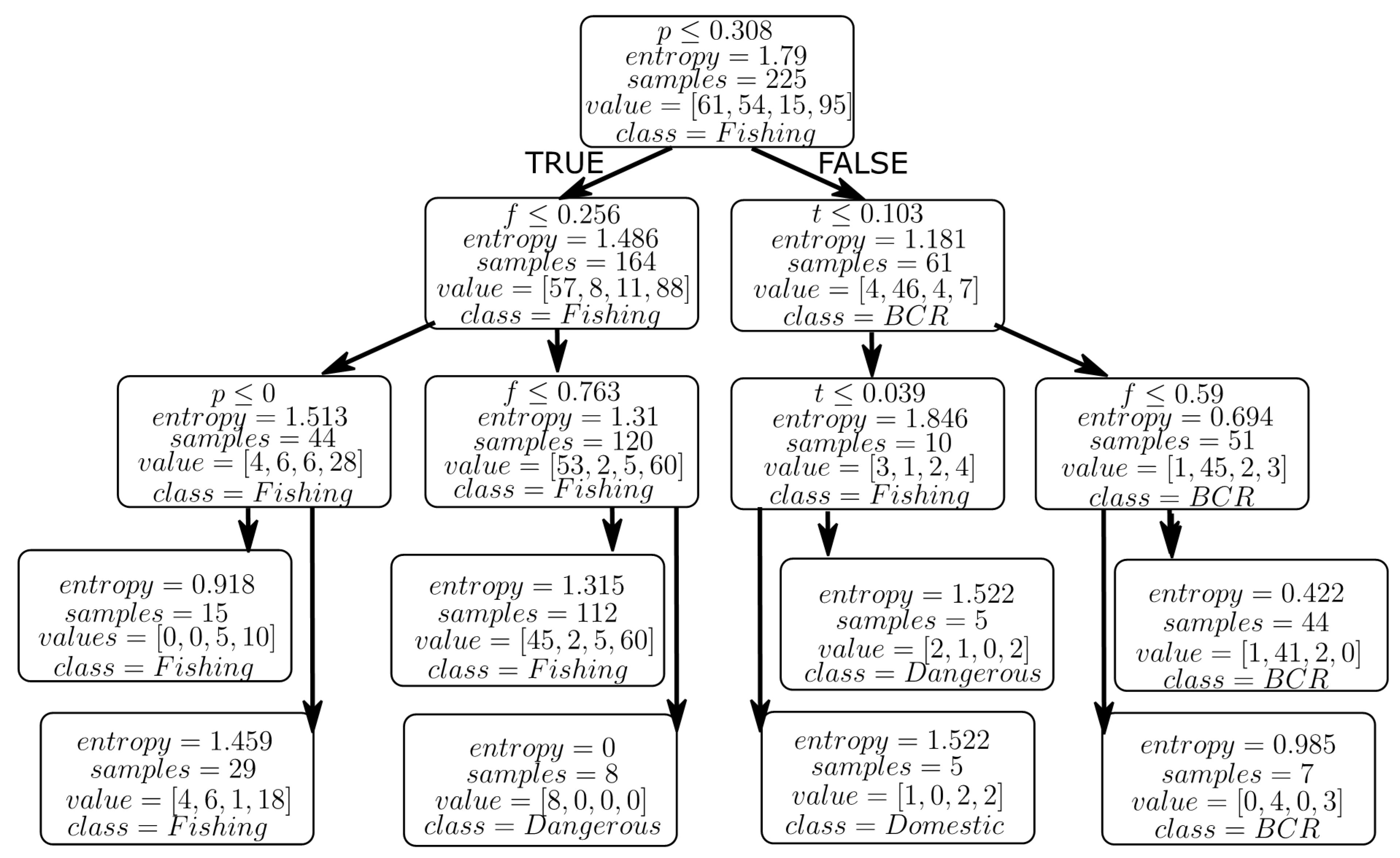
The CART algorithm uses Gini impurity to split data and form a binary classification tree. Implementation of the CART algorithm on our data set results in a tree with four levels (please see Figure 8).
Level 1 has the root node. Level 2 and level 3 contain the decision nodes, and level 4 has the leaf nodes with data split into classes. The tree’s root node containing all 225 data points of our data set has been split based on the precipitation input variable (p) since p is the variable of the highest significance. The decision nodes at level 2 are split using the forest land use factor (f) and the temperature (t) input variables since these nodes represent points of highest Gini impurity. At level 3, we get our first leaf node of class “Dangerous” with eight samples falling in this category (p ≤ 0.308, f ≥ 0.763). The final level contains the leaf nodes that classify the data into the specified classes. The class with the highest number of samples is fishing (156 samples), followed by BCR (51 samples). The classes “Domestic” and “Dangerous” have 5 and 13 samples, respectively, giving us a total of 225 samples in our data set. The CART algorithm is a moderately accurate method to classify our data set, giving an accuracy of 63.05% on the training set and 62.22% on the entire data set. However, improving our model using bagging and boosting methods yield even higher accuracies. From Table 2, CART with adaptive boosting gives the best testing accuracy out of all the decision trees. The adaptive boosting method enables to combine several weak classifiers into a strong classifier through an iterative decision tree modeling. The weak classifiers are weighted highly and trained with a few low-weighted strong classifiers to produce a strong ensemble classifier at the end [51]. From Table 2, we can also see that CART with bagging yields second-best testing accuracy. Bagging simply means “bootstrap aggregating.” The implementation of CART with bagging results in creating many random sub-samples with replacement and training CART model on each sample. Then the average prediction is made on all the samples [38]. We can see that the ensemble predictions of bagging and boosting of the CART model are better than the simple CART model results.
4.4. ID3 with Bagging and Adaptive Boosting
Like the CART algorithm that uses Gini impurity to form splits in the data set, the ID3 decision tree utilizes the information gain and entropy. Implementation of the ID3 algorithm on our data set also yields a tree with four levels (please see Figure 9).
Again, since “p” is the most significant variable, the root node is split using the “Precipitation” input variable. The decision nodes in level 3 and level 4 are split to maintain lower Information Gain and Entropy uncertainty. Level 4 of the ID3 decision tree has the dataset classified into four pre-defined classes. Similar to the CART algorithm results, the class with the highest number of samples is “Fishing” followed by “BCR,” “Dangerous” and “Domestic.” The accuracies obtained for the training data set and overall dataset are 61.78% and 61.77% respectively, which is slightly lower than that obtained by the CART algorithm. From Table 2, we can see that ID3 with adaptive boosting comparable results to that of CART with adaptive boosting. Adaboost is an iterative procedure with no replacement. It generates a strong ensemble classifier by putting high weights on the mis-classifiers and low weights on the correctly classified trees to reduce bias and variance in the model. For this reason, it is called the “best out-of-the-box classifier” usually. The second-best testing accuracy is obtained using this method with ID3 in all attempted decision tree models. ID3 with bagging results can also be seen from Table 2, which creates many independent bootstrap aggregation models and associates weak learner with each model to finally aggregate them to produce average or ensemble prediction that has a lower variance. This method also yields the second best testing accuracy of all the decision tree models. We can see that the bagging and boosting ensemble methods improve the testing accuracy compared to simple ID3.
4.5. Decision Tree Classifier Based Decision Support System (DTCDSS)
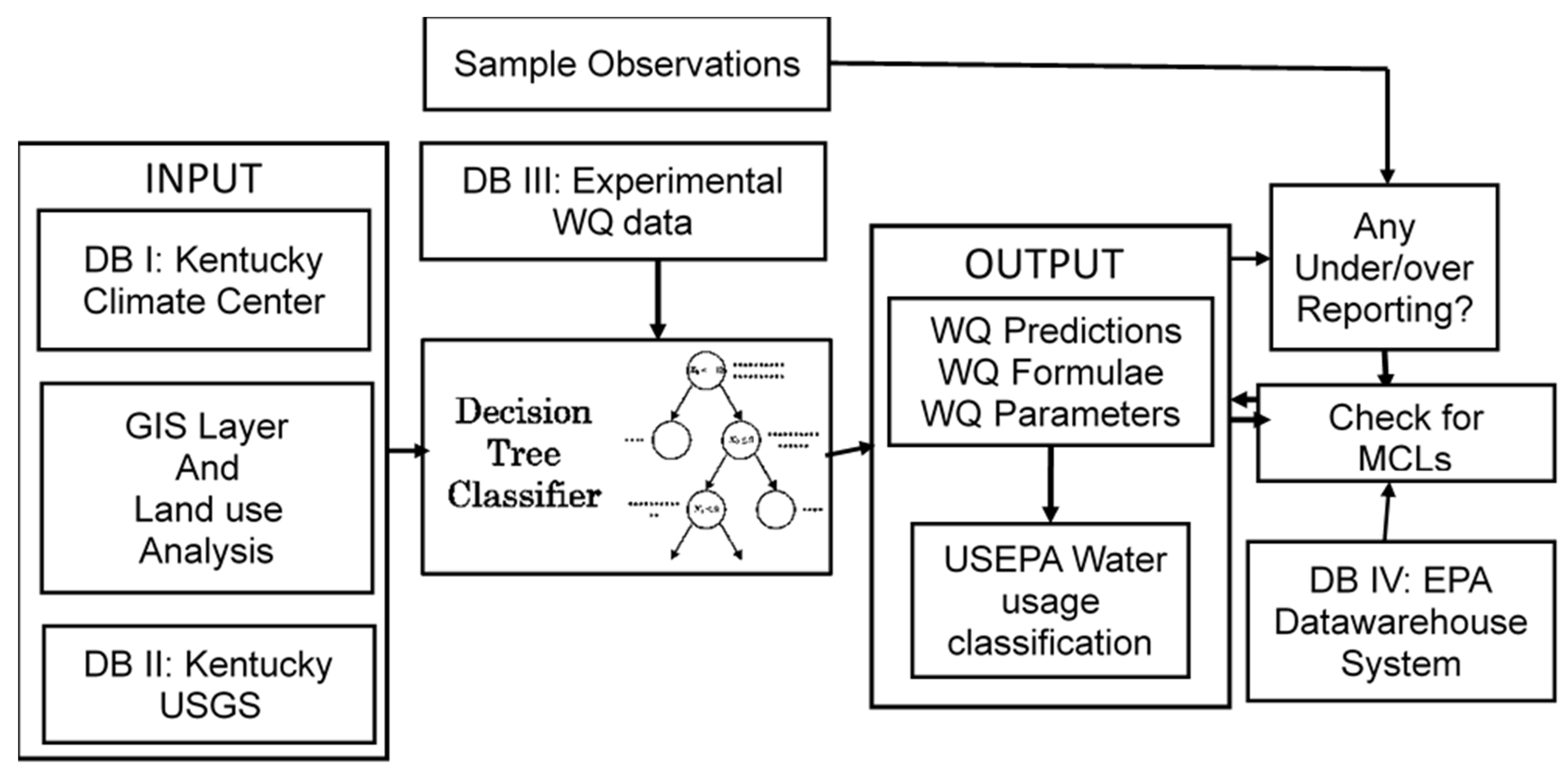
A Decision Support System (DSS) can be built from the above results of decision tree models, as shown in Figure 10.
The input parameters and the sample water quality observations come from the input databases, as shown in the decision tree classifier (DTC). The above-discussed decision tree models help classify the water quality data based on input parameters and respective decision tree algorithms. The results are shown in the output database in “water quality predictions/formulae/bounds”. The outputs are put into and as per classes of US EPA water usage classification. From the output classifications, one could figure out the under/over reporting issues, and check for maximum contamination levels (MCLs). In this process, the US EPA data warehouse system will help compare the output water quality parameters with stipulated MCLs. The inner working of any of the above-discussed decision tree classifiers is shown in the flow chart Figure 11.
Firstly, the DTC classifier receives the input data from the input databases such as climate, land use data, and water quality data. The entropy or information gain, gain ratio, and Gini index are computed based on the particular model chosen of the decision tree in the DTC classifier. For example, if the decision tree in the DTC classifier is ID3, then entropy or information gain is computed. If the decision tree in the DTC classifier is CART, then the gain ratio is computed. Similarly, if the decision tree is C4.5, then the Gini index is computed. The input parameters and the output parameters of a data sample are presented at the root node first. Then the tree is split based on the decision of the “if-else” statement minimizing the heterogeneity of data or increasing the homogeneity. The tree branches keep increasing with the addition of new data samples at the root node, and slowly, the leaf nodes get formed. At every level node of the tree, the entropy or information gain, gain ratio, Gini index are computed so that the data could be split easily and the data get traversed to the leaf nodes. Thus, the DTC classifier helps us classify the data or make a decision into four classes of output, namely, body contact and recreation, fishing and boating, domestic utilization, and dangerous at the leaf nodes. The model performance can be computed using the metrics such as accuracy, precision, recall, and F1-score. The particular DT model in the classifier can be any one of the CART, ID3, C4.5 with bagging and boosting variants, Random Forest, and Extremely Randomized Trees. The output performance of the DSS can be specific to the DT model chosen and could also be data sensitive. The best DT model for the DSS can be fixed only by experimenting with above-stated decision tree models for the data of several watersheds consisting of stream networks of varied conditions. Suppose we replace the DTC classifier with Decsion Tree Regressor (DTR). In that case, we will be able to predict the output parameter such as fecal coliform, from the input parameters such as climate and land use. The output parameter predictions can also be further generalized or recasted using the regression formulae obtained of DTR and the output parameter bounds. The current Decision Support System is an improvised version of the DSS discussed in [29]. The Artificial Neural Network (ANN) model is replaced by DTC to suit the current problem of classification stream waters into four classes. The performances of DSS using DTR, the comparison of DTR and ANN models are out of the scope of the current work and are pursued elsewhere as separate research studies. Comparing output parameter predictions with respective MCLs within the DSS framework ensures the suitability of stream waters broadly into “safe” or “unsafe,” thus making a helpful decision.
5. Conclusions
The classification abilities of Decision Trees such as CART, ID3, RF, and ensemble methods such as bagging and boosting are utilized for the classification and prediction of Fecal Coliform (FC) into four classes in this study. The variable with maximum information gain and gain ratio in the case of ID3 model, and the variable with maximum Gini Index in the case of CART model are selected at the root node, and such criteria used further down the tree till the leaf nodes, using DT algorithms for best classification in terms of maximum accuracy. The algorithms perform comparably well with each other, Random Forests being the most consistent in the classification of Fecal Coliform for the Upper Green River watershed overall. It performs better than CART and ID3 in all the phases, i.e., training, testing, and overall. Gradient Boosting and Extremely Randomized Trees are the other DT algorithms that show comparable accuracies as that of Random Forest in training and testing phases. The CART decision tree with Adaptive Boosting yielded the best testing accuracy. In contrast, the CART with Bagging and ID3 with Bagging and Adaptive Boosting yielded the comparable second-best testing accuracies respectively out of all the decision tree modeling attempts. There is no proof of exactly the same feature or attribute will be chosen for each node of the resulting tree for various DT algorithms. There is also no guarantee that accuracy of classification will be higher for the proposed classifier as it needs to be tested for a variety of water quality parameters of different watersheds under climate changes. Also, being greedy at each step/node may not ensure overall minimization of entropy or global optimization of the classification process. In the present work, the authors have focused on only the classification capabilities of the Decision Trees for this particular watershed/dataset. The present work explores the classification capabilities in training and testing phases only. The size of the data was one limitation because of which, the authors could not go for cross-validation. However, the depth of the successful trees is essentially governed by maximizing the information gain or minimizing the entropy, i.e., randomness at every level. It is generally found that the shorter trees are prone to better classification capabilities than the more extended trees [52] (Mitchell, 1997). This is due to lesser overtraining of the trees, leading to more successful generalization or predictions. From the above discussion of results, the following salient conclusions can be made as follows:
- (i)
- The Decision Trees of Gradient Boosting (GB), Extremely Randomized Trees (ERT), and RF perform better than simple (without bagging and boosting) ID3, and CART models in training, testing, and overall.
- (ii)
- The bagging and adaptive boosting Decision Trees of CART, and ID3 significantly improve the performance over simple (without bagging and boosting) CART, and ID3 models.
- (iii)
- The performances of bagging and adaptive boosting Decision Trees of CART, and ID3 are slightly better than GB, ERT, and RF in testing. However, the training and overall accuracies of GB, ERT, and RF are better than all the models (including bagging and adaptive boosting) of CART and ID3.
- (iv)
- The Decision Tree models of GB, ERT, and RF are more consistent than other models in training, testing, and overall accuracies.
- (v)
- Overtraining the trees increases training accuracy at the expense of testing accuracy. A judicious choice need to be made in cutting down the trees, so that an optimal performance of training, testing, and overall accuracies is obtained.
Author Contributions
A.H.—Methodology, software, validation, writing-original draft preparation, visualization; J.A.—Conceptualization, methodology, validation, writing-review and editing, visualization, validation, software, formal analysis, investigation, supervision, project administration, funding acquisition; All authors have read and agreed to the published version of the manuscript.
Funding
Council of Scientific and Industrial Research (CSIR), India grant (No. 24 (0356)/19/EMR-II), project titled “Experimental and Computational studies of Surface Water Quality parameters from Morphometry and Spectral Characteristics”.
Institutional Review Board Statement
Not applicable.
Informed Consent Statement
Not applicable.
Data Availability Statement
The data is owned by Upper Green Biological Preserve, Department of Biology, Western Kentucky University, Bowling Green, Kentucky, USA.
Acknowledgments
The corresponding author would like to express acknowledgments to the Council of Scientific and Industrial Research (CSIR), India grant (No. 24 (0356)/19/EMR-II) of the project titled “Experimental and Computational studies of Surface Water Quality parameters from Morphometry and Spectral Characteristics.” The authors would like to thank Ouida Meier, Albert Meier, Stuart Foster, Tim Rink, and Jenna Harbaugh for providing us with the required data. The authors would like to thank Vamsi Krishna Sridharan, Institute of Marine Sciences, University of California, Santa Cruz, California, USA for a detailed review and comments of the manuscript. The authors would also like to thank M.M. Prakash Mohan and N.Satish, Research Scholars, Department of Civil Engineering, Birla Institute of Technology and Science, Pilani, Hyderabad Campus for helping out with a couple of figures.
Conflicts of Interest
The authors declare no conflict of interest.
References
- Ormsbee, L.J.; Anmala, S.E.M. Total Maximum Daily Load (TMDL) Development for Eagle Creek; Report submitted to Kentucky Department for Environmental Protection, Division of Water, Frankfort; University of Kentucky: Lexington, Kentucky, 2002. [Google Scholar]
- D’Agostino, V.; Greene, E.A.; Passarella, G.; Vurro, M. Spatial and temporal study of nitrate concentration in groundwater by means of coregionalization. Environ. Earth Sci. 1998, 36, 285–295. [Google Scholar] [CrossRef]
- Gaus, I.; Kinniburgh, D.G.; Talbot, J.C.; Webster, R. Geostatistical analysis of arsenic concentration in groundwater in Bangladesh using disjunctive kriging. Environ. Earth Sci. 2003, 44, 939–948. [Google Scholar] [CrossRef] [Green Version]
- Arslan, H. Spatial and temporal mapping of groundwater salinity using ordinary kriging and indicator kriging: The case of Bafra Plain, Turkey. Agric. Water Manag. 2012, 113, 57–63. [Google Scholar] [CrossRef]
- Ahn, H.; Chon, H. Assessment of groundwater contamination using geographic information systems. Environ. Geochem. Health 1999, 21, 273–289. [Google Scholar] [CrossRef]
- Bae, H.-K.; Olson, B.H.; Hsu, K.-L.; Sorooshian, S. Classification and regression tree (CART) analysis for indicator bacterial concentration prediction for a Californian coastal area. Water Sci. Technol. 2010, 61, 545–553. [Google Scholar] [CrossRef]
- Liao, H.; Sun, W. Forecasting and Evaluating Water Quality of Chao Lake based on an Improved Decision Tree Method. Procedia Environ. Sci. 2010, 2, 970–979. [Google Scholar] [CrossRef] [Green Version]
- Nikoo, M.R.; Karimi, A.; Kerachian, R.; Poorsepahy-Samian, H.; Daneshmand, F. Rules for Optimal Operation of Reservoir-River-Groundwater Systems Considering Water Quality Targets: Application of M5P Model. Water Resour. Manag. 2013, 27, 2771–2784. [Google Scholar] [CrossRef]
- Azam, M.; Aslam, M.; Khan, K.; Mughal, A.; Inayat, A. Comparisons of decision tree methods using water data. Commun. Stat. -Simul. Comput. 2016, 46, 2924–2934. [Google Scholar] [CrossRef]
- Maier, P.M.; Keller, S. Machine Learning Regression on Hyperspectral Data to Estimate Multiple Water Parameters. In 2018 9th Workshop on Hyperspectral Image and Signal Processing: Evolution in Remote Sensing (WHISPERS); IEEE: Piscataway, NJ, USA, 2018; pp. 1–5. [Google Scholar]
- Jerves-Cobo, R.; Córdova-Vela, G.; Iñiguez-Vela, X.; Díaz-Granda, C.; Van Echelpoel, W.; Cisneros, F.; Nopens, I.; Goethals, P.L.M. Model-Based Analysis of the Potential of Macroinvertebrates as Indicators for Microbial Pathogens in Rivers. Water 2018, 10, 375. [Google Scholar] [CrossRef] [Green Version]
- Geetha Jenifel, M.; Jemila Rose, R. Recursive partitioning algorithm in water quality prediction. Int. J. Environ. Sci. Technol. 2020, 17, 745–754. [Google Scholar] [CrossRef]
- Ho, J.Y.; Afan, H.A.; El-Shafie, A.H.; Koting, S.B.; Mohd, N.S.; Jaafar, W.Z.B.; Sai, H.L.; Malek, M.A.; Ahmed, A.N.; Mohtar, W.H.M.W.; et al. Towards a time and cost effective approach to water quality index class prediction. J. Hydrol. 2019, 575, 148–165. [Google Scholar] [CrossRef]
- Sepahvand, A.; Singh, B.; Sihag, P.; Samani, A.N.; Ahmadi, H.; Nia, S.F. Assessment of the various soft computing techniques to predict sodium absorption ratio (SAR). ISH J. Hydraul. Eng. 2019, 1–12. [Google Scholar] [CrossRef]
- Lu, H.; Ma, X. Hybrid decision tree-based machine learning models for short-term water quality prediction. Chemosphere 2020, 249, 126169. [Google Scholar] [CrossRef]
- Shin, Y.; Kim, T.; Hong, S.; Lee, S.; Lee, E.; Hong, S.; Lee, C.; Kim, T.; Park, M.S.; Park, J.; et al. Prediction of Chlorophyll-a Concentrations in the Nakdong River Using Machine Learning Methods. Water 2020, 12, 1822. [Google Scholar] [CrossRef]
- Mosavi, A.; Hosseini, F.S.; Choubin, B.; Abdolshahnejad, M.; Gharechaee, H.; Lahijanzadeh, A.; Dineva, A.A. Susceptibility Prediction of Groundwater Hardness Using Ensemble Machine Learning Models. Water 2020, 12, 2770. [Google Scholar] [CrossRef]
- Naloufi, M.; Lucas, F.S.; Souihi, S.; Servais, P.; Janne, A.; De Abreu, T.W.M. Evaluating the Performance of Machine Learning Approaches to Predict the Microbial Quality of Surface Waters and to Optimize the Sampling Effort. Water 2021, 13, 2457. [Google Scholar] [CrossRef]
- Chen, K.; Chen, H.; Zhou, C.; Huang, Y.; Qi, X.; Shen, R.; Liu, F.; Zuo, M.; Zou, X.; Wang, J.; et al. Comparative analysis of surface water quality prediction performance and identification of key water parameters using different machine learning models based on big data. Water Res. 2020, 171, 115454. [Google Scholar] [CrossRef]
- Alizamir, M.; Heddam, S.; Kim, S.; Mehr, A.D. On the implementation of a novel data-intelligence model based on extreme learning machine optimized by bat algorithm for estimating daily chlorophyll-a concentration: Case studies of river and lake in USA. J. Clean. Prod. 2021, 285, 124868. [Google Scholar] [CrossRef]
- Khullar, S.; Singh, N. Machine learning techniques in river water quality modelling: A research travelogue. Water Supply 2021, 21, 1–13. [Google Scholar] [CrossRef]
- Asadollah, S.B.H.S.; Sharafati, A.; Motta, D.; Yaseen, Z.M. River water quality index prediction and uncertainty analysis: A comparative study of machine learning models. J. Environ. Chem. Eng. 2021, 9, 104599. [Google Scholar] [CrossRef]
- Zounemat-Kermani, M.; Alizamir, M.; Fadaee, M.; Namboothiri, A.S.; Shiri, J. Online sequential extreme learning machine in river water quality (turbidity) prediction: A comparative study on different data mining approaches. Water Environ. J. 2021, 35, 335–348. [Google Scholar] [CrossRef]
- Bui, D.T.; Khosravi, K.; Tiefenbacher, J.; Nguyen, H.; Kazakis, N. Improving prediction of water quality indices using novel hybrid machine-learning algorithms. Sci. Total. Environ. 2020, 721, 137612. [Google Scholar] [CrossRef]
- Jeihouni, M.; Toomanian, A.; Mansourian, A. Decision Tree-Based Data Mining and Rule Induction for Identifying High Quality Groundwater Zones to Water Supply Management: A Novel Hybrid Use of Data Mining and GIS. Water Resour. Manag. 2020, 34, 139–154. [Google Scholar] [CrossRef] [Green Version]
- Saghebian, S.M.; Sattari, M.T.; Mirabbasi, R.; Pal, M. Ground water quality classification by decision tree method in Ardebil region, Iran. Arab. J. Geosci. 2014, 7, 4767–4777. [Google Scholar] [CrossRef]
- Anmala, J.; Turuganti, V. Comparison of the performance of decision tree (DT) algorithms and extreme learning machine (ELM) model in the prediction of water quality of the Upper Green River watershed. Water Environ. Res. 2021. [Google Scholar] [CrossRef] [PubMed]
- Status Report, Green and Tradewater Basins; Kentucky Division of Water: Frankfort, KY, USA, 2001.
- Anmala, J.; Meier, O.W.; Meier, A.J.; Grubbs, S. A GIS and an artificial neural network based water quality model for a stream network in Upper Green River Basin, Kentucky, USA. ASCE J. Environm. Eng. 2015, 141, 04014082. [Google Scholar] [CrossRef]
- Kaplan, C.; Pasternack, B.; Shah, H.; Gallo, G. Age-related incidence of sclerotic glomeruli in human kidneys. Am. J. Pathol. 1975, 80, 227–234. [Google Scholar]
- Sokal, R.R.; Rohlf, J.F. Biometry: The Principle and Practice of Statistics in Biological Research, 2nd ed.; W.H. Freeman and Company: San Francisco, CA, USA, 1981. [Google Scholar]
- Snedecor, G.W.; Cochran, W.G. Statistical Methods, 8th ed.; Iowa University Press: Ames, IA, USA, 1989. [Google Scholar] [CrossRef]
- Rao, P.V. Statistical Research Methods in the Life Sciences; Duxbury Press: Austin, TX, USA, 1998; 889p. [Google Scholar]
- Sutton, C.D. Classification and Regression Trees, Bagging, and Boosting. Hand. Stat. 2005, 24, 303–329. [Google Scholar] [CrossRef] [Green Version]
- Bramer, M. Principles of Data Mining; Springer: London, UK, 2007; 343p, ISBN 978-1-84628-765-7. [Google Scholar]
- Quinlan, J.R. Induction of Decision Trees. Mach. Learn. 1986, 1, 81–106. [Google Scholar] [CrossRef] [Green Version]
- Breiman, L.; Firedman, J.H.; Olshen, R.A.; Stone, C.J. Classification and Regression Trees; Chapman & Hall/CRC: Boca Raton, FL, USA, 1984; ISBN 978-0-412-04841-8. [Google Scholar]
- Breiman, L. Bagging predictors. Mach. Learn. 1996, 24, 123–140. [Google Scholar] [CrossRef] [Green Version]
- Tan, P.-N.; Steinbach, M. Introduction to Data Mining; Pearson India Education Services Pvt. Ltd: Bengaluru, India, 2016; p. 760. [Google Scholar]
- Shehane, S.; Harwood, V.; Whitlock, J.; Rose, J. The influence of rainfall on the incidence of microbial faecal indicators and the dominant sources of faecal pollution in a Florida river. J. Appl. Microbiol. 2005, 98, 1127–1136. [Google Scholar] [CrossRef]
- Santiago-Rodriguez, T.M.; Tremblay, R.L.; Toledo-Hernandez, C.; Gonzalez-Nieves, J.E.; Ryu, H.; Domingo, J.W.S.; Toranzos, G.A. Microbial Quality of Tropical Inland Waters and Effects of Rainfall Events. Appl. Environ. Microbiol. 2012, 78, 5160–5169. [Google Scholar] [CrossRef] [Green Version]
- Islam, M.M.M.; Hofstra, N.; Islam, A. The Impact of Environmental Variables on Faecal Indicator Bacteria in the Betna River Basin, Bangladesh. Environ. Process. 2017, 4, 319–332. [Google Scholar] [CrossRef]
- Leight, A.K.; Crump, B.C.; Hood, R. Assessment of Fecal Indicator Bacteria and Potential Pathogen Co-Occurrence at a Shellfish Growing Area. Front. Microbiol. 2018, 9, 384. [Google Scholar] [CrossRef] [Green Version]
- Seo, M.; Lee, H.; Kim, Y. Relationship between Coliform Bacteria and Water Quality Factors at Weir Stations in the Nakdong River, South Korea. Water 2019, 11, 1171. [Google Scholar] [CrossRef] [Green Version]
- Kagalou, I.; Tsimarakis, G.; Bezirtzoglou, E. Inter-relationships between Bacteriological and Chemical Variations in Lake Pamvotis—Greece. Microb. Ecol. Health Dis. 2002, 14, 37–41. [Google Scholar] [CrossRef] [Green Version]
- Jin, G.; Englande, A.; Bradford, H.; Jeng, H.-W. Comparison of E.Coli, Enterococci, and Fecal Coliform as Indicators for Brackish Water Quality Assessment. Water Environ. Res. 2004, 76, 245–255. [Google Scholar] [CrossRef] [PubMed]
- Venkateswarlu, T.; Anmala, J.; Dharwa, M. PCA, CCA, and ANN modeling of climate and land-use effects on stream water quality of Karst watershed in Upper Green River, Kentucky, USA. ASCE J. Hydrol. Eng. 2020, 25, 05020008. [Google Scholar] [CrossRef]
- Breiman, L. Random forests. Mach. Learn. 2001, 45, 5–32. [Google Scholar] [CrossRef] [Green Version]
- Geurts, P.; Ernst, D.; Wehenkel, L. Extremely randomized trees. Mach. Learn. 2006, 63, 3–42. [Google Scholar] [CrossRef] [Green Version]
- Breiman, L. Arcing the Edge; Technical Report 486, Ann. Prob; Statistics Department, University of California: Berkeley, CA, USA, 1997; Volume 26, pp. 1683–1702. [Google Scholar]
- Freund, Y.; Schapire, R.E. A short introduction to Boosting. J. Jpn. Soc. Artif. Intell. 1999, 14, 771–780. [Google Scholar]
- Mitchell, T.M. Machine Learning, 1st ed.; Mc-Graw Hill Education: New York, NY, USA, 1997. [Google Scholar]
Figure 1.
The stream networkand the sampling stations in the Upper Green River watershed.

Figure 2.
Land Use Map of Upper Green River Watershed.

Figure 3.
A simple tree at classification.

Figure 4.
Correlation Heatmap.

Figure 5.
Histogram of Fecal Coliform (FC).

Figure 6.
Bar graph of training, testing, and overall accuracies of different DT models.

Figure 7.
Classification reports of the entire dataset using different DT models.

Figure 8.
The Decision Tree developed using the CART algorithm.

Figure 9.
The Decision Tree developed using the ID3 algorithm.

Figure 10.
Decision Tree Classifier based Decision Support System (DTCDSS).

Figure 11.
Flow Chart of a Decision Tree Classifier Model.


Table 1.
Statistics of Water Quality Parameter and inputs.
| Water Quality Parameter | Variable | Sum | Average | Standard Deviation | Input/Output |
|---|---|---|---|---|---|
| Precipitation (in cm) | P | 817.0 | 3.6 | 4.21 | Input |
| Temperature (°C) | T | 4250.7 | 18.9 | 4.36 | Input |
| Urban land-use factor | U | 35.3 | 0.16 | 0.12 | Input |
| Forest land-use factor | F | 165.2 | 0.73 | 0.12 | Input |
| Agricultural land-use factor | A | 178.0 | 0.79 | 0.11 | Input |
| Fecal Coliform (#colonies/100 mL) | FC | 453,889 | 2017.3 | 3454 | Output |
Table 2.
Accuracies of various DT models in the prediction of FC.
| Model | Training (%) | Testing (%) | Overall (%) |
|---|---|---|---|
| CART (Adaptive Boosting) | 81.53 | 72.06 | 78.67 |
| ID3-Bagg | 86.62 | 70.58 | 81.78 |
| ID3-AB | 85.98 | 70.58 | 81.33 |
| CART (Bagging) | 80.25 | 70.58 | 77.33 |
| Gradient Boosting (GBM) | 98.19 | 69.12 | 89.33 |
| Extremely Randomized Trees (ERT) | 98.72 | 66.17 | 88.89 |
| Random Forest (RF) | 98.70 | 64.70 | 88.40 |
| ID3 | 61.78 | 61.76 | 61.77 |
| CART | 63.05 | 60.29 | 62.22 |
Table 3.
Fecal Coliform and its Class.
| Class | Fecal Coliform (FC) Range (cfu/100 mL) |
|---|---|
| Body contact and recreation (BCR) | 0 < FC ≤ 200 |
| Fishing and boating | 200 < FC ≤ 1000 |
| Domestic utilization | 1000 < FC ≤ 2000 |
| Dangerous | FC > 2000 |
Publisher’s Note: MDPI stays neutral with regard to jurisdictional claims in published maps and institutional affiliations. |
© 2021 by the authors. Licensee MDPI, Basel, Switzerland. This article is an open access article distributed under the terms and conditions of the Creative Commons Attribution (CC BY) license (https://creativecommons.org/licenses/by/4.0/).
Share and Cite
MDPI and ACS Style
Hannan, A.; Anmala, J. Classification and Prediction of Fecal Coliform in Stream Waters Using Decision Trees (DTs) for Upper Green River Watershed, Kentucky, USA. Water 2021, 13, 2790. https://0-doi-org.brum.beds.ac.uk/10.3390/w13192790
AMA Style
Hannan A, Anmala J. Classification and Prediction of Fecal Coliform in Stream Waters Using Decision Trees (DTs) for Upper Green River Watershed, Kentucky, USA. Water. 2021; 13(19):2790. https://0-doi-org.brum.beds.ac.uk/10.3390/w13192790
Chicago/Turabian StyleHannan, Abdul, and Jagadeesh Anmala. 2021. "Classification and Prediction of Fecal Coliform in Stream Waters Using Decision Trees (DTs) for Upper Green River Watershed, Kentucky, USA" Water 13, no. 19: 2790. https://0-doi-org.brum.beds.ac.uk/10.3390/w13192790
Note that from the first issue of 2016, this journal uses article numbers instead of page numbers. See further details here.