Aquatic Biological Diversity Responses to Flood Disturbance and Forest Management in Small, Forested Watersheds

Abstract

We examined riparian system responses to an extreme rainfall event on 1–4 December 2007, in eleven small watersheds (mean area—13.2 km²) from 2008–2016 at debris flow, high flood, and low flood reaches (all extended overbank flows). Macroinvertebrate responses followed expected outcomes after extreme disturbance including increasing chironomids and other multi-voltine species. A core assemblage of twenty abundant and common species-maintained populations even after debris flow (likely by recolonizing quickly) with total richness during project of 253 including 183 rare species (<0.01 total abundance) supporting an annual turnover of species from 22 to 33%. Primary disturbance changes to habitat were declines in shade and in-channel wood at all reaches, more strongly at debris flow reaches. Macroinvertebrate communities across disturbance intensities became increasingly similar after the storm. Combined effects of the flood reducing channel complexity and previous logging decreasing in-channel wood recruitment from riparian systems, limits habitat complexity. Until this feature of forested watershed streams returns, there appears to be a ceiling on reach scale aquatic biological diversity.

1. Introduction

Disturbance processes are an integral component in the maintenance of habitat complexity and biological diversity in stream ecosystems. Disturbance intensity and frequency have been altered by forest management in landscapes managed for wood production [1,2]. Legacy impacts related to the harvest of trees from riparian systems, management-related landslides, historic splash-damming and other factors have created lasting impacts [3,4,5,6,7]. This initiates a new trajectory in forest conditions inducing a syndrome of change in stream condition [8]. We are interested in how disturbance severity influences degree of system alteration and rates of recovery as processes adjust to new conditions. Moderate-intensity hydrologic disturbances have been identified as important mechanisms of stream channel maintenance [9,10] and can contribute to the maintenance of biotic diversity [11,12,13,14,15]. However, the response of channels to extreme disturbance such as debris flows, that reset the riparian and channel system, involve greater change and longer recovery paths than in channels affected by less severe, more frequent hydrologic disturbances [16,17,18,19].

Even after the most severe disturbances, biota will quickly recolonize a stream from nearby systems [20,21,22,23]. Periodic disturbance may be critical for the long-term sustainability of species that favor certain channel conditions [1,24,25]. Long-term lack of disturbance could eventually lead to habitat changes that are inhospitable for these species, reducing their abundance or even leading to localized extirpation [26]. The opposite is also true; frequent, severe disturbance can reduce availability of habitat that develops under conditions of infrequent disturbances and leads to reduced representation of species that rely on those conditions [27]. This process of disturbance and recovery is a consistent characteristic of streams in forest ecosystems [2,21,28].

Forests in the Pacific Northwest, pre-development, were shaped by disturbance (i.e., fire, flood, landslides) [29,30]. The conditions created and maintained by the process of disturbance and recovery supported a regional macroinvertebrate species pool consisting of a rich collection of aquatic insects and other invertebrates [31,32,33]. In managed forested landscapes over the last 100 years anthropogenic interactions have changed forest structure and composition [34] and impacted instream communities [35]. Today’s management practices attempt to minimize impacts through changes in practices although loss of primary forest canopy changes conditions and full riparian structures and functions are, and will continue to be, slow to recover [36,37].

We investigated the influence of disturbance intensity on stream habitat and aquatic macroinvertebrate communities in a set of stream reaches located on managed forest land in western Washington, USA. At these streams, we contrasted patterns of disturbance impact and recovery after a major storm in December 2007. Local, spatial variation in storm severity provided us an opportunity to assess responses across a range of disturbance intensities in the landscape.

To examine interactions between storm impacts and instream macroinvertebrates in steep mountain temperate forests, we tested hypotheses on differences in biotic (macroinvertebrates) and physical habitat responses across an observed gradient of disturbance intensity. With the help of a pre-storm data set, conditions could be tracked before and shortly after the disturbance, and through time (8 years). Macroinvertebrate richness and assemblage structure, rare species contribution, sediment indicator taxa, and macroinvertebrate functional feeding biomass responses were examined across time and between disturbance intensities to better understand linkages between physical processes. Determining how disturbance severity influences the degree of system alteration (thermal, fine sediment, instream habitat regimes) and rates of biotic recovery were primary objectives of the investigation.

2. Materials and Methods

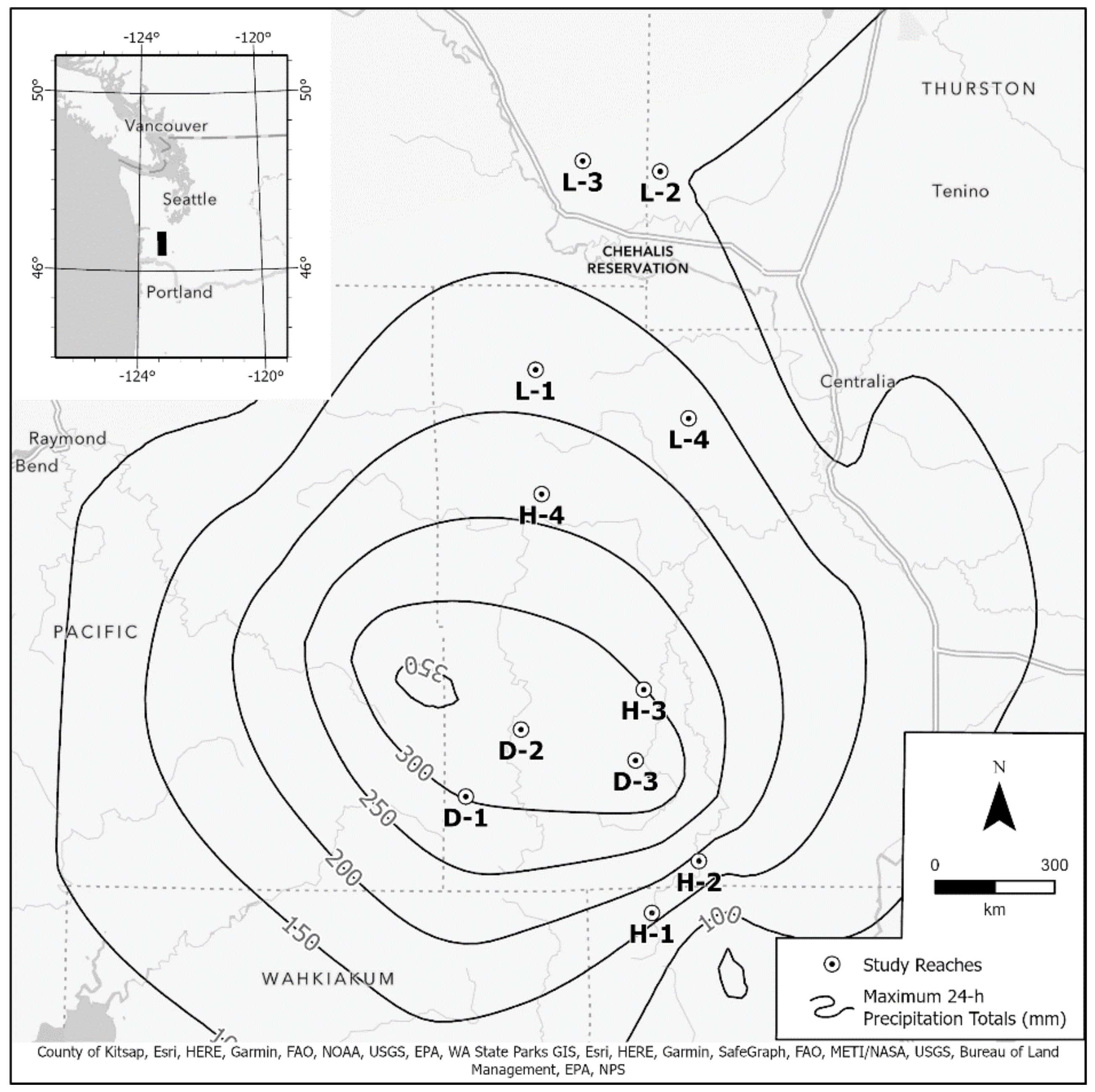
2.1. Study Reaches

The study area was impacted by a severe storm in 1–4 December 2007 (Figure 1). Peak storm flows of 1724 m³/s at Chehalis River in Doty WA (USGS Hydrologic Unit—17100103) were 2.1 × larger than the next highest flow recorded over the 79-year record at this gauge. The storm produced 20–40 cm of rain over three days. The disturbance agent, heavy rain, was not distributed evenly across the landscape and higher elevation reaches received the most precipitation, which fell on top of a light snowpack. Precipitation totals from the December 1st through 4th storm varied greatly among the sample reach estimates based on three gauges and GIS interpolation of 24 h. maximums (70–90% of total) (Figure 1). All watersheds above the study reaches received more than 100 mm of precipitation during the storm and flooded over bank for more than a day.

Our eleven study reaches were all small- to moderate-sized streams with watershed area upstream of study reaches ranging from 5.3 to 45.1 km² (mean 13.2 km²) (

Table 1. Reach characteristics on eleven reaches: immutable watershed characteristics calculated with GIS with baseflow and reach slope field measured at low flood (L), high flood (H), and debris flow (D) disturbance categories.

	L1	L2	L3	L4	H1	H2	H3	H4	D1	D2	D3
Mean Basin Slope (%)	25	19	16	20	31	34	25	30	50	39	47
Basin % Canopy	80	78	77	80	53	50	73	72	92	74	90
Watershed Area (km2)	7.1	9.1	7.9	12.9	45.1	14.3	28.5	11.2	5.3	18	9.7
Mean Basin Elevation(m)	372	293	254	165	387	393	326	390	552	567	524
Maximum Elevation (m)	686	421	418	272	811	756	945	737	799	988	925
Baseflow (m3/s)	0.02	0.02	0.05	0.01	0.13	0.04	0.05	0.04	0.01	0.11	0.02
Reach Slope (%)	4.08	2.7	6.1	0.49	0.57	2	0.19	1.1	4.05	3.4	1.82

). Channel gradient of the study reaches ranged from 0.5 to 3.1% (mean 1.74%), and baseflow ranged from 0.01 to 0.13 m³/s (mean 0.05 m³/s) (Table 1).

Our study reaches represented a gradient of rainfall intensity (Figure 1). We assigned our study reaches to one of three disturbance-intensity categories: debris flow (D), high flood (H), and low flood (L). Assignment of reaches to the two flood intensity categories (high flood, low flood) was based on relative proximity of each reach to the area of greatest rainfall. The three reaches in the debris flow disturbance category were all located in the area that received the most precipitation, storm rainfall totals over 350 mm. High flood reaches experienced precipitation totals ranging from 250 mm to 350 mm and the low flood reaches received from 150 mm to 250 mm (Figure 1).

2.2. Reach Description

The study examined the physical habitat and invertebrate communities at 11 stream reaches located in the headwaters of the Chehalis River in western Washington State. These reaches were selected due to the availability of data collected in 1997 by the Washington State Department of Ecology and U.S. Environmental Protection Agency (DOE/EPA) during a systematic biological survey of streams in western Washington [38,39]. We identified the locations of those reaches again in 2008 using GIS coordinates.

Average annual precipitation in the study area is approximately 1500 mm. However, precipitation varies greatly with elevation, with higher elevations receiving more annual rainfall. Maximum elevations in the watersheds drained by the sampled stream reach range from 270 m to nearly 1000 m. Average monthly water temperatures are roughly 17 °C in summer and 3 °C in winter.

The stream reaches were all located in watersheds that are managed primarily for commercial wood production. The most common conifer tree species in the study areas are Douglas-fir (Pseudotsuga menziesii), western red cedar (Thuja plicata), and western hemlock (Tsuga heterophylla). Red alder (Alnus rubra) is a common deciduous tree species, especially in riparian areas. An extensive road network to facilitate forest management serves the region, with larger mainlines and a network of secondary roads throughout the landscape. The primary forest in the study area was logged in the early and mid-20th century. Therefore, the overstory vegetation throughout nearly all the watersheds tributary to our study reaches was less than 100 years old.

2.3. Physical Habitat Characterization

Reach-level physical habitat data were collected annually in late summer from 2008–2012 and 2016. We focused on physical variables—canopy closure, channel dimensions, and instream features—that could characterize the sample reach and capture the channel attributes most likely to be altered by hydrologic disturbance.

Our study reaches were each 100 m in length. Study reaches were subdivided into 10 m segments. Stream gradient was measured using a laser rangefinder (TruPulse 200; St. Louis, MO, USA). Substrate size was characterized by estimating areal coverage of seven particle size categories (fines <1 mm, sand 1–4 mm, fine gravel 4–16 mm, coarse gravel 16–64 mm, cobble/rubble 64–256 mm, and boulder > 256 mm, as well as percentage of bedrock substrate) in each 10m segment and averaged for the reach. Pieces of wood were counted within the bankfull width and assigned to one of three size categories based on diameter (small 0.1–0.3 m, medium 0.3–0.8 m, and large > 0.8 m). A piece of wood was classified as functioning if it was within the wetted channel at summer low-flow, total wood was all functioning pieces. Mean bankfull channel widths and wetted widths were measured at each 10 m segment boundary. Percent of the wetted channel occupied by riffle, run/glide, and pool features was estimated in each segment and averaged for the reach. Hemispherical photographs taken from 1 m above the stream channel surface each year at 10, 30, 50, 70, 90 m distances along the reach were used to track the recovery of channel shade. Stream temperatures were measured hourly with a submerged thermistor (Onset HOBO Water Temperature Pro v2 Data Logger; Bourne, MA, USA) at each study reach. Water temperatures post-storm were compared using two metrics: 7-day mean daily maxima temperatures and 7-day mean daily minima during summer (6/21st–9/21st). Instruments were checked for accuracy prior to deployment. During invertebrate sampling Wolman pebble counts across each sampled riffle were completed by randomly selecting >100 substrate particles and sorting the lengths of the median axes into bins (bins: 0–1, 1–2, 2–4, 4–8, 8–16, 16–32, 32–64, 64–256, >256 mm). Substrate conditions for each sampled riffle were characterized by calculating the % <2 mm and the diameter of the 50% particle size (D50).

In addition to physical habitat surveys, we characterized topographic features adjacent to the study reach and in the upstream watershed using standard GIS tools and LiDAR-derived topographic data. The topographic metrics were: Mean Basin Slope, Basin % Canopy Cover, Watershed Area, Mean Basin Elevation, Maximum Elevation, and Channel Slope (%). A long-term record of Chehalis River discharge collected near Doty WA (USGS Hydrologic Unit—17100103), was used for historical comparisons and annual trend information. We also measured summer discharge annually during the macroinvertebrate sampling in late July at each study reach by measuring width, depth, and water velocity (at 0.6 depth) at a minimum of 20 equally spaced cells. Cells were summed to estimate summer discharge.

2.4. Macroinvertebrate Sampling

Benthic macroinvertebrates were collected during second half of July annually from three riffles, usually in the downstream half of the study reach. Three Surber samples (0.09 m², 250 µm mesh) were collected and composited into one sample for each sampled riffle (0.27 m² total sample area per riffle; total sample area per study reach—0.81 m²). Substrates to a depth of 20 cm were removed and brushed into the collection net of the sampler. Samples were fixed in the field with 95% ethanol for transfer to the laboratory.

Invertebrates collected in the samples were enumerated and identified in the laboratory. Large samples (>1000 individuals) were sub-sampled. To sub-sample, samples were evenly distributed on a gridded tray and squares were randomly selected and sorted until more than 1000 animals were obtained. Samples ranged from 25–100% sorted. Most of the immature aquatic insects were identified to genus or species, including Chironomidae.

After sorting and identification of samples, individual species were weighed by drying at 70 °C, placing the samples in desiccators for a minimum of 24 h, and then weighing using a Mettler Toledo (AG 2040, Greifensee, Switzerland) balance with a resolution of 0.0001 g. Larger organisms were individually weighed. Organisms too small to weigh individually were weighed as a group and an estimated weight was calculated by dividing total weight by number of individuals. For small species where insufficient numbers of individuals were collected for their combined dry weight to exceed the scale detection limit, half the detection limit (0.00005 g) was assigned as the weight.

DOE/EPA Methods—The 1997 DOE/EPA survey was conducted from 7/1 to 9/1 [38]. Physical habitat information was collected using Environmental Monitoring and Assessment Program (EMAP) protocols for a 150 m reach [39,40]. Macroinvertebrates were sampled from five riffles with a D-frame kick net (500 µm mesh). Five riffle samples at each reach were combined and 300 organisms identified to the finest practical taxonomic level [38]. Sample methods we used for characterizing reach-level physical habitat were similar as those used in the DOE/EPA survey. The DOE/EPA study used a modified convex densiometer [41] and took the mean of multiple measures along the sample reach to estimate average shade. We used hemispherical photographs taken at mid-channel at five locations. Large wood measurements differed slightly as we measure wood in active channel versus within bankfull, which likely led to higher estimates in DOE/EPA study. The DOE/EPA method for sampling invertebrates also differed as we identified some invertebrates to finer taxonomic categories and used a finer sampling mesh. The DOE/EPA effort identified 300 organisms per sample versus a minimum of 1000 in the post-disturbance sampling.

Comparisons of our post-storm results with the results from the 1997 DOE/EPA survey need to be interpreted carefully. The 2007 storm occurred ten years after the DOE/EPA samples were collected; we have no information on assemblage structure or habitat immediately prior to the December 2007 storm. The DOE/EPA sampling methodologies also differed slightly from those used post-storms. In addition, due to the range of collection dates we tried to avoid discharge related metrics (e.g., wet width, mean depth) in between study comparisons. Nonetheless, we believe the DOE/EPA data do provide temporal context for evaluating the post-storm responses and subsequent recovery of physical and biological system properties.

2.5. Data Analysis

We compared pre-storm conditions, as represented in the DOE/EPA data, to conditions in summer following the December storm to characterize the short-term impacts on % shade, bankfull width, and total wood. In the post-storm data collected from 2008–2016, we examined the changes in those features over time, as well as wet width, % fine sediment, and stream temperature (maximum and minimum).

Comparison of macroinvertebrate community characteristics pre-storm versus immediately post-storm was based on EPT (Ephemeroptera, Plecoptera, and Trichoptera) and Chironomidae metrics. With more detailed invertebrate data sets collected from 2008 through 2016 we used additional community metrics to investigate instream community changes over time. The 2008–2016 evaluations included species richness, overall abundance, percentage of multi-voltine species, and percent of scraper feeding type [42] for functional feeding and habit designations). Species richness, in addition to at reach/year comparisons, total richness at reaches through time and total category richness were calculated and presented as percent of total richness. Sampled species abundance and calculated biomass measurements were converted to number and mg per m², respectively. Individual species abundance was classified as percentage of total: abundant (>1%), common (<1% and >0.01%), and rare (<0.01%). One taxon, a snail from Juga spp. (Semisulcospiridae), because of its large relative size and limited distribution, was individually analyzed.

Abundance of species (individuals/m²) with known sensitivity to fine sediment was examined to assess post-storm fine sediment regime [43]. Eleven fine sediment sensitive species used in this analysis: Heterlimnius sp. (Elmidae); three mayflies (Drunella doddsii (Ephemerellidae), Epeorus sp., and Rithrogena sp. (Heptageniidae)), and three stoneflies (Despaxia augusta (Leuctridae); Hesperoperla pacifica (Perlidae), and Megarcys sp. (Perlodidae)) and four caddisflies (Neophylax rickeri (Thremmatidae), Rhyacophila angelita gr., and Rhyacophila hyalinata gr. (Rhyacophilidae), and Arctopsyche grandis (Hydropsychidae)).

We used generalized linear mixed models (GLMM) to evaluate the response of biotic and abiotic characteristics of the disturbed reaches to storm intensity. With the GLMM’s we assume that the response variable follows an exponential family ith mean μ, dispersion parameter $\varphi$, and link function $g\left(.\right)$ [44]. We further assume that μ is linearly associated with model covariates after link transformation, specifically:

$$g\left({\mu }_{ijk}\right)={\beta }_0+b_{0i}+{\beta }_{1}Tr{t}_i+{\beta }_{2}Yea{r}_j+{\beta }_{3}Tr{t}_i\times Yea{r}_j$$

Here, $Tr{t}_i$ denotes the flood category of location i with three levels (D, H, and L), $Yea{r}_j$ denotes the measurement year j (with two levels when comparing the pre-storm and post-storm characteristics and six levels for the repeated measure of the response after the storm). $Tr{t}_i\times Yea{r}_j$ is the interaction of flood category i and year j, which allows temporal trends to vary by flood category. A random intercept $b_{0i}$ is included to account for correlation among measurements taken at the same reach. The model form was consistent among all response variables, but the distributions and the link functions differed depending on the nature of the response variable. The distributions and link functions for each response variable are listed in

Table 2. The distributions and link functions of the GLMM models for pre- and post-storm biotic and abiotic response variables and 2008–2016 storm biotic and abiotic response variables.

Response (y)	Distribution	Link Function/Transformation
	Biotic Characteristics—Before and After Storm
% EPT	Quasi-Binomial	Logit
% Midge	Quasi-Binomial	Logit
	Abiotic Characteristics—Before and After Storm
Bankfull Width	Gaussian	Log(y)
% Shade	Quasi-Binomial	Logit
Total Wood	Quasi-Poisson	None
	Biotic Characteristics—After Storm
Abundance	Gaussian	Log(y)
Richness	Quasi-Poisson	Log
% EPT	Quasi-Binomial	Logit
% Midge	Quasi-Binomial	Logit
% Multi-voltine	Quasi-Binomial	Logit
% Scraper	Quasi-Binomial	Logit
Sediment Intolerant Species	Gaussian	Log(y)
	Abiotic Characteristics—After Storm
Max Temperature	Gaussian	None
Min Temperature	Gaussian	None
Total Wood	Quasi-Poisson	Square Root
Bankfull Width	Gaussian	1/y
Wet Width	Gaussian	None
% Fine Sediments	Quasi-Binomial	Logit
% Canopy Closure	Quasi-Binomial	Logit

. All models were fit in R [45] using package nlme [46]. Transformed values were back transformed for presentation in figures.

In the pre- and post-storm reach characteristics comparisons, the mean pre-post response difference for each flood category was estimated using three contrasts (L2–L1, H2–H1, and D2–D1). We also estimated differences in relative storm response among the three flood categories ((H2–H1)-(L2–L1), (D2–D1)-(L2–L1), and (D2–D1)-(H2–H1)). Results are displayed in figures; calculated contrast estimates are included as Appendix A Figure A1, Appendix B Figure A2 and Appendix C Figure A3.

The differences in abiotic and biotic characteristics after the storm starting in 2008 to 2016 are compared in three ways. Differences in abiotic and biotic characteristics post-storm were compared between the disturbance categories after the storm in 2008 (D8–H8, D8–L8, and H8–L8), as well as the average annual change of the response variables for each disturbance category in the eight-year post storm period (TrendD, TrendH, and TrendL). Finally, the linear change of the reach characteristics was compared between the disturbance categories (TrendD–TrendH, TrendD–TrendL, and TrendH–TrendL).

Agglomerative hierarchical clustering compared the macroinvertebrate assemblage for each reach for each year of post storm sampling (11 reaches × 6-year combinations). The method clusters similar reaches together based on assemblage similarity [47]. We used the Sorensen distance measure and flexible beta (−0.25) for the clustering of 253 species. Taxonomy established unique species. Where no species-level identifications were possible a higher taxonomic level was used to account for a single taxon (e.g., Muscidae, Capniidae). Clustering groups reaches and/or years with high similarity illustrates the relative difference among reaches. The resulting dendrogram is scaled as a percentage of total information by the amount lost in each step of classification [48].

We augment the first classification with a two-way classification which clusters species that are similarly distributed during the study [49]. In the two-way classification, Y-axis is a classification of reaches by macroinvertebrate assemblages, whereas the X-axis classifies individual species into clusters by similarity in their responses at reaches and time [47,49]. We transformed abundance to presence or absence (not detected) and assumed a single occurrence represented the presence of a population. The P/A analysis both reduces impact of abundant species and expands/highlights presence of rare and very rare species. Reach/year (Y) and individual/groups of species (X) form clusters and isolated occurrences, intersections in the matrix show disturbance influence and emphasizes species habitat relations, including rarity.

Biological diversity was heavily influenced by the presence of rare species (those comprising <0.01% of total abundance). We examined rare species distribution through the years following the disturbance with three approaches. We compare rare species overall contributions to abundance and biomass, and % rare species richness among disturbance categories. Secondly, we examine rare species occurrences in the two-way classification of individual species in P/A analysis where isolated species, separated both by X-axis and Y-axis classifications across disturbance intensities and through time, are identified. Thirdly we measure annual turnover rate from 2008 to 2012 by calculating the proportion of species that were not present from the previous year or new presences. We calculate annual turnover by:

t = (species only present at time 1 + species only present in time 2) / (total species time 1 + total species time 2) [50].

3. Results

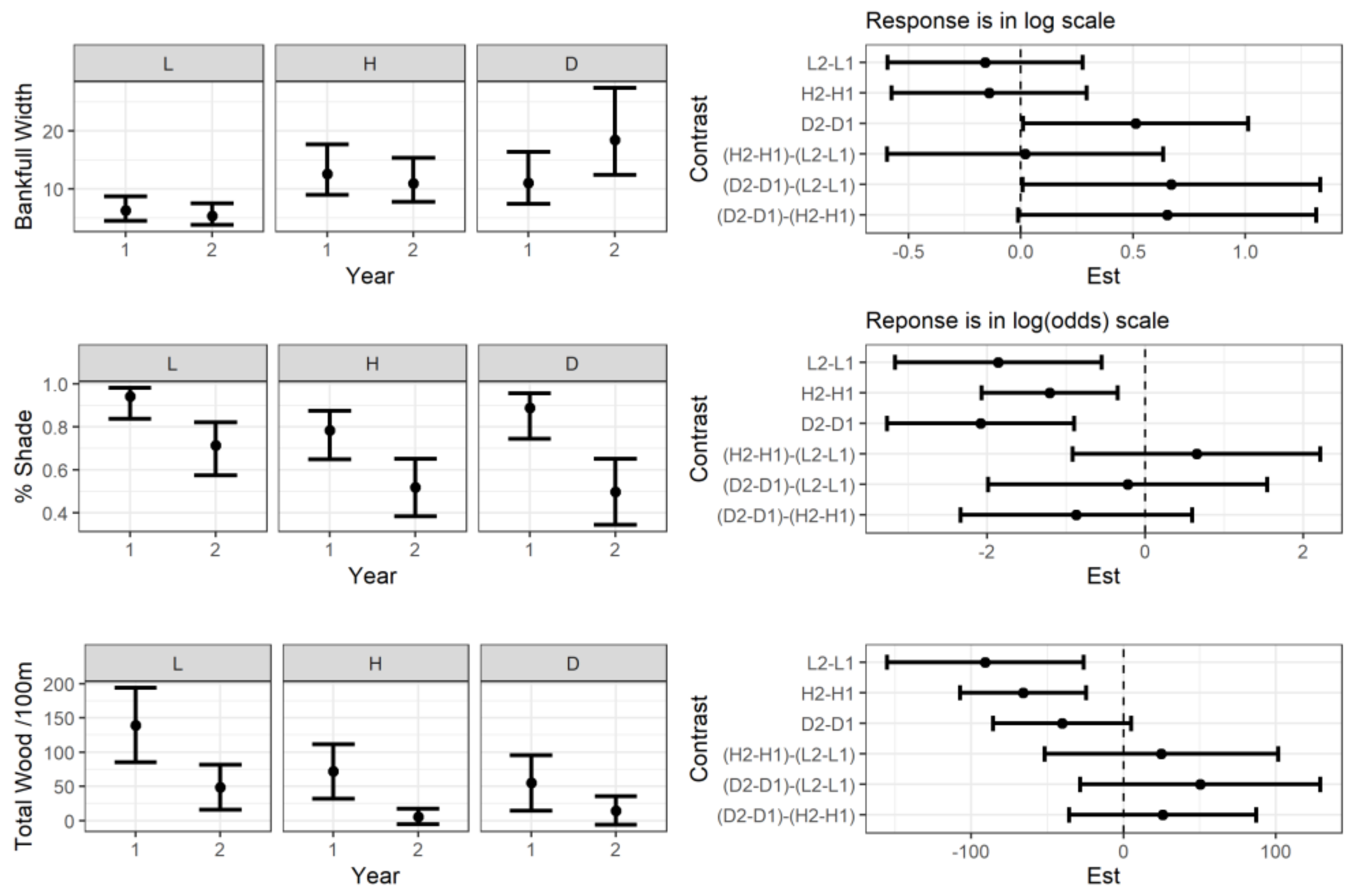
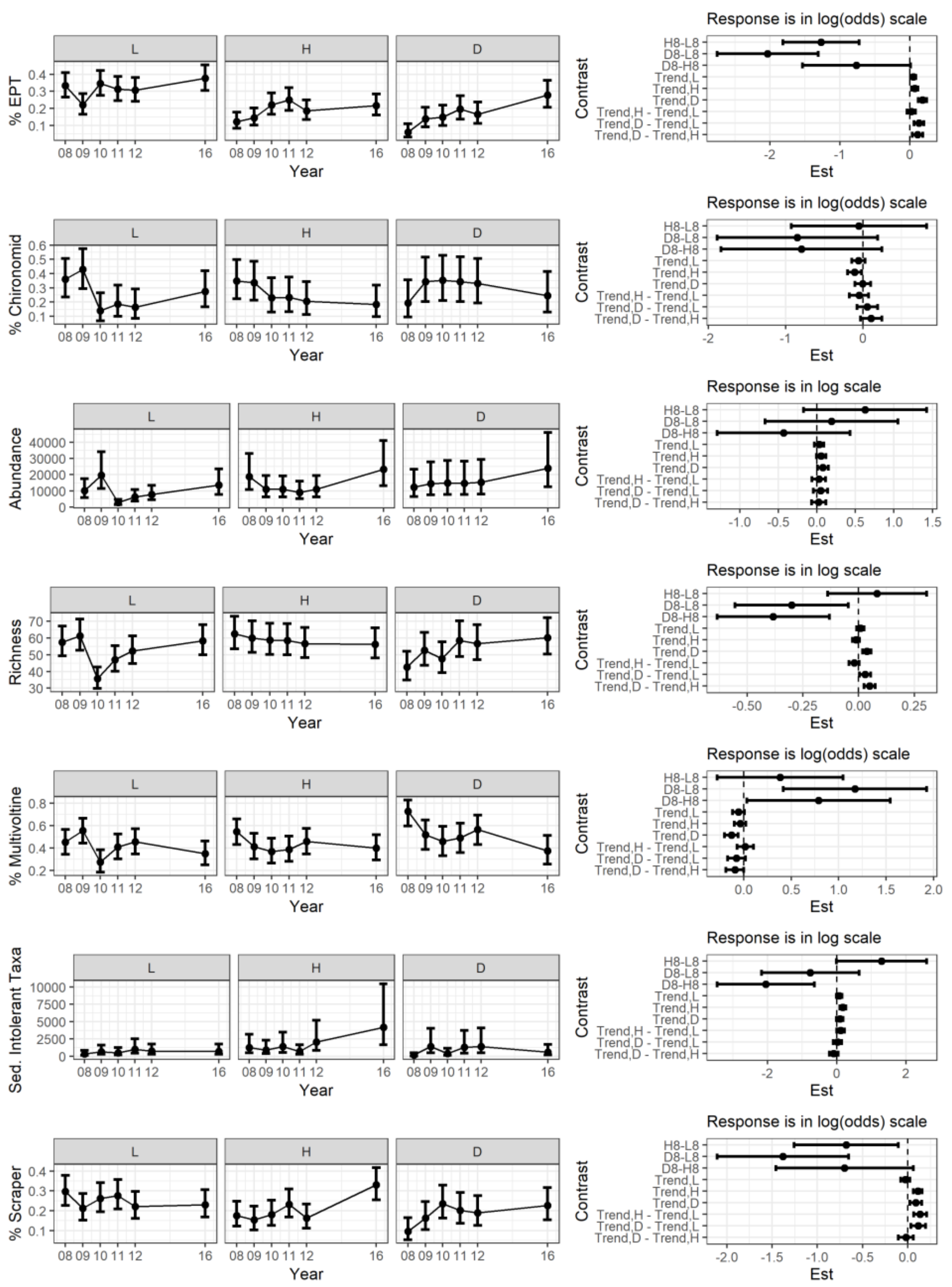
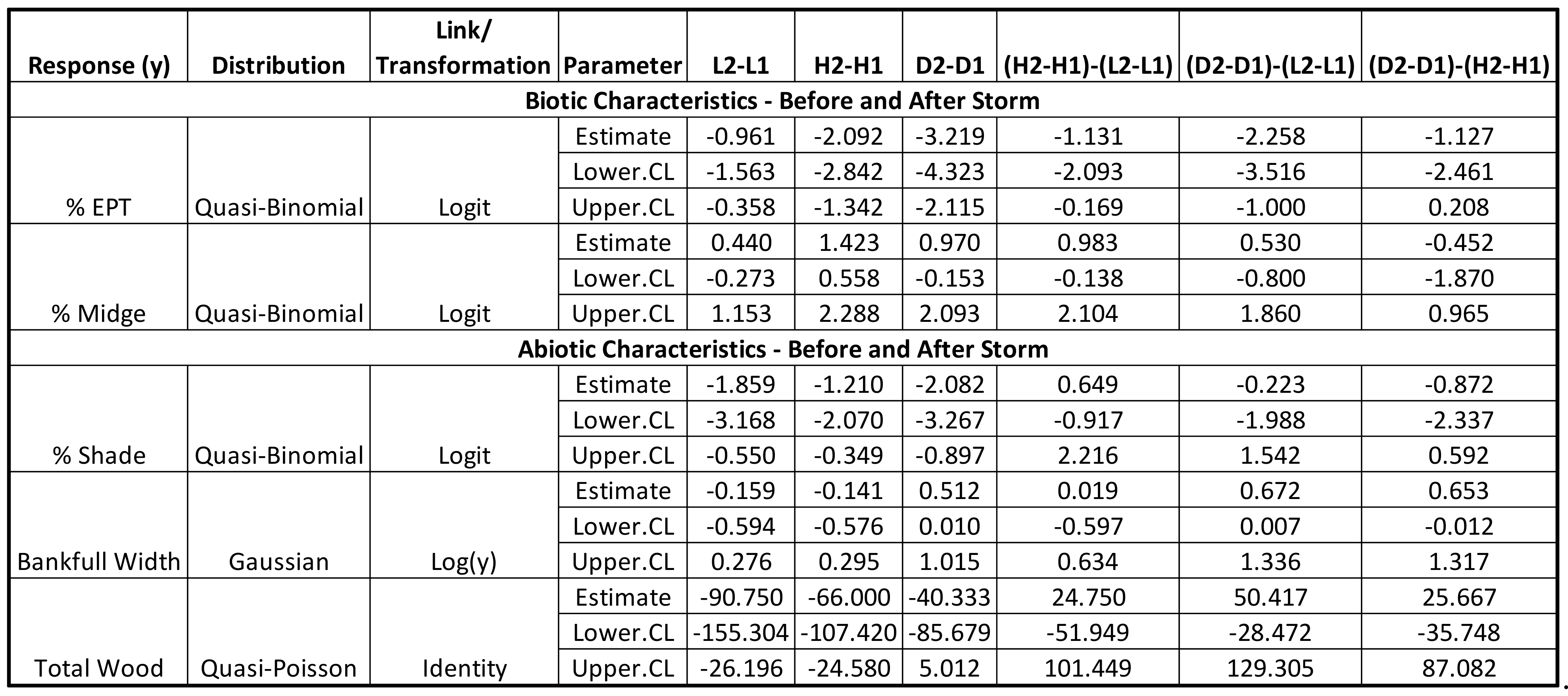
3.1. Abiotic and Biotic Changes before and after Storm

Figure 2 and Figure 3 present GLMM results with the left panel showing back transformed modeled estimates of mean with 90% C.I. for each disturbance category and the right panel has two sets of contrasts. The first is between years (1997 vs. 2008) and the second is the difference in change between categories.

Bankfull Width—Pre-storm and post-storm bankfull widths were not different in L and H reaches. Mean bankfull widths increased post storm at D reaches (Figure 2). Bankfull width is estimated to be 7 to 16 m before the storm and 12 to 27 m after the storm for D reaches. All three D reach contrasts show some evidence of increased bankfull widths after the storm (Figure 2—contrasts 3,5,6).

Shade—We found evidence for less shade for all three flood categories after the storm (Figure 2, contrasts 1–3). Estimates of shade for L reaches indicated a likely to be 80 and 98% pre-storm and 55 to 84% post-storm with lower ranges for other categories. The extent of change between reach categories was similar with all declining (Figure 2, contrasts 4–6).

Total Wood—Total wood was lower post-storm versus pre-storm for all three flood categories (Figure 2, contrasts 1–3). The pieces of wood per 100 m are likely to be 85 to 194 pre-storm and 15 to 82 post-storm and for L reaches, 32 to 112 and 0 to 17 for H reaches, and 15 to 95 and 0 to 36 for D reaches (Figure 2). It is unclear how the storm effect may have differed among the three categories—i.e., the uncertainty in the values was greater than the differences (Figure 2). The relative change before and after the storm of total wood reduction was similar across categories (Figure 2, contrasts 4–6).

Percent EPT—The estimated % EPT of total abundance decreased after the storm in all the disturbed reaches with the least decrease for L reaches and the most in D reaches (Figure 3). We estimated % EPT of 45 to 67% pre-storm and 23 to 45% post-storm for L reaches, 42 to 65% and 7 to 21% for H reaches, and 50 to 74% and 2 to 15% in D reaches. Our results suggest that the effect of storm on EPT abundance was greater on H and D reaches compared to L reaches (Figure 3, contrasts 4, 5).

Percent Chironomidae—Estimated % Chironomid was higher at H reaches after the disturbance with some evidence for increases at L and D reaches (Figure 3, contrasts 1–3). Percent Chironomid was likely 13 to 36% pre-storm and 20 to 46% post-storm for L, 5 to 20% pre-storm and 20 to 45% post-storm in H, and 3 to 20% pre-storm and 10 to 35% post-storm for D reaches. Estimates of differences in storm impact among the three disturbance categories were not clear (Figure 3, contrasts 4–6).

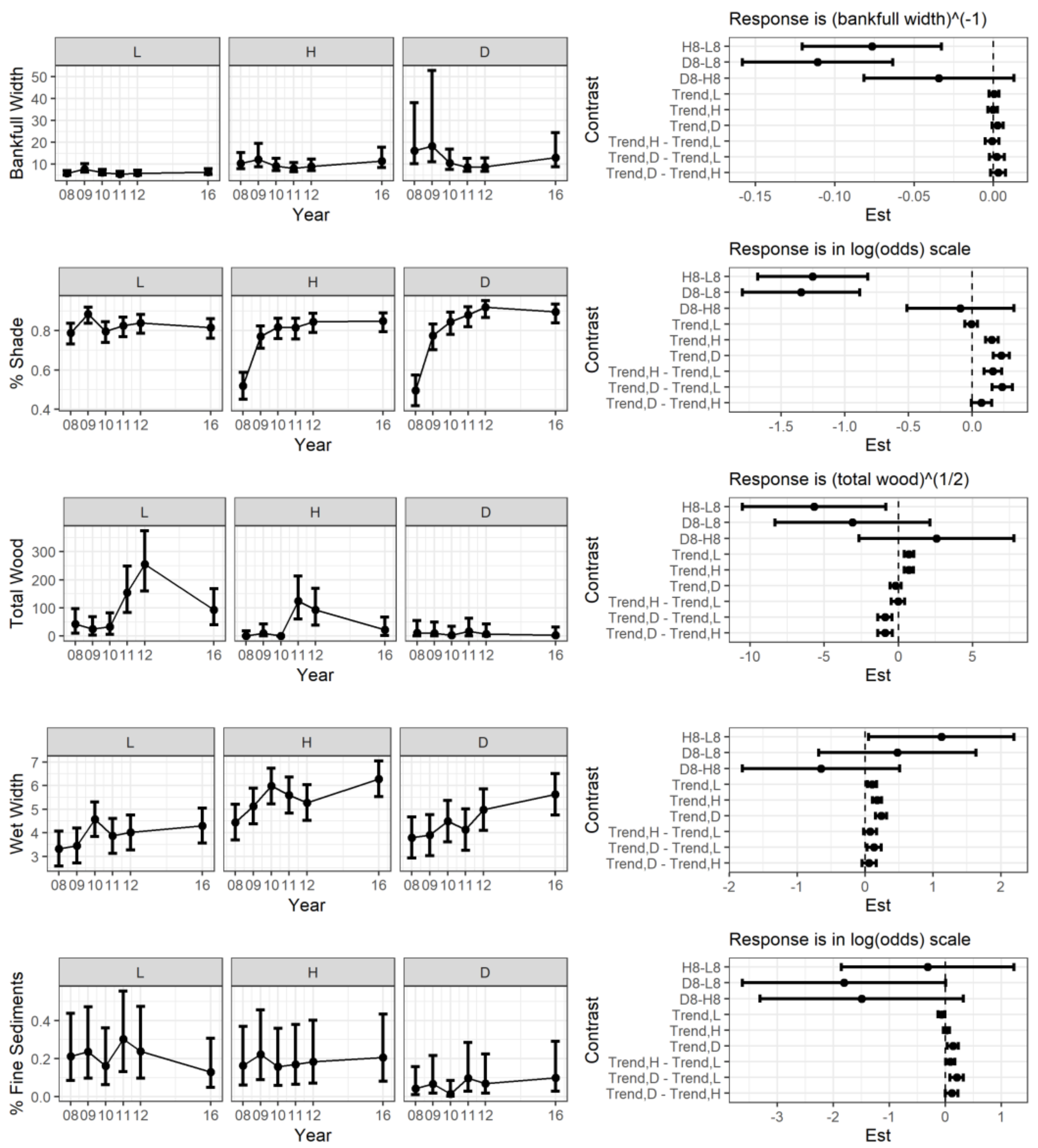
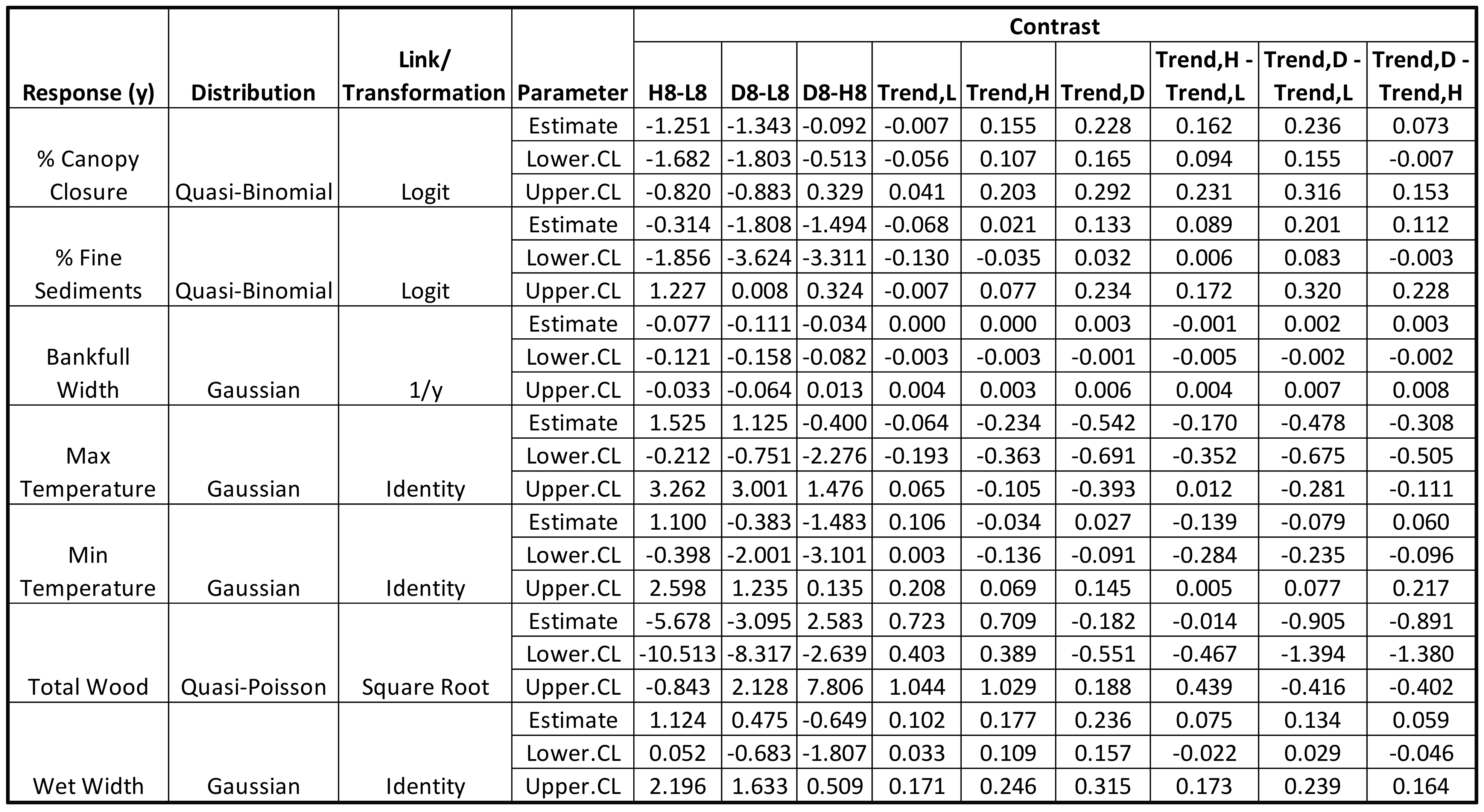
3.2. Stream Temperature and Physical Features Changes after the Storm

Figure 4, Figure 5 and Figure 6 present GLMM results with the left panel showing back transformed modeled estimates of mean with 90% C.I. for each disturbance category through time. The right panel has nine contrasts in three sets. The first three contrasts are between each category in 2008, the next three contrasts show the trend for each category, and the final three contrasts show the difference in trend between categories.

Stream Temperature—Comparison of post-storm maximum temperature among the three disturbance categories showed estimated differences with wide ranges of uncertainty. The difference in expected maximum temperature for H treatments was approximately 1.5 °C higher than L treatments. The estimated ranges overlap (Figure 4). The maximum temperature was estimated to be 18 to 21 °C at L, 20 to 22 °C at H, and 19 to 22 °C at D reaches in 2008. We estimated a mean decrease in temperature trend as H and D reaches, most strongly at D reaches (Figure 4, contrasts 5,6,8,9). An elevated maximum temperature was observed at both L and H reaches for three years (2010–2012) but was not observed at D reaches (Figure 4).

Estimates of minimum temperature were 13 to 15 °C in L, 14 to 16 °C for H, and 13 to 15 °C for D reaches. There was also an increase in minimum temperature observed at both L and H reaches for three years (2010–2012) (Figure 4). No changes in minimum temperatures were observed at D reaches (Figure 4, contrast 6).

Bankfull Width—A bankfull width range of 5 to 7 m for L, 8 to 15 m for H, and 10 to 40 m for D reaches were found after the storm. At two of the D reaches multiple channels were formed following the storm, spreading to valley edges but returned to a single channel by year three (Figure 5).

Percent Shade—Post-storm % shade was lower at H and D than L reaches (Figure 5, contrasts 1–3). The post-storm percent shade was estimated to be 73 to 84% for L, 45 to 59% for H, and 42 to 57% for D reaches. There was an increase in percent shade D and H reaches, with most of this increase occurring during the first two years after the storm (Figure 5, contrasts 5,6). There was minimal change in shade for L reaches across the post-storm period (Figure 5, contrast 4). In 2016, the % shade was estimated to be 76 to 86% in L, 80 to 89% in H, and 84 to 94% in D reaches (Figure 5).

Total Wood—There was more total wood (pieces/100 m) after the storm at L than H reaches (Figure 5, contrast 1), with no clear evidence of differences between D and H reaches (Figure 5, contrasts 2,3). Total wood was estimated to be 10 to 97 for L, 0 to 18 for H, and around 0 to 54 pieces per 100 m for D in 2008. The annual mean trends post storm in total wood for H and L reaches were positive overall, partially driven by high wood abundance in 2011 and 2012 (Figure 5, contrasts 4,5). The total wood is estimated to be 39 to 168 for L and 2 to 67 pieces per 100 m in H reaches and 0 to 35 in D reaches in 2016 (Figure 5).

Wet Width—Wet width after the storm had a positive trend in all categories (Figure 5, contrasts 4–6). Mean estimates for D reach wet widths were intermediate to the L and H widths (Figure 5).

Percent Fine Sediment—Percentage fine sediments showed evidence of being lower for D reaches than H or L reaches in 2008 (Figure 5, contrasts 2,3). The estimated post-storm % fine sediment ranged from 8 to 44% for L, 6 to 37% for H, and 1 to 16% at D reaches. Estimated trends showed some evidence of an increase over time at D and a decrease at L reaches, (Figure 5, contrasts 4,6). Trends for H reaches were inconclusive (Figure 5, contrast 5).

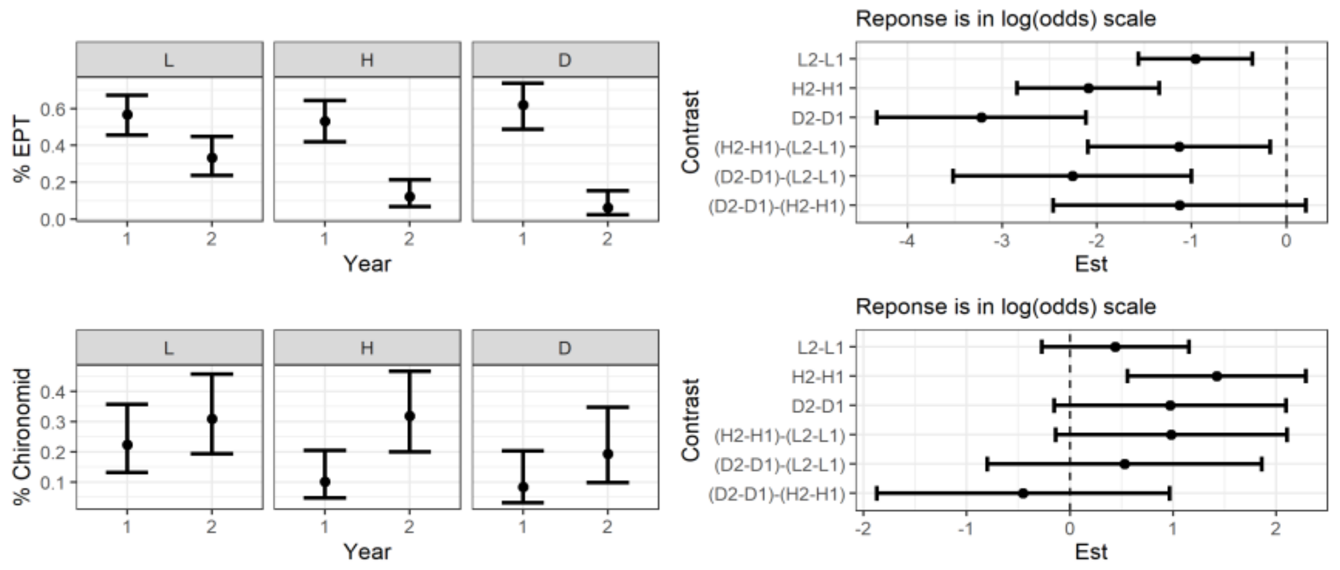
3.3. Macroinvertebrates Changes after the Storm

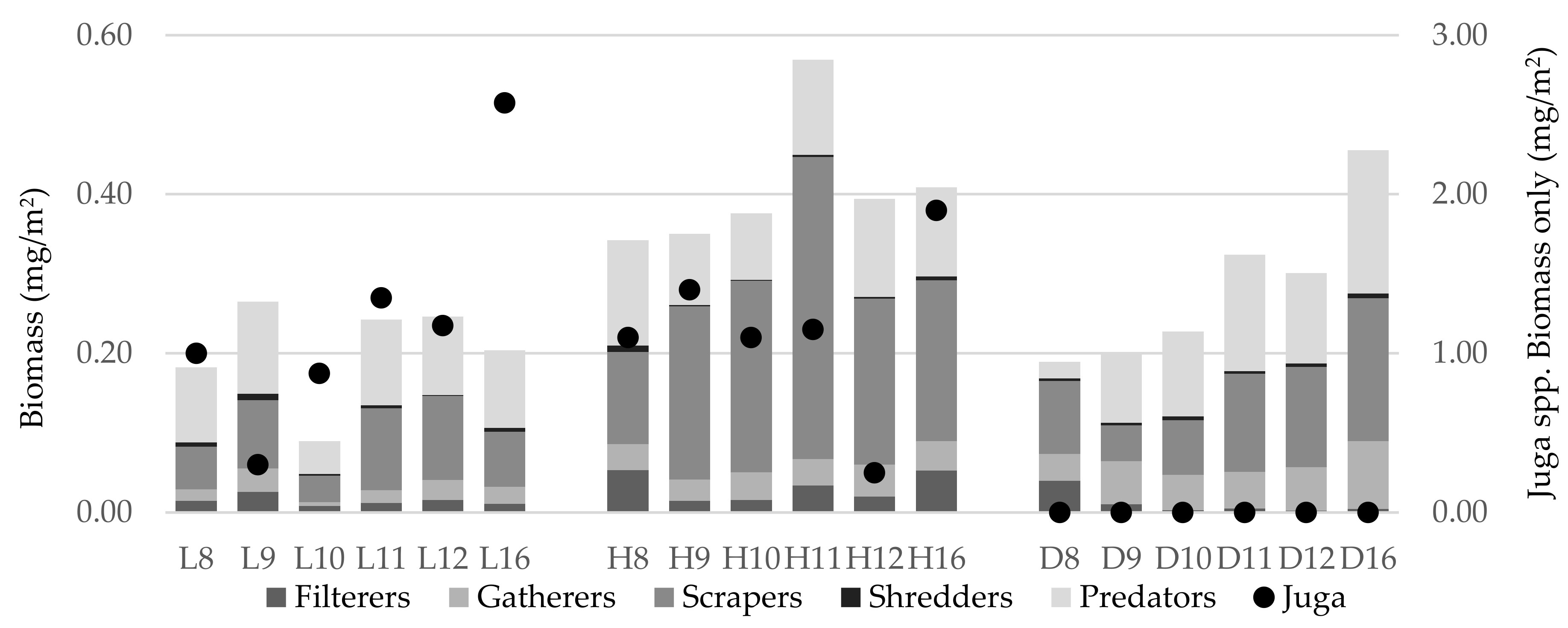
Percent EPT—There was a higher post-storm % EPT in L compared to H and D reaches and some evidence that H reaches were higher than D reaches (Figure 6, contrasts 1–3). The estimates of % EPT were 27 to 41% in L, 8 to 18% in H, and 3 to 11% in D reaches in 2008. There was evidence of a post-storm increase in % EPT for all the disturbance categories, most strongly at D reaches (Figure 6, contrasts 4,5,6,8,9).

Percent Chironomidae—The small sample sizes and high variability limited our power to estimate differences among the three disturbance categories in % Chironomid the first year after the storm. The post-storm % Chironomid was estimated to be between 2 to 51% for L, 22 to 50% for H, and 10 to 36% for D reaches (Figure 6). There was evidence of a mean annual decrease in % Chironomid in H reaches and no clear indication of directional changes in % Chironomid for L or D reaches (Figure 6, contrasts 4–6). L reaches were highly variable, including a significant decline after 2009 which is also reflected in other metrics—Abundance, Richness, and % Multi-voltine (Figure 6).

Abundance—The macroinvertebrate density was estimated to be 5818 to 17,507 (individuals/m²) for L, 10,709 to 33,159 (individuals/m²) for H, and 6351 to 23,424 (individuals/m²) for D reaches in 2008. We found no clear evidence of differences in mean abundance among the three disturbance categories in 2008 (Figure 6). There is evidence of an annual increase in abundance in D reaches, less evidence for an increase at H reaches, and at L reaches the direction of trend was not clear (Figure 6, contrasts 4–6).

Two species, the Baetidae mayfly Baetis tricaudatus and a chironomid Micropsectra sp., were the most abundant and each comprised more than 10% of the total abundance. An additional 18 species contributed more than 1% of total abundance and another 50 species comprised between 1% and 0.01% of total. The remaining 183 species contributed less than 0.01% of the total abundance and included 35 species (12.4% of total) that were collected only once or twice. The high chironomid richness (66 species) included mostly species that were rare, as only six (Micropsectra sp., (14.9%), Brillia sp. (4.0%), Tvetenia bavarica gr. (3.6%), Polypedilum sp. (2.1%), Orthocladius complex (1.6%), and Cricotopus sp. (1.0%)) comprising more than 1% of total abundance.

Richness—There was lower post-storm richness in D reaches compared to L and H reaches (Figure 6, contrasts 2,3). Post-storm richness estimates in D reaches were 49 to 67 species for L, 54 to 73 species for H, and 35 to 52 species for D reaches (Figure 6). Most of the 253 species collected during the investigation were rare. Richness was lowest at D reaches and steadily increased over time (Figure 6, contrast 6). Richness remained unchanged in the other disturbance categories, yet compositionally dynamic (Figure 6).

Richness at each reach (all years combined) was 122–150 species. Combining all the species within a disturbance category richness was 198, 204, and 190 species at L, H, and D or 78, 81, and 75% of total study richness (253), respectively.

Percent Multi-voltine—We estimated higher post-storm % multi-voltine in D reaches compared to L and H reaches, with similar values for L and H. The % multi-voltine estimates ranged from 34 to 57% in L, 43 to 66% in H, and 60 to 83% in D reaches in 2008. There was evidence of decrease at D reaches (Figure 6, contrast 6) and no clear evidence at L and H (Figure 6, contrasts 4,5).

Percent Scraper—There was some evidence of higher % scrapers in L reaches compared to D and H reaches in 2008 (Figure 6, contrasts 1,2). Percent Scraper was likely to be 23 to 28% in L, 12 to 25% in H, and 5 to 17% in D reaches. There was evidence of increases in % scraper in D and H reaches through time (Figure 6, contrasts 5, 6), but no clear indication of change for L reaches (Figure 6, contrast 4).

Sediment Intolerance Species Density—There was evidence D reaches supported fewer sediment intolerant species than H reaches in 2008 (Figure 6, contrast 3). Post-storm sediment intolerant species abundance all years was estimated to be from 142 to 857, 506 to 3191, and 56 to 571 (individuals/m²) at L, H, D reaches respectively (Figure 6). All reaches showed evidence of a positive trend, with stronger evidence at H reaches (Figure 6, contrast 5). Abundance, except for the first post year across D reaches, was maintained through time. Including a strong contribution at one H reach in 2016 from the Ephemeropteran, Rithrogena sp. (Figure 6, also, note response in % Scraper).

3.4. Biomass

Biomass analysis was confounded by the presence of the snail Juga spp. due to its large size and absence from the D reaches, including the 1997 collections. Overall, the L and H reaches have approximately twice the overall biomass of D reaches. With Juga spp. removed the assemblage biomasses were similar (Figure 7). Biomass increased at the D reaches after the storm (Figure 7). In addition to Juga spp. there was a strong representation of the scraping functional feeding group at H reaches; more than twice the other disturbance categories, except at the 2016 D reaches (Figure 7).

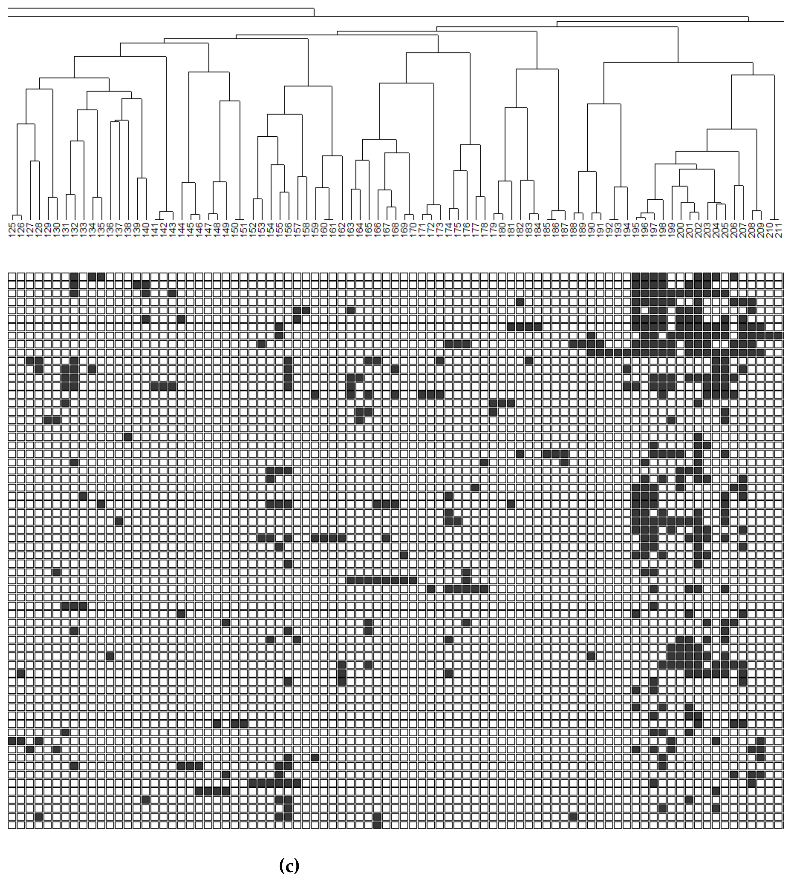
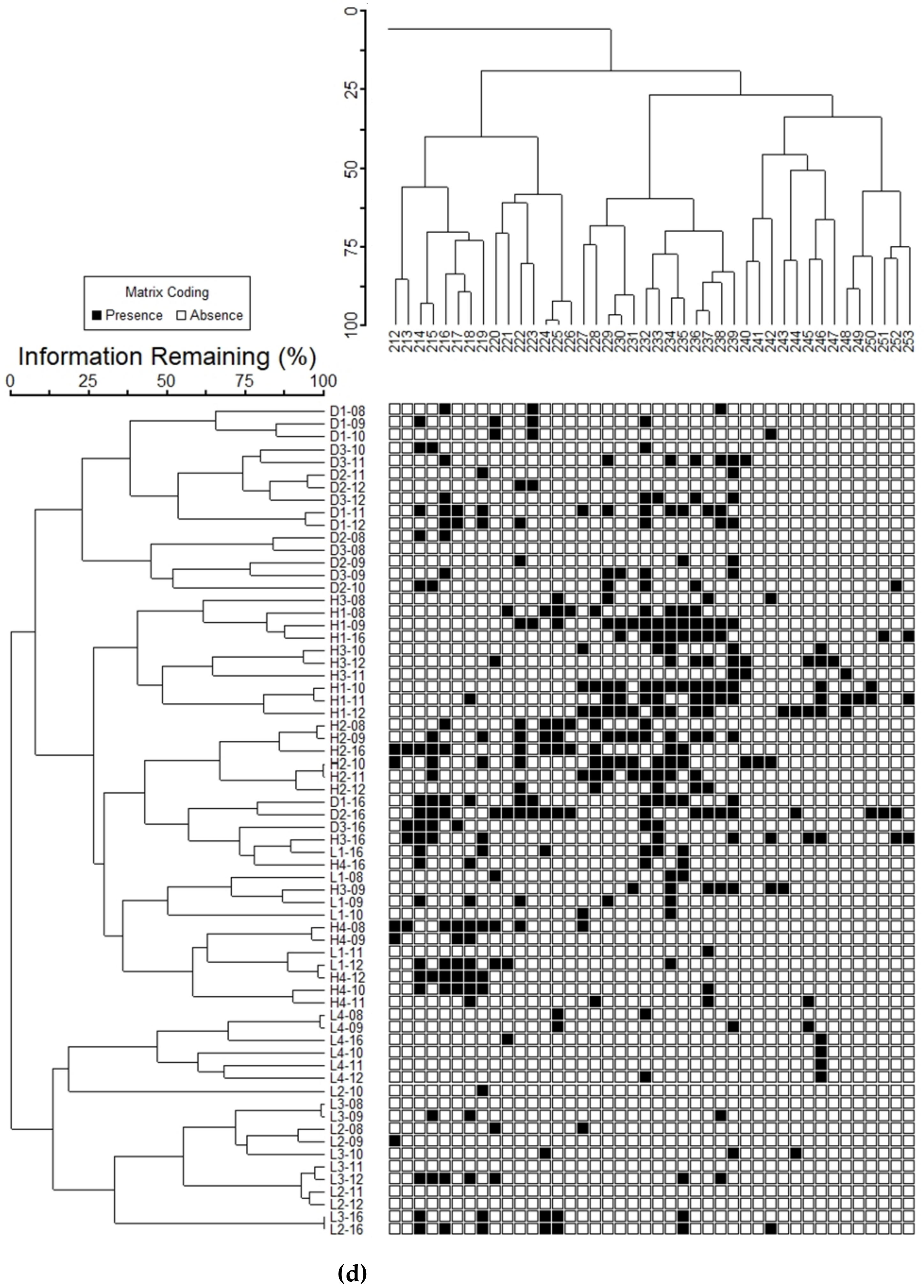
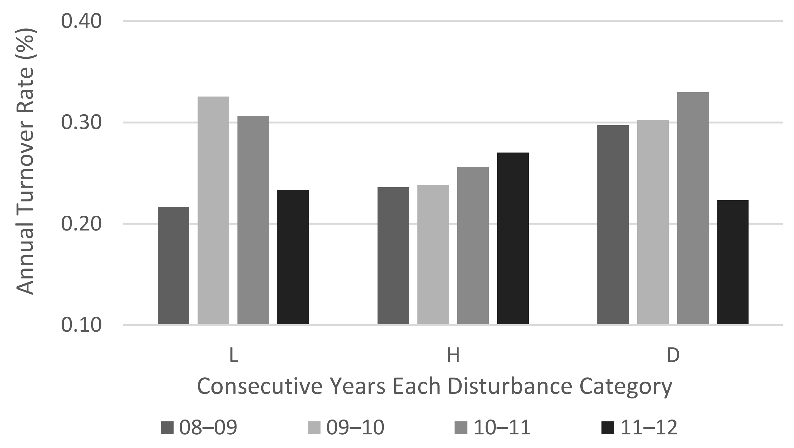
3.5. Community Organization

The first classification on the Y-axis’ clusters each reach and year macroinvertebrate assemblage by similarity (Figure 8a–d). The second classification clusters individual species by similarity of response (P/A distribution) on the X-axis (Figure 8a–d,

Table 3. List of all taxa collected classified in Cluster 1 and Cluster 2. Relative abundances (RA) are A—abundant > 1% of all collections, C—common between 0.01 and 1%, and Rare < 0.01%. Major taxonomic groupings are: A—Acari, E—Ephemeroptera, P—Plecoptera, T—Trichoptera, Co—Coleoptera, D—Diptera (wo/C), C—Chironomidae, G—Gastropoda, M—Megaloptera, and Oth—other organisms). Functional feeding group (FFG) are P—predator, G—grazer, SH—Shredder, S—Scraper, and F—filterer), and fine sediment sensitivity (FSBI) are ES—extremely sensitive, VS—very sensitive, and S—sensitive.

	Cluster 1
	Taxa lowest level	Major group	RA	FFG	FSBI		Taxa lowest level	Major group	RA	FFG	FSBI
	Group 1A					45	Dicosmoecus gilvipes	T	C	S
1	Atractides sp.	A	C	P		46	Synorthocladius sp.	C	C	G
2	Lebertia sp.	A	C	P		47	Antocha sp.	D	C	G	ES
3	Micropsectra sp.	C	A	G		48	Cricotopus sp.	C	A	SH
4	Polypedilum sp.	C	A	SH		49	Eukiefferiella brehmi gr.	C	C	G
5	Sperchon sp.	A	C	P		50	Eukiefferiella pseudomontana gr.	C	C	G
6	Zapada cinctipes	P	A	SH		51	Paraperla sp.	P	R	P
7	Torrenticola sp.	A	C	P		52	Rhyacophila brunnea gr.	T	C	P
8	Oligochaeta	Oth	A	G		53	Hexatoma sp.	D	C	P
9	Dicranota sp.	D	C	P		54	Paraleptophlebia sp.	E	C	G	S
10	Brillia sp.	C	C	SH		55	Lepidostoma sp.	T	R	SH
11	Tvetenia bavarica gr.	C	A	G		56	Krenosmittia sp.	C	C	G
12	Baetis tricaudatus	E	A	G		57	Rheocricotopus sp.	C	C	G
13	Cinygmula sp.	E	A	S	S	58	Yoraperla sp.	P	C	SH	S
14	Calineuria californica	P	A	P	S	59	Clinocera sp.	D	C	P
15	Glossosoma sp.	T	A	S	S	60	Parapsyche almota	T	C	G
16	Simulium sp.	D	A	F		61	Eukiefferiella gracei gr.	D	C	G
17	Sweltsa sp.	P	A	P		62	Rhyacophila hyalinata gr.	T	C	P	ES
18	Nematoda	Oth	C	P		63	Eukiefferiella tirolensis	C	R	G
19	Rhyacophila betteni gr.	T	C	P	S	64	O. (Symp.) lignicola	C	R	G
20	Thienemannimyia gr. sp.	C	C	G		65	Ironodes sp.	E	R	S	S
21	Parametriocnemus sp.	C	C	G			Group 1B
22	Malenka sp.	P	C	SH		66	Dixa sp.	D	C	G
23	Optioservus sp.	Co	C	S		67	Rheotanytarsus sp.	C	C	F
24	Bezzia/Palpomyia sp.	D	C	P		68	Skwala sp.	P	C	P
25	Wormaldia sp.	T	A	F		69	Neoplasta sp.	D	R	S
26	Zaitzevia sp.	Co	C	g		70	Attenella delantala	E	C	G
27	Narpus sp.	Co	C	G		71	Hydropsyche sp.	T	C	F
28	Heterlimnius sp.	Co	A	G	S	72	Heleniella sp.	C	C	G
29	Neophylax rickeri	T	C	S	S	73	Glutops sp.	D	C	P
30	Drunella doddsii	E	C	S	VS	74	Arctopsyche grandis	T	C	F
31	Epeorus sp.	E	A	S	VS	75	Pericoma/Telmatoscopus sp.	D	C	G
32	Hesperoperla pacifica	P	C	P	VS	76	Zavrelimyia sp.	C	R	P
33	Rhyacophila angelita gr.	T	C	P	VS	77	Protzia sp.	A	R	P
34	Eukiefferiella claripennis gr.	C	C	G		78	Paraphaenocladius “n. sp.”	C	C	G
35	Thienemanniella sp.	C	C	G		79	Nilotanypus fimbriatus	C	R	P
36	Diphetor hageni	E	C	G		80	Sperchonopsis sp.	A	R	P
37	Rhithrogena sp.	E	C	S	ES	81	Pacifastacus leniusculus	Oth	R	SH
38	Orthocladius Complex	C	A	G		82	Juga spp.	G	C	S
39	Stempellinella sp.	C	C	G		83	Pisiduim	Oth	C	F
40	Chelifera/Metachela sp.	D	C	U		84	Rhyacophila blarina	T	C	P
41	Serratella tibialis	E	C	G	S	85	Despaxia augusta	P	C	SH
42	Corynoneura sp.	C	R	G	ES	86	Rhyacophila narvae	T	C	P
43	Pagastia sp.	C	C	G		87	Rhyacophila vagrita gr.	T	C	P
44	Acentrella turbida	E	A	G		88	Atylotus/Tabanus sp.	D	R	G
	Cluster 2
	Taxa lowest level	Major group	RA	FFG	FSBI	#	Taxa lowest level	Major group	RA	FFG	FSBI
	Group 2A					171	Allocosmoecus partitus	T	R	P
89	Tanytarsus sp.	C	C	F		172	Psychoglypha sp.	T	R	G
90	Agraylea sp.	T	R	SH		173	Polycelis sp.	Oth	R	P
91	Mideopsis sp.	A	R	P		174	Saetheria tylus	C	R	U
92	Micrasema sp.	T	R	SH		175	Cultus sp.	P	R	P	VS
93	Centroptilum sp.	E	R	G		176	Baetis alius	E	R	G
94	Oreogeton sp.	D	R	P		177	Crenitis sp.	Co	C	P
95	Amiocentrus aspilus	T	R	SH		178	Nixe sp.	E	R	S	S
96	Hydrobiidae	G	C	S		179	Brundiniella sp.	C	R	U
97	Boreochlus sp.	C	R	G		180	Attenella margarita	E	R	G	VS
98	Rickera sorpta	P	R	P		181	Ochthebius sp.	Co	R	P
99	Eukiefferiella brevicalcar gr.	C	R	G		182	Sanfillipodytes sp.	Co	R	P
100	Potthastia gaedii gr.	C	C	G		183	Goera sp.	T	R	S
101	Paratanytarsus sp.	D	R	G		184	Tipula sp.	D	R	SH
102	Potthastia longimana gr.	C	R	G		185	Euryhapsis sp.	C	R	U
103	Oribatei	A	R	P		186	Parorthocladius sp.	C	R	G
104	Sublettea sp.	C	R	F		187	Psilometriocnemus sp.	C	R	G
105	Pteronarcys californica	P	R	SH	S	188	Testudacarus sp.	A	R	P
106	Parakiefferiella sp.	C	R	G		189	Ulomorpha sp.	D	R	U
107	P. umbilicatellus	G	R	G		190	Stygothrombium sp.	A	R	P
108	Bryelmis rivularis	Co	R	G		191	Limnophila sp.	D	R	P
109	Pteronarcella sp.	P	R	SH		192	Frisonia picticeps	P	R	P
110	Stenochironomus sp.	C	R	G		193	Oreodytes sp.	Co	R	P
111	Ephemerella aurivillii	E	R	G		194	Perlinodes aurea	P	C	P	ES
112	Ampumixis dispar	Co	R	F	ES	195	Rhyacophila arnaudi	T	R	P
113	Cryptolabis sp.	D	R	SH		196	Rhyacophila pellisa/valuma	T	R	P
114	Labiobaetis sp.	E	R	S		197	Atherix sp.	D	C	P
115	Meringodixa sp.	D	R	G		198	Turbellaria	Oth	R	P
116	Ptychoptera sp.	D	R	G		199	Baetis flavistriga	E	C	G
117	Hydrobaenus sp.	C	R	S		200	Ecdyonurus sp.	E	R	S
118	Sialis sp.	M	R	P		201	Hesperoconopa sp.	D	R	G	VS
119	Maruina sp.	D	R	S		202	Lopescladius sp.	C	C	G
120	Psychomyia sp.	T	R	CF		203	Demicryptochironomus sp.	C	R	G
121	Cleptelmis addenda	Co	R	B		204	Drunella grandis	E	C	S	S
122	Cinygma sp.	E	R	S		205	Onocosmoecus sp.	T	R	SH
123	Atrichopogon sp.	D	R	B	VS	206	Chrysops sp.	D	R	SH
124	Larsia sp.	C	R	P		207	Pentaneura sp.	C	R	P
	Group 2B–1					208	Hydraena sp.	Co	R	P
125	Eukiefferiella devonica gr.	C	R	G		209	Fluminicola sp.	G	C	S
126	O. (Euortho.) rivicola gr.	C	C	G		210	Brachycentrus occidentalis	T	R	G
127	Oligophlebodes sp.	T	R	S		211	Krenopelopia sp.	C	R	P
128	Ephemerella sp.	E	R	S			Group 2B–2
129	Doroneuria sp.	P	R	P	VS	212	Pedicia sp.	D	R	P
130	Diamesa sp.	C	R	G		213	Psephenus sp.	Co	R	S
131	Agabus sp.	Co	R	P		214	Lara sp.	C	R	SH
132	Timpanoga hecuba	E	R	G		215	Moselia infuscata	P	R	SH
133	Limnesia	A	R	P		216	Cladopelma sp.	C	R	G
134	Microtendipes rydalensis gr.	C	R	F		217	Pseudocloeon sp.	E	R	SH
135	Nilobezzia sp.	D	R	P		218	Natarsia sp.	C	R	P
136	Tokunagaia sp.	C	C	G		219	Pseudosmittia sp.	C	R	G
137	Caudatella sp.	E	R	G	VS	220	Wandesia sp.	A	R	P
138	Gonomyia sp.	D	R	G		221	O. (Euortho.) rivulorum gr.	C	R	G
139	Zapada frigida	P	R	SH	S	222	Dixella sp.	D	R	G
140	Drunella spinifera	E	R	S	S	223	Taeniopterygidae	P	R	SH
141	Suwallia sp.	P	R	P	S	224	Matriella teresa	E	R	SH
142	Megarcys sp.	P	R	P	ES	225	Ablabesmyia sp.	C	R	P
143	Zapada columbiana	P	R	SH		226	Tribelos jucundum	C	R	G
144	Chaetocladius sp.	C	R	G		227	Valvata sp.	G	R	S
145	Parorthocladius sp.	C	R	G		228	Paracladopelma sp.	C	R	G
146	Reomyia sp.	C	R	G		229	Cladotanytarsus sp.	C	R	G
147	Diplocladius sp.	C	C	G		230	Muscidae	D	R	P
148	Parochlus sp.	C	C	G		231	Boreoheptagyia sp.	C	R	G
149	Cardiocladius sp.	C	R	G		232	Baetis notos	E	R	G
150	Isoperla sp.	P	R	P		233	Serratella micheneri	E	R	G
151	Ametor sp.	Co	R	U		234	Parachaetocladius sp.	C	R	G	S
152	Serratella teresa	E	R	G	S	235	Gomphidae	M	R	G
153	Aturus sp.	A	R	P		236	Mesobates sp.	A	R	P
154	Setvena sp.	P	R	P		237	Stilobezzia sp.	D	R	P
155	Neophylax splendens	T	R	S	S	238	Goera archaon	T	R	S
156	Zapada oregonensis gr.	P	R	SH	S	239	Ptychoptera sp.	D	R	u
157	Pteronarcys princeps	P	R	SH	S	240	Metriocnemus sp.	C	R	G
158	Hygrobates sp.	A	R	P		241	Labrundinia sp.	C	R	P
159	Heterotrissocladius marcidus gr.	C	R	G		242	Forcipomyia sp.	D	R	G
160	Constempellina sp.	C	R	G		243	Phaenopsectra sp.	C	R	S
161	Hydatophylax hesperus	T	R	SH		244	Anafroptilum sp.	E	R	G
162	Capniidae	P	C	SH		245	Laccobius sp.	Co	R	SH
163	Rhabdomastix fascigera gr.	D	R	G	S	246	Paratendipes sp.	C	R	G
164	Apatania sp.	T	C	S	S	247	Pseudodiamesa sp.	C	R	G
165	Cryptochia sp.	T	R	SH		248	Agapetus sp.	T	R	S
166	Ameletus sp.	E	C	G		249	Limnophyes sp.	C	R	B	S
167	Drunella coloradensis/flavilinea	E	C	S	S	250	Limonia sp.	D	R	SH
168	Trichoclinocera sp.	D	R	P		251	Nanocladius sp.	C	R	G
169	Rhyacophila vofixa gr.	T	C	P	VS	252	Eukiefferiella coerulescens gr.	C	R	B
170	Kogotus sp.	P	R	P	VS	253	Paraboreochlus sp.	C	R	G

).

Macroinvertebrate assemblages along the Y-axis divide into three broad clusters that generally aligned with our disturbance intensity categories (Figure 8). Reaches/years separate the L cluster in two clusters generally distinct from the H and D group (Figure 8a–d). All D reaches are at the top of the figure (except for 2016 samples) split from L and H reaches (Figure 8a–d). The larger cluster contained three discernible sub-clusters: first the larger contributing area high flood reaches, H3 and H1, separated from the smaller watersheds, H4 and H2 (Figure 8a–d). The third sub-group includes a cluster of only 2016 samples midway along Y-axis (Figure 8a–d). This 2016 cluster was more closely associated with 2016 values from reaches in other disturbance categories than with previous samples of the D reaches. Overall, there was high dissimilarity among disturbance intensity categories as major cluster couplings occurred at less than 25% similarity (Figure 8a–d). A unique absence response in assemblage structure was at L4 as many common species were not collected at the reach (Figure 8a–d).

In the second classification of the 253 species through time at each reach (X-axis), the two largest clusters (Cluster 1 and Cluster 2) divide the biological community based largely on species abundance (Figure 8a–d). All abundant and most common species clustered quickly with very high similarity (all > 95% similarity) as Cluster 1 (Figure 8a, Cluster 1A, species 1–66, Table 3). The rest of Cluster 1 (1B, species 66–88) are largely common species with 7 of 22 rare (Figure 8b), Table 3).

Overall abundance and biomass in the Clusters 1 and 2 were dramatically different, as Cluster 1 contains 97% of assemblage abundance, 98.6% of the biomass, yet only 6% of rare species, whereas Cluster 2 included most total richness and rare species (

Table 4. Abundance, biomass, and % rare species contributions of major clusters in two-way classification.

Cluster	# Species	% Total Abundance	% Total Biomass	% Rare Species in Cluster
1a	65	87	97.4	9
1b	22	10	1.2	32
2a	40	2	1.4	82
2b	141	0.03	<0.1	100

). Sub-clusters in Cluster 2 were based on rare species and were highly dissimilar (29 clusters remain at < 50% similarity). Although Cluster 2 consists mostly of rare species (Cluster 2 A and B species 89–253, Figure 8b,d, Table 3), this grouping does include a few common species (17 of 164). Unlike Cluster 1, the lengths of pairings are longer in Cluster 2 as many species were very rare, with 35 species being observed once or twice. In Cluster 2 only 21% of the species have clustered at 75% similarity and many remain unclassified at 50% similarity (Figure 8b–d).

Species identified as sensitive to fine sediment were grouped in this analysis; one cluster is species 28–33 (Figure 8a) and other clusters of species amongst rare taxa (Table 3). The species of the first cluster (Heterlimnius sp., Neophylax rickeri, Drunella doddsii, Epeorus sp., Hesperoperla pacifica, and Rhyacophila angelita gr.) were common or abundant and were found everywhere except one low flood reach (L4) (Figure 8a). Sediment sensitive species appeared to co-associate elsewhere in the classification: species 139–142 and 155–157 were closely classified and the 163–173 cluster had 5 of 11 sensitive taxa (Figure 8c). That entire cluster appears in L1-16, supporting the observed % FS decline (Figure 5).

Rarity based on two-way similarity of reaches and species, showed no overall trend (Figure 8a–d). Rare species were distributed across the sample dates and reaches. Some grouped rare species were 100% similar because both species only occurrence occurred at the same year and reach. There were six cases (species; 141–142, 150–151, 160–161, 185–186, 192–193, and 210–211, Figure 8c at six different reaches and three different years. These cases are exceptions, as rare species most often are highly dissimilar represented by the height of the vertical connections along the X-axis (Figure 8a–d). There were 192 species-reach presences that were without neighbors (no adjacent presence), isolated in the two-way classifications (Figure 8a–d).

Annual turnover of species ranged from 22 to 33% (Figure 9). High flood reaches were steady with about 25% of the community observed in one year not present or new in the next year. Since most of the abundant species were found everywhere, the rare species from the regional species pool comprise the turnover. Each disturbance category responded in a slightly different way (Figure 9). Not unexpectedly there was 30% turnover at the D reaches for the first three consecutive year comparisons and a decline in the 2011–2012 comparison. Low flood reaches changed the least the first year and then turned over at the same rate as the D reaches and declined in the 2011–2012 comparison (Figure 9).

4. Discussion

The aquatic biological diversity in these forest streams show both expected and unexpected responses to disturbance intensity. Stream reaches in the upper Chehalis River watershed were remarkably resilient, even to extreme disturbances. The rapid recovery of some channel features and processes is surprising, given the violent impacts associated with debris flows and extreme flooding caused by the historic volume of water that passed though the study reaches. The storm certainly had short-term impacts on stream physical features and invertebrate communities across all disturbance categories. However, even at the debris flow reaches, we saw substantial recovery in physical and biological characteristics within a few years. At L and H reaches after the storm, recovery of physical features of the channel was facilitated by riparian trees that survived flooding. Macroinvertebrate communities were very resilient. Early colonizing, multi-voltine species dominated and maintained benthic abundances. Community composition changed rapidly over time as common macroinvertebrate species were augmented by a rich community of rare species, providing a biotic reservoir to respond to changing conditions. Overall, large floods in small, forested watersheds that leave the riparian corridor intact affect minor physical and biological changes, representing a short-term perturbation to riparian systems.

The distinction in recovery processes between flood and debris flow impacted reaches reflected the relative level of damage to riparian vegetation caused by the storm. Trees that survived flood flows at L and H reaches provide an immediate source of shade. These remaining trees expanded their canopies over time, providing shade and allochthonous inputs at L and H reaches whereas at the severely disturbed D reaches, shade was initially absent and increased over time as vegetation rapidly colonized the stream banks. Stream thermal regime is a strong driver of instream biological activity, and rapid shade recovery at all study reaches by 2016 largely mitigated storm-related impacts on water temperature. The differences among disturbance categories in maxima temperatures (2 °C) in 2016 are likely due to adiabatic temperature lapse rate (approximately 0.65 °C per 100 m in elevation [51] as D reaches are 200–300 m higher in elevation, rather than an effect associated with the process of recovery from the storm disturbance. Canopy closure and water temperatures at the D reaches were able to achieve levels comparable to those at the L and H reaches within three years due to the colonization and rapid growth of grasses and herbs and especially hardwood shrubs and trees, most notably willow (Salix spp.) and red alder. Thermal minima exhibited an increase at L and H reaches, which coincided with a similar response in wood abundance accumulations a couple years after storm suggesting that large wood accumulations, even short-term, can alter thermal regime [52,53].

The future abundance of wood in these channels will be influenced by the severity of the impact from the storm. Opportunistic species, such as red alder and willow, occupied riparian areas rapidly after the debris torrent, a pattern reported in other studies [19,54]. However, the return of mature forest including conifers will require more time, decades or perhaps centuries to attain a size sufficient to contribute wood large enough to impact channel form and material transport [55,56,57]. Therefore, the storm impacted instream large wood regime in three ways over three time scales. First, there was an immediate impact on wood abundance due to transport out of the reach by the storm. Second, wood abundance increased for a short period after the storm at L and H reaches from wood contributed from trees remaining in the riparian area that were damaged by the storm, but much of this wood was transported out of the study reaches by 2016. Third, removal of riparian trees from D reaches will cause a long-term decline in future wood delivery.

For several years after the storm macroinvertebrate communities differed among the disturbance categories. While overall abundances were similar among disturbance categories, D reaches had lower species and EPT richness and more dominance by a few species in particular multi-voltine species, immediately after the storm. Post-storm macroinvertebrate communities at D reaches were dominated by early colonizers (e.g., Chironomidae, Simulium spp. and B. tricaudatus). These responses to severe disturbance are consistent with those seen in the Sierra Nevada [58], Oregon Cascades [59], Appalachians [60], and the Bay of Plenty region in New Zealand [61]. Where the riparian corridor survived the storm (L and H reaches), the macroinvertebrate community responded less dramatically. Percent EPT increased and % Chironomidae declined over time at the H reaches and showed little change in richness after the storm. At L reaches large changes in several biotic parameters were seen after the storm with annual turnover two of first three years over 30%. Temporary wood accumulation at L and H reaches impacted assemblage composition as physical and thermal conditions responded offering more types of habitats.

In our first samples, taken seven months after the storm, our study reaches supported 58 macroinvertebrate species on average. With about 20 species comprising a core assemblage of abundant and common species found at all sites. These species were found at the D reaches in 2008, likely an indication of the capacity for these species to recolonize rapidly. We also identified 183 rare species (<0.01% total abundance) with 35 species appearing only once or twice study wide. Although these “singleton and doubleton” species had little influence on invertebrate abundance and biomass, they were a significant component of community diversity, representing over 13% of sampled species [62,63]. This reservoir of rare species could facilitate recovery allowing colonization opportunities in freshly created habitats. For example, while overall shredders were uncommon, 22 of the species in Cluster 2 of Figure 8b–d were shredders and rare.

Debris flow reaches displayed the lowest post-storm richness, followed by a steady annual increase. Richness at H reaches changed little after the storm and at L reaches was more variable over time, an unexpected result. Despite these initial differences, invertebrate community richness by 2016 was similar across disturbance categories, suggesting a substantial recovery of the macroinvertebrate assemblage towards pre-storm conditions within eight years, even at the highly disturbed D reaches. This timeline is consistent with what has been reported elsewhere [58,59,64].

Several factors likely contributed to the response and subsequent recovery of the macroinvertebrate communities. We initially hypothesized that sediment introduced into the streams by the storm may have been responsible for some of the changes. During and after floods turbidity levels are elevated and disturbed channels and banks are a continuing source of fine sediment for some time after storms [65,66]. Nonetheless, our fine sediment measurements post-storm did not suggest a strong relationship between disturbance intensity and coverage of the bed in fine sediment (Figure 5). Mean areal extent of fine sediment was 21, 17 and 12% for L, H, and D reaches, respectively. Eleven species classified as extremely and very sensitive to fine sediment were well distributed at most reaches and most abundant at H reaches. Two reaches were exceptions; L4, the lowest gradient reach, with instream fine sediment > 40%, and D3 reach where a single-thread channel took three years to reestablish. The weak relationship between fine sediment deposited on the bed and disturbance intensity coupled with the abundance of a suite of sediment-sensitive species suggests fine sediment was not a major factor influencing invertebrate community response or limiting recovery.

Early biotic responses to floods are colonization of substrates by algae in days and development of a complex periphytic mat in weeks after disturbance [67]. So, scraping macroinvertebrate (algal consumers) become a food web link between photosynthetic production and higher consumers [68]. Since all disturbance categories lost shading, with greatest reductions at the D reaches, a post-storm increase in scrapers was anticipated. Four scrapers were common: Neophylax rickeri, Glossosoma sp., Dicosmoecus gilvipes, and Juga spp. Scrapers were depressed at D and H reaches following the storm but by 2016 were again common at these reaches. Juga spp., a snail, was the primary scraper in three of four L reaches and two of four H reaches in 2016. The absence of Juga spp., not found at the D reaches or in the 1997 EPA samples at those reaches, influenced community biomass, as the relative contribution of this species overwhelms the biomass of the rest of the assemblage at some reaches. While the large snail complicates the response, scraper feeding group overall recovery shows robust usage of periphytic food.

Our analyses of short-term impacts of the storm on invertebrate community rely on the 1997 EPA samples to represent pre-storm conditions. Although the 12-year period between the pre-storm samples and the first post-storm sample in summer 2008 confounds our interpretation of the effects of disturbance intensity, we did observe some dramatic differences pre- and post-storm in % EPT and % Chironomidae. These EPT and Chironomids represented about 60% of the community abundance in 1996. In 2008 % EPT declined at the L reaches by about 20%. However, at the more intensely disturbed reaches the decline in % EPT was much more dramatic; about 35% at the H reaches and 40% at the D reaches. Response in % Chironomidae also varied with disturbance intensity. All reaches exhibited an increase in % Chironomidae post storm. However, the increase was relatively small at the L reaches, about 5%. In contrast, representation of chironomids at the H and D reaches doubled. The dramatic response in % Chironomidae at the more disturbed reaches is likely a reflection of the capacity of chironomids to rapidly recolonize and many chironomids are multi-voltine, enabling abundance to increase rapidly [69].

The storm-related changes in the macroinvertebrate community had implications for insectivorous fishes (e.g., rearing salmonids), which rely heavily on invertebrates that drift [70]. Many of the abundant, common post-storm invertebrate species that comprised a large proportion of the post-storm biomass are prominent components of drift. At debris flow reaches the total biomass was lowest immediately after the storm, with more than 79% of the biomass consisting of three species (ephemeropteran, B. tricaudatus, filter-feeding blackflies Simulium spp., and the chironomid, Micropsectra sp.) which are common in the drift [71,72,73]. The short-term increases in abundance of drift prone species represents a steady supply of available food for drift-feeding fishes [74,75]. The relatively short-lived increase in % Chironomidae which decreased rapidly after the initial disturbance, most notably at L reaches, reveals both the rapid change in community organization after disturbance and the short-term role of Chironomidae in reoccupying disturbed conditions and contributing to lotic food webs.

The primary land use in the watersheds where our study reaches were located is forest management for wood production. Long-term management of these watersheds has altered the frequency with which certain types of disturbances occur. Reoccurrence intervals for various natural disturbance types in the Pacific Northwest are often a century or longer. Reoccurrence intervals for stand replacement fire is 300 to 500 years in moist, westside PNW forests [76] where our study was conducted. Debris flows recurrence interval for the Oregon Coast Range has been estimated at about 150 years [77]. In contrast, forests are harvested in this region about every 50 years and forest management alters the frequency with which debris torrents occur [5]. Although modern forest practices include best management practices designed to minimize impacts on aquatic habitats and biota [78], harvest occurs more frequently than the disturbance mechanisms to which these systems have evolved. Consequently, our study reaches may have exhibited characteristics prior to the storm that already reflected disturbed conditions (e.g., high width-depth ratios, chronic sediment inputs, and lack of large wood) [35,79].

Direct comparisons with primary forests were not possible, so even relative comparisons of species richness are challenging. However, there is information from other studies that provides an indication of possible maximums in macroinvertebrate reach-scale species richness in the Pacific Northwest region. Two multi-decade studies on aquatic invertebrates in western Oregon provide rare looks at full richness in small streams. At Berry Creek about 300 taxa were collected at one site using a variety of methods, including extensive emergence trapping over a period of 25 years [31]. In the Lookout Creek watershed (6400 ha), 449 taxa were collected in three reaches using various methods for a decade [80]. In our study, reach or alpha richness (all years) was 122 to 150 species and more broadly, by disturbance category, beta richness was 197, 202, and 190 species or 78, 81, and 75% of total study richness (253) for L, H, and D reaches, respectively. While Berry and Lookout creeks benchmarks are not direct comparisons to our effort, which relied on a single sampling method, they do provide some context. The higher richness in those streams is in part due to their more comprehensive sampling programs, although simplified instream habitats are likely a contributing factor.

The overall similarity in Chehalis Basin assemblages given the recent disturbances is noteworthy. D reach macroinvertebrate assemblages diverged from L and H reach assemblages initially but returned to similar composition within a few years. All but one reach supported very similar communities by the end of the study and the same abundant taxa dominated composition. While there was a steady turnover of mostly rare species across disturbance intensities, the D reaches did not move towards a different assemblage post-storm, but rather became increasing similar to elsewhere over a relatively short time. The convergence of community structures was likely influenced by rapid recovery of thermal conditions, lack of impact by sediment levels in the channels, and the few differences in habitat characteristics. Watershed headwaters through macroinvertebrate drift and adult movements provide the biotic source needed to repopulate available habitat in impacted downstream reaches [81]. Headwaters support rich and diverse communities, allowing quick colonization by local common macroinvertebrates and a steady source of rare taxa [81,82,83,84].

Although we found that macroinvertebrate communities recovered much of their diversity (as described in richness and functional feeding composition) within a decade, some of the physical characteristics of the study reaches did not recover during the study, especially levels of large wood. Future wood delivery depends on the regrowth of riparian trees. Recovery of wood abundance to levels that typically are seen in streams in unmanaged watersheds may take decades or centuries [24,56]. Wood levels in many streams in the Pacific Northwest are low relative to historic conditions [79,85]. This lack of channel complexity may be an important factor constraining aquatic biological diversity in these landscapes [86,87,88]. The relatively simplified physical characteristics of these streams may place physical limitations on the relative availability of certain types of habitats, thereby constraining the diversity of the biota [89,90].

References

1. Moore, R.D.; Richardson, J.S. Natural disturbance and forest management in riparian zones: Comparison of effects at reach, catchment, and landscape scales. Freshw. Sci. 2012, 31, 239–247. [Google Scholar] [CrossRef] [Green Version]
2. Reeves, G.H.; Benda, L.E.; Burnett, K.M.; Bisson, P.A.; Sedell, J.R. A disturbance-based ecosystem approach to maintaining and restoring freshwater habitats of evolutionarily significant units of anadromous salmonids in the Pacific Northwest. Am. Fish. Soc. Symp. 1995, 17, 334–349. [Google Scholar]
3. Bisson, P.A.; Bilby, R.E.; Bryant, M.D.; Dolloff, C.A.; Grette, G.B.; House, R.A.; Sedell, J.R. Large woody debris in forested streams in the Pacific Northwest: Past, present, and future. In Streamside Management: Forestry and Fisheries Interactions; Salo, E.O., Cundy, T.W., Eds.; Contribution No. 57; Institute of Forest Resources, University of Washington: Seattle, WA, USA, 1987. [Google Scholar]
4. Imaizumi, F.; Sidle, R.C.; Kamei, R. Effects of forest harvesting on the occurrence of landslides and debris flows in steep terrain in central Japan. Earth Surf. Process. Landf. 2008, 33, 827–840. [Google Scholar] [CrossRef]
5. Turner, T.R.; Duke, S.D.; Fransen, B.R.; Reiter, M.L.; Kroll, A.J.; Ward, J.W.; Bach, J.L.; Justice, T.E.; Bilby, R.E. Landslide densities associated with rainfall, stand age, and topography on forested landscapes, southwestern Washington, USA. For. Ecol. Manag. 2010, 259, 2233–2247. [Google Scholar] [CrossRef]
6. Bixby, R.J.; Cooper, S.D.; Gresswell, R.E.; Brown, L.E.; Dahm, C.N.; Dwire, K.A. Fire effects on aquatic ecosystems: An assessment of the current state of the science. Freshw. Sci. 2015, 34, 1340–1350. [Google Scholar] [CrossRef]
7. Goetz, J.N.; Guthrie, R.H.; Brenning, A. Forest harvesting is associated with increased landslide activity during an extreme rainstorm on Vancouver Island, Canada. Nat. Hazards Earth Syst. Sci. 2014, 15, 1311–1330. [Google Scholar] [CrossRef] [Green Version]
8. Richardson, J.S. Aquatic arthropods and forestry: Large-scale land-use effects on aquatic systems in nearctic temperate regions. Can. Entomol. 2008, 140, 495–509. [Google Scholar] [CrossRef]
9. Grant, G.E.; Swanson, F.J. Morphology and processes of valley floors in mountain streams, Western Cascades, Oregon. In Natural and Anthropogenic Influences in Fluvial Geomorphometry; Costa, J.E., Miller, A.J., Potter, K.W., Wilcock, P., Eds.; Geophysical Monograph Series 89; American Geophysical Union: Washington, DC, USA, 1995; pp. 83–101. [Google Scholar] [CrossRef]
10. Wohl, E.; Goode, J.R. Wood dynamics in headwater streams of the Colorado Rocky Mountains. Water Resour. Res. 2008, 44, W09429. [Google Scholar] [CrossRef] [Green Version]
11. Le, C.T.; Paul, W.L.; Gawne, B.; Suter, P.J. Insight into the multi-decadal effects of floods on aquatic macroinvertebrate community structure in the Murray River using distributed lag nonlinear models and counterfactual analysis. Sci. Total. Environ. 2021, 757, 143988. [Google Scholar] [CrossRef]
12. Anderson, N.H. Influence of disturbance on insect communities in Pacific Northwest streams. Hydrobiologia 1992, 248, 79–92. [Google Scholar] [CrossRef]
13. McCabe, D.; Gotelli, N. Effects of disturbance frequency, intensity, and area on assemblages of stream macroinvertebrates. Oecologia 2000, 124, 270–279. [Google Scholar] [CrossRef]
14. Steiger, J.; Tabacchi, E.; Dufour, S.; Jean-François Corenblit, D.; Peiry, J. Hydrogeomorphic processes affecting riparian habitat within alluvial channel-floodplain river systems: A review for the temperate zone. River Res. Appl. 2005, 21, 719–737. [Google Scholar] [CrossRef]
15. Richardson, J.S.; Danehy, R.J. Synthesis of the ecology of headwater streams and their riparian zones in temperate forests. For. Sci. 2007, 53, 131–147. [Google Scholar] [CrossRef]
16. Jakob, M.; Friele, P. Frequency and magnitude of debris flows on Cheekye River, British Columbia. Geomorphology 2010, 114, 382–395. [Google Scholar] [CrossRef]
17. Johnson, S.L.; Swanson, F.J.; Grant, G.E.; Wondzell, S.M. Riparian forest disturbances by a mountain flood—the influence of floated wood. Hydrol. Process. 2000, 14, 3031–3050. [Google Scholar] [CrossRef]
18. Benda, L.E.; Veldhuisen, V.; Black, J. Debris flows as agents of morphological heterogeneity at low-order confluences, Olympic Mountains, Washington. Geol. Soc. Am. Bull. 2003, 115, 1110–1121. [Google Scholar] [CrossRef]
19. D’Souza, L.; Reiter, M.; Six, L.J.; Bilby, R.E. Response of vegetation, shade, and stream temperature to debris torrents in two western Oregon watersheds. For. Ecol. Manag. 2011, 261, 2157–2167. [Google Scholar] [CrossRef]
20. Kobayashi, S.; Gomi, T.; Sidle, R.C.; Takemon, T. Disturbances structuring macroinvertebrate communities in steep headwater streams: Relative importance of forest clearcutting and debris flow occurrence. Can. J. Fish. Aquat. Sci. 2010, 67, 427–444. [Google Scholar] [CrossRef]
21. Lamberti, G.A.; Gregory, S.V.; Ashkenas, L.R.; Wildman, W.C.; Moore, K.M.S. Stream ecosystem recovery following a catastrophic debris flow. Can. J. Fish. Aquat. Sci. 1991, 48, 196–208. [Google Scholar] [CrossRef]
22. Minshall, G.W. Responses of stream benthic macroinvertebrates to fire. For. Ecol. Manag. 2003, 178, 155–161. [Google Scholar] [CrossRef]
23. Smith, A.J.; Baldigo, B.P.; Duffy, B.T.; George, S.D.; Dresser, B. Resilience of benthic communities to extreme floods in a Catskill Mountain river, New York USA: Implications for water quality monitoring and assessment. Ecol. Indic. 2019, 104, 107–113. [Google Scholar] [CrossRef]
24. Nakamura, F.; Swanson, F.J.; Wondzell, S.M. Disturbance regimes of stream and riparian systems—a disturbance-cascade perspective. Hydrol. Process. 2000, 14, 2849–2860. [Google Scholar] [CrossRef]
25. Miller, D.; Luce, C.; Benda, L. Time, space, and episodicity of physical disturbance in streams. For. Ecol. Manag. 2003, 178, 121–140. [Google Scholar] [CrossRef] [Green Version]
26. Pool, T.K.; Olden, J.D.; Whittier, J.B.; Paukert, C.P. Environmental drivers of fish functional diversity and composition in the Lower Colorado River Basin. Can. J. Fish. Aquat. Sci. 2010, 67, 1791–1807. [Google Scholar] [CrossRef]
27. Sousa, W.P. The Role of Disturbance in Natural Communities. Annu. Rev. Ecol. Syst. 1984, 15, 353–391. [Google Scholar] [CrossRef]
28. May, C.L. Debris flows through different forest age classes in Central Oregon Coast Range. J. Am. Water Resour. Assoc. 2002, 38, 1097–1113. [Google Scholar] [CrossRef]
29. Cederholm, C.J.; Johnson, D.H.; Bilby, R.E.; Dominguez, L.G.; Garrett, A.M.; Graeber, W.H.; Greda, E.L.; Kunze, M.D.; Marcot, B.G.; Palmisano, J.F.; et al. Pacific Salmon and Wildlife—Ecological Contexts, Relationships, and Implications for Management; Special Edition Technical Report; Prepared for D. H. Johnson and T. A. O’Neil (Managing directors), Wildlife-Habitat Relationships in Oregon and Washington; Washington Department of Fish and Wildlife: Olympia, WA, USA, 2000; p. 145.
30. Bisson, P.A.; Dunham, J.B.; Reeves, G.H. Freshwater ecosystems and resilience of Pacific salmon: Habitat management based on natural variability. Ecol. Soc. 2009, 14, 45. [Google Scholar] [CrossRef] [Green Version]
31. Anderson, N.H.; Hansen, B.P. An Annotated Check List of Aquatic Insects Collected at Berry Creek, Benton County, Oregon 1960–1984; Occasional Publication Number 2; Systematic Entomology Laboratory, Department of Entomology, Occasional Publication Number 2, Oregon State University: Corvallis, OR, USA, 1987; p. 13. [Google Scholar]
32. Richardson, J.S.; Naiman, R.J.; Swanson, F.J.; Hibbs, D.E. Riparian communities associated with Pacific Northwest headwater streams: Assemblages, processes, and uniqueness. J. Am. Water Resour. Assoc. 2005, 41, 935–947. [Google Scholar] [CrossRef]
33. Danehy, R.J.; Chan, S.S.; Lester, G.T.; Langshaw, R.B.; Turner, T. Periphyton and macroinvertebrate assemblage structure in headwaters bordered by mature, thinned, and clearcut Douglas-Fir Stands. For. Sci. 2007, 53, 294–307. [Google Scholar] [CrossRef]
34. Smith, W.B.; Miles, P.D.; Perry, C.H.; Pugh, S.A. Forest Resources of the United States, 2007; General Technical Report WO-78; United States Department of Agriculture, Forest Service, Washington Office: Washington, DC, USA, 2009; p. 336. [CrossRef] [Green Version]
35. Richardson, J.S.; Béraud, S. Effects of riparian forest harvest on streams: A meta-analysis. J. Appl. Ecol. 2014, 51, 1712–1721. [Google Scholar] [CrossRef]
36. Roni, P.; Beechie, T.J.; Bilby, R.E.; Leonetti, F.E.; Pollock, M.M.; Pess, G.R. A review of stream restoration techniques and a hierarchical strategy for prioritizing restoration in Pacific Northwest watersheds. N. Am. J. Fish. Manag. 2001, 22, 1–20. [Google Scholar] [CrossRef]
37. Warren, D.R.; Keeton, W.S.; Kiffney, P.M.; Kaylor, M.J.; Bechtold, H.A.; Magee, J. Changing forests—changing streams: Riparian forest stand development and ecosystem function in temperate headwaters. Ecosphere 2016, 7. [Google Scholar] [CrossRef]
38. Hayslip, G.A.; Herger, L.G. Ecological Condition of Upper Chehalis Basin Streams; EPA-910-R-01-005; U.S. Environmental Protection Agency, Region 10. Seattle: Washington, DC, USA, 2001; p. 39.
39. Herlihy, A.T.; Larsen, D.P.; Paulsen, S.G.; Urquhart, N.S.; Rosenbaum, B.J. Designing a spatially balanced randomized site selection process for regional stream surveys: The EMAP mid-Atlantic pilot study. Environ. Monit. Assess. 2000, 63, 95–113. [Google Scholar] [CrossRef]
40. Kaufmann, P.R.; Levine, P.; Robison, E.G.; Seeliger, C.; Peck, D.V. Quantifying Physical Habitat in Wadeable Streams; EPA/620/R-99/003; U.S. Environmental Protection Agency: Washington, DC, USA, 1999; p. 212.
41. Lemmon, P.E. A new instrument for measuring forest overstory density. J. For. 1957, 55, 667–669. [Google Scholar]
42. Merritt, R.W.; Cummins, W.W.; Berg, M.B. An Introduction to the Aquatic Insects of North. America, 4th ed.; Kendall/Hunt Publishing Company: Dubuque, IA, USA, 2008. [Google Scholar] [CrossRef]
43. Relyea, C.D.; Minshall, G.W.; Danehy, R.J. Development and validation of an aquatic fine sediment biotic index. Environ. Manag. 2012, 49, 242–252. [Google Scholar] [CrossRef]
44. Breslow, N.E.; Clayton, D.G. Approximate inference in generalized linear mixed models. J. Am. Stat. Assoc. 1993, 88, 9–25. [Google Scholar] [CrossRef]
45. R Core Team. R: A Language and Environment for Statistical Computing; R Foundation for Statistical Computing: Vienna, Austria, 2020; Available online: https://www.R-project.org/ (accessed on 1 April 2021).
46. Pinheiro, J.; Bates, D.; DebRoy, S.; Sarkar, D.; R Core Team. Linear and Nonlinear Mixed Effects Models. R package version 3.1-144. 2020. Available online: https://CRAN.R-project.org/package=nlme. (accessed on 1 April 2021).
47. McCune, B.; Grace, J.B. Analysis of Ecological Communities; MJM Software Design: Gleneden Beach, OR, USA, 2002; p. 304. [Google Scholar]
48. Lance, G.N.; Williams, W.T. A general theory of classification sorting strategies. I. Hierarchical systems. Comput. J. 1967, 9, 373–380. [Google Scholar] [CrossRef] [Green Version]
49. Madeira, S.C.; Oliveira, A.L. Biclustering algorithms for biological data analysis: A survey. IEEE Trans. Comput. Biol. Bioinform. 2004, 1, 24–46. [Google Scholar] [CrossRef]
50. Nichols, J.D.; Boulinier, T.; Hines, J.E.; Pollock, K.H.; Sauer, J.R. Estimating rates of species extinction, colonization and turnover in animal communities. Ecol. Appl. 1998, 8, 1213–1225. [Google Scholar] [CrossRef]
51. Stone, P.H.; Carlson, J.H. Atmospheric Lapse Rate Regimes and Their Parameterization. J. Atmos. Sci. 1979, 36, 415–423. [Google Scholar] [CrossRef] [Green Version]
52. Poole, G.C.; Berman, C.H. An ecological perspective on in-stream temperature: Natural heat dynamics and mechanisms of human-caused thermal degradation. Environ. Manag. 2001, 6, 787–802. [Google Scholar] [CrossRef]
53. Klaar, M.J.; Shelley, F.S.; Hannah, D.M.; Krause, S. Instream wood increases riverbed temperature variability in a lowland sandy stream. River Res. Appl. 2020, 36, 1529–1542. [Google Scholar] [CrossRef]
54. Pabst, R.J.; Spies, T.A. Ten years of vegetation succession on a debris-flow deposit in Oregon. J. Am. Water Resour. Assoc. 2001, 37, 1693–1708. [Google Scholar] [CrossRef]
55. Bilby, R.E.; Bisson, P.A. Function and Distribution of Large Woody Debris. In River Ecology and Management: Lessons from the Pacific Coastal Ecoregion; Naiman, R.J., Bilby, R.E., Eds.; Springer: New York, NY, USA, 1998; pp. 324–346. [Google Scholar] [CrossRef]
56. Welty, J.; Beechie, B.; Sullivan, K.; Hyink, D.; Bilby, R.; Andrus, C.; Pess, G. Riparian Aquatic Interaction Simulator (RAIS): A model of riparian forest dynamics for the generation of large woody debris and shade. For. Ecol. Manag. 2002, 162, s0378–s1127. [Google Scholar] [CrossRef]
57. Meleason, M.A.; Gregory, S.V.; Bolte, J.P. Implications of riparian management strategies on wood in streams of the Pacific Northwest. Ecol. Appl. 2003, 13, 1212–1221. [Google Scholar] [CrossRef] [Green Version]
58. Cover, M.R.; de la Fuente, J.A.; Resh, V.H. Catastrophic disturbances in headwater streams: The long-term ecological effects of debris flows and debris floods in the Klamath Mountains, northern California. Can. J. Fish. Aquat. Sci. 2010, 67, 1596–1610. [Google Scholar] [CrossRef]
59. Danehy, R.J.; Bilby, R.E.; Langshaw, R.; Evans, D.M.; Turner, T.R.; Floyd, W.C.; Schoenholtz, S.; Duke, S.D. Biological and water quality responses to hydrologic disturbances in third-order forested streams. Ecohydrology 2011, 5, 90–98. [Google Scholar] [CrossRef]
60. Snyder, C.D.; Johnson, Z.B. Macroinvertebrate assemblage recovery following a catastrophic flood and debris flows in an Appalachian mountain stream. J. North. Am. Benthol. Soc. 2006, 25, 825–840. [Google Scholar] [CrossRef]
61. Baillie, B.R.; Evanson, A.W.; Kimberley, M.O. Combined effects of an anthropogenic (forest harvest) and natural (extreme rainfall event) disturbance on headwater streams in New Zealand. Freshw. Biol. 2020, 65, 1806–1823. [Google Scholar] [CrossRef]
62. Chao, A.; Chiu, C.H. Species Richness: Estimation and Comparison; Wiley StatsRef: Statistics Reference Online, 2016; pp. 1–26. [Google Scholar] [CrossRef]
63. Resh, V.R.; Bêche, L.A.; McElravy, E.P. How common are rare taxa in long-term benthic macroinvertebrate surveys? J. N. Am. Benthol. Soc. 2005, 24, 976–989. [Google Scholar] [CrossRef]
64. Foster, A.D.; Claeson, S.M.; Bisson, P.A.; Heimburg, J. Aquatic and riparian system recovery from debris flows in two western Washington streams, USA. Ecol. Evol. 2020, 10, 2749–2777. [Google Scholar] [CrossRef] [PubMed]
65. Lancaster, S.T.; Hayes, S.K.; Grant, G.E. Effects of wood on debris flow runout in small mountain watersheds. Water Resour. Res. 2003, 39, 1168. [Google Scholar] [CrossRef] [Green Version]
66. Gomi, T.; Moore, R.D.; Hassan, M.A. Suspended sediment dynamics in small, forested streams of the pacific Northwest. J. Am. Water Resour. Assoc. 2005, 41, 877–898. [Google Scholar] [CrossRef]
67. Biggs, B.J.F. Contribution of disturbance, catchment geology, and landuse to the habitat template of periphyton in stream Ecosystems. Freshw. Biol. 1995, 33, 419–438. [Google Scholar] [CrossRef]
68. Naman, S.M.; Rosenfeld, J.S.; Richardson, J.S. Causes and consequences of invertebrate drift in running waters: From individuals to populations and trophic fluxes. Can. J. Fish. Aquat. Sci. 2016, 73, 1292–1305. [Google Scholar] [CrossRef] [Green Version]
69. Ferrington, L.C., Jr.; Berg, M.B.; Coffman, W.P. Chironomidae. In An Introduction to the Aquatic Insects of North America, 4th Ed.; Merritt, R.W., Cummins, K.W., Berg, M.B., Eds.; Kendall/Hunt Publishing Co.: Dubuque, IA, USA, 2008; pp. 847–989. [Google Scholar] [CrossRef]
70. Johnson, J.H. Comparative diets of subyearling Chinook salmon (Oncorhynchus tshawytscha) and steelhead (O. mykiss) in the Salmon River, New York. J. Great Lakes Res. 2007, 33, 906–911. [Google Scholar] [CrossRef]
71. Tilley, L.J. Diel drift of Chironomidae larvae in a pristine Idaho mountain stream. Hydrobiologia 1989, 174, 133–149. [Google Scholar] [CrossRef]
72. Grzybkowska, M.; Dukowska, M.; Figiel, K.; Szczerkowska, E.; Tszydel, M. Dynamics of macroinvertebrate drift in a lowland river. Zool. Polpniae 2004, 49, 1–4. [Google Scholar]
73. Danehy, R.J.; Bilby, R.E.; Owen, S.; Duke, S.D.; Farrand, A. Interactions of baseflow habitat constraints: Macroinvertebrate drift, stream temperature, and physical habitat for anadromous salmon in the Calapooia River, Oregon. Aquat. Conserv. Mar. Freshw. Ecosyst. 2017, 27, 653–662. [Google Scholar] [CrossRef]
74. Weber, N.; Bouwes, N.; Jordan, C.E.; Jonsson, B. Estimation of salmonid habitat growth potential through measurements of invertebrate food abundance and temperature. Can. J. Fish. Aquat. Sci. 2014, 71, 1158–1170. [Google Scholar] [CrossRef]
75. Naman, S.M.; Rosenfeld, J.S.; Kiffney, P.M.; Richardson, J.S. The energetic consequences of habitat structure for forest stream salmonids. J. Anim. Ecol. 2018, 87, 1383–1394. [Google Scholar] [CrossRef] [PubMed]
76. Agee, J.K. Fire Ecology of Pacific Northwest. Forests; Island Press: Washington, DC, USA, 1993; p. 505. [Google Scholar] [CrossRef]
77. May, C.L.; Gresswell, R.E. Processes and rates of sediment and wood accumulation in headwater streams of the Oregon Coast Range, USA. Earth Surf. Process. Landf. 2003, 28, 409–424. [Google Scholar] [CrossRef]
78. Adams, P. Policy and management for headwater streams in the Pacific Northwest: Synthesis and reflection. For. Sci. 2007, 53, 104–119. [Google Scholar] [CrossRef]
79. Mcintosh, B.A.; Sedell, J.R.; Thurow, R.F.; Clarke, S.E.; Chandler, G.L. Historical changes in pool habitats in the Columbia River basin. Ecol. Appl. 2000, 10, 1478–1496. [Google Scholar] [CrossRef]
80. Parson, G.L.; Cassis, G.; Moldenke, A.R.; Lattin, J.D.; Anderson, N.H.; Miller, J.C.; Hammond, P.; Schowalter, T.D. Invertebrates of the H.J. Andrews Experimental Forest, Western Cascade Range, Oregon. V: An. Annotated List of Insects and Other Arthropods; Gen. Tech. Rep. PNW-GTR-290; US Department of Agriculture Forest Service, Pacific Northwest Research Station: Portland, OR, USA, 1991; p. 180. [CrossRef]
81. Meyer, J.L.; Strayer, D.L.; Wallace, J.B.; Eggert, S.L.; Helfman, G.S.; Leonard, N.E. The contribution of headwater streams to biodiversity in river networks. J. Am. Water Resour. Assoc. 2007, 43, 86–103. [Google Scholar] [CrossRef] [Green Version]
82. Olson, D.H.; Andersen, P.D.; Frissell, C.A.; Welsh, H.H.; Bradford, D.F. Biodiversity management approaches for stream riparian areas: Perspectives from Pacific Northwest headwater forests. Microclimate and amphibians. For. Ecol. Manag. 2007, 246, 81–107. [Google Scholar] [CrossRef]
83. Danehy, R.J.; Johnson, S.L. Applying four principles of headwater system aquatic biology to forest management. In Density Management in the 21st Century: West Side Story; Anderson, P.D., Ronnenberg, K.L., Eds.; USDA Forest Service: Portland, OR, USA, 2013; pp. 189–202. [Google Scholar] [CrossRef]
84. Richardson, J.S. Biological Diversity in Headwater Streams. Water 2019, 11, 366. [Google Scholar] [CrossRef] [Green Version]
85. Bilby, R.E.; Danehy, R.J.; Jones, K.K. Woodless rivers in the middle of forests. In Wood in World Rivers, Proceedings of the Third International Conference; Picco, L., Lenzi, M.A., Bertoldi, W., Comiti, F., Rigon, E., Tonon, A., García-Rama, A., Ravazzolo, D., Rainato, R., Eds.; Cooperativa Libraria Editrice Università di Padova Via Belzoni 118/3: Padova, Italy, 2015; pp. 84–86. [Google Scholar]
86. Colvin, S.; Sullivan, P.; Shirey, P.D.; Colvin, R.W.; Winemiller, K.O.; Hughes, R.M.; Fausch, K.D.; Infante, D.M.; Olden, J.D.; Bestgen, K.R.; et al. Headwater streams and wetlands are critical for sustaining fish, fisheries, and ecosystem services. Fisheries. Headwater Streams and Wetlands are Critical for Sustaining Fish, Fisheries, and Ecosystem Services. Fisheries 2019, 44, 73–91. [Google Scholar] [CrossRef]
87. Bilby, R.E.; Ward, J.W. Changes in characteristics and function of large woody debris in streams draining old-growth, clear-cut, and second-growth forests in southwestern Washington. Can. J. Fish. Aquat. Sci. 2019, 48, 2499–2508. [Google Scholar] [CrossRef]
88. Sabo, J.L.; Sponseller, R.; Dixon, M.; Gade, K.; Harms, T.; Heffernan, J.; Jani, A.; Katz, G.; Soykan, C.; Watts, J.; et al. Riparian zones increase regional species richness by harboring different, not more, species. Ecology 2005, 86, 56–62. [Google Scholar] [CrossRef]
89. Naiman, R.J.; Decamps, H.; Pollock, M. The Role of Riparian Corridors in Maintaining Regional Biodiversity. Ecol. Appl. 1993, 3, 209–212. [Google Scholar] [CrossRef] [PubMed]
90. Stein, A.; Gerstner, K.; Kreft, H. Environmental heterogeneity as a universal driver of species richness across taxa, biomes and spatial scales. Ecol. Lett. 2014, 17, 866–880. [Google Scholar] [CrossRef]
Figure 1. Study reaches and maximum 24-h precipitation totals during 1–4 December 2007. Disturbance intensity categories: Debris Flow (D 1–3), High Flood (H 1–4), and Low Flood (L 1–4).
Water 13 02793 g001
Figure 2. Estimated marginal means with 90% C.I.s of bankfull width, % shade, and total in-channel wood before and after 2007 disturbance at low flood (L), high flood (H), and debris flow (D) disturbance categories (left) and contrasts between years (1–3, top) and relative differences between categories (4–6, bottom) (right).
Water 13 02793 g002
Figure 3. Estimated marginal means with 90% C.I.s of % EPT and % Chironomidae of total abundance before and after 2007 disturbance at low flood (L), high flood (H), and debris flow (D) disturbance categories (left) and contrasts between years (1–3, top) and relative differences in between categories (4–6, bottom) (right).
Water 13 02793 g003
Figure 4. Estimated marginal means with 90% C.I.s of mean maximum temperature and minimum temperature in summer after 2008 to 2016 at low flood (L), high flood (H), and debris flow (D) disturbance categories (left) and sets of contrasts differences in 1st year response (1–3), differences in trend through time (4–6), and of differences in trend between categories (7–9) (right panel).
Water 13 02793 g004
Figure 5. Estimated marginal means with 90% C.I.s of in summer of five physical characteristics after 2008 to 2016 at low flood (L), high flood (H), and debris flow (D) disturbance categories (left) and sets of contrasts differences in 1st year response (1–3), differences in trend through time (4–6), and of differences in trend between categories (7–9) (right panel).
Water 13 02793 g005
Figure 6. Estimated marginal means with 90% C.I.s of eight macroinvertebrate metrics after storm in 2008 to 2016 at low flood (L), high flood (H), and debris flow (D) disturbance categories (left) and sets of contrasts differences in 1st year response (1–3), differences in trend through time (4–6), and of differences in trend between categories (7–9) (right panel).
Water 13 02793 g006
Figure 7. Total biomass (wo/Juga spp.) (mg/m2) for each disturbance category with functional feeding groups contributions in stacked bar following the 2007 storm in 2008–2012 and again in 2016 on first y-axis. On second y-axis biomass of Juga spp. is shown as a circle.
Water 13 02793 g007
Figure 8. (ad)Two-way classification by agglomerative clustering of 66 reaches and years by 253 macroinvertebrate species at debris flow (D), high flood (H) and low flood (L) reaches from 2008–2012 and 2016 following a large storm in 2007. X-axis labels—Treatment reach and year (e.g., D1-08, D1-09, etc.). Y-axis label—individual species (1–253) (species information in Table 3). Information Remaining—index of community similarity from 0–100. Macroinvertebrate abundances were transformed to presence and absence for analysis. Wide figure is divided into four parts (ad), each separated at a major juncture: a—Cluster 1A-species 1–65, b—Cluster 1B species 66–88 and Cluster 2A species 89–124, c—Cluster 2B1 species 125–211, and d—Cluster 2B2 species 212–253 (Table 3).
Water 13 02793 g008aWater 13 02793 g008bWater 13 02793 g008cWater 13 02793 g008d
Figure 9. Annual turnover rate from 2008 to 2012 of macroinvertebrate species composition at low flood (L), high flood (H), and debris flow (D) disturbance categories.
Water 13 02793 g009