
Low-Head Hydropower for Energy Recovery in Wastewater Systems
by
 , , , , and
Marco Sinagra
1,* ,
,
Calogero Picone
1 ,
,
Paolo Picone
1 ,
,
Costanza Aricò
1,
Tullio Tucciarelli
1 and
Helena M. Ramos
2
1
Department of Engineering, University of Palermo, 90128 Palermo, Italy
2
Civil Engineering, Architecture and Georesources Department, CERIS, Instituto Superior Técnico, Universidade de Lisboa, 1049-001 Lisbon, Portugal
*
Author to whom correspondence should be addressed.
Water 2022, 14(10), 1649; https://0-doi-org.brum.beds.ac.uk/10.3390/w14101649
Submission received: 14 April 2022
/
Revised: 17 May 2022
/
Accepted: 19 May 2022
/
Published: 21 May 2022
(This article belongs to the Special Issue Hydropower and Pumping Systems)
Abstract
:Hydraulic turbines for energy recovery in wastewater treatment plants, with relatively large discharges values and small head jumps, are usually screw Archimedes or Kaplan types. In the specific case of a small head jump (about 3 m) underlying a rectangular weir in the major Palermo (Italy) water treatment plant, a traditional Kaplan solution is compared with two other new proposals: a Hydrostatic Pressure Machine (HPM) located at the upstream channel and a cross-flow turbine (CFT) located in a specific underground room downstream of the same channel. The fluid mechanical formulations of the flow through these turbines are analyzed and the characteristic parameters are stated. Numerical analysis was carried out for the validation of the HPM design criteria. The efficiency at the design point of the CFT and HPM are estimated using the ANSYS CFX solver for resolution of 3D URANS analysis. The strong and weak points of the three devices are compared. Finally, a viability analysis is developed based on several economic indicators. This innovative study with a theoretical formulation of the most suitable turbomachine characterization, the potential energy estimation based on hydraulic energy recovery in a real case study of a wastewater treatment plant and the comparison of the three different low-head turbines, enhancing the main advantages, is of utmost importance towards the net-zero water sector decarbonization.
1. Introduction
Wastewater Treatment Plants (WWTPs) are industrial systems that require large amounts of electricity for their processes [1] in order to guarantee compliance with the environmental limits of the treated water. The growing need to make them increasingly sustainable has encouraged research and the use of methodologies for energy efficiency and partial recovery [2]. The proposed work is placed in this context and aims to investigate, through a case study, the possibility of electrical energy recovery within the water treatment cycle using low-cost hydraulic turbines.
Electricity is the main energy source required in WWTPs, accounting for around 20–50% of the operating costs [3,4]. Electricity consumption varies in the range of approximately 0.3–2.1 kWh m−3 of treated wastewater. The share of energy into operating costs is also shown by [5], where energy is the higher part in the OPEX yearly value, accounting for around 35%, followed by substances, disposal, maintenance and staff. The report points out that most impacting elements in the energy consumption of a conventional WWTP are the aeration of mixed liquor (50–70%), primary and secondary settling with sludge pumping (12–16%) and sludge dewatering (10–30%) [6]. For WWTPs, [7,8,9,10] it was underlined that the electric energy accounts for up to 80% of its GHG emissions.
Energy efficiency continues to make inroads into both the water and wastewater industries, with efficient aeration and optimized pumping systems becoming standard procedure. As market penetration for these solutions increases, more attention is paid to energy recovery. Indeed, the quest for net-zero energy wastewater treatment hints toward a new paradigm where energy generation and use are integral to the treatment process.
An energy-saving technique is to use intelligent control systems such as SCADA for automatically selecting the best pump combination, reducing system pressure when possible, checking the system efficiency in real time and then notifying the operator when changes are required. Another promising application is to control the peak demand putting pump stations in operation so to maximize the pumping potential and the pumping use by staggering the start and duty cycles of the transfer pumps, to stop the water pumps or to close the valves. This sort of control system, with the support of energy recovery, can be programmed to manage peak demand so to avoid operating during peak electrical demand periods, with their associated higher energy costs. Therefore, energy recovery is very important in the water sector, in particular in WWTPs. The paper is organized as follows: in Section 2, the criteria for each turbine design are presented; in Section 3, the design procedures are applied to the case study of the “Acqua dei Corsari” WWTP, including numerical validation by means of CFD modeling; in Section 4, a viability analysis based on economic indicators and the specific operating conditions is carried out; conclusions follow in Section 5.
2. Turbine Design and Selection
In WWTPs, many sections of the water treatment lines are usually suitable for hydropower production. In the traditional mosaic diagram, discharge and head drop usually fall in the range of low-head turbines, with a weakly variable discharge greater than many hundreds of l/s and a head drop smaller than 4–5 m. In this field, Kaplan turbines usually have the larger efficiencies, along with a significant construction and installation cost. In the following, the performance of a commercial small Kaplan turbine is compared for a specific case study with two possible alternatives recently proposed in the literature. The first alternative is a cross-flow turbine (CFT) with a horizontal axis, designed according to the procedure proposed in [11,12,13,14,15]. The second one is the Hydrostatic Pressure Machine (HPM), proposed in [16,17,18,19], which is a “mill wheel”-type turbine to be displaced inside an open channel.
2.1. Cross-Flow Turbine
Cross-flow turbines are traditionally classified as action turbines, with a good performance in the same field compared with the more expensive Pelton or Francis turbines. The water flux enters inside the rotor through the inlet surface of the nozzle in the first stage and leaves it through the exit one (Figure 1). A mobile flap allows a restriction of the inlet area to change the characteristic curve when a discharge reduction occurs, with a minimum efficiency reduction. New design criteria have been proposed in [11,12,13,14,15]. According to these criteria, high efficiency values, up to 83%, have been previously obtained both in the 3D ANSYS CFX simulations and in lab experiments using standard head drop values [20]. The application of the cross-flow turbines to the low-head sites is not known from the literature.
The diameter D and the width W of the runner are computed by solving the following equations at the design point, ΔH, Q, where ΔH is the head drop and Q is the discharge: (1) the specific energy balance between the pipe and the inlet surface of the runner, (2) the optimal runner rotational velocity condition and (3) the mass conservation equation. The energy balance leads to the following equations, linking the velocity norm V at the inlet surface of the runner with the head drop ΔH and the rotational velocity ω [12]:
where CV = 0.98 and ξ = 1 according to [13]. The velocity ratio Vr is the optimal ratio between the inlet velocity V and the runner velocity at the inlet surface, and, in the case of the free outlet flow, is equal to 2 according to [13]; α is the velocity inlet angle with respect to the tangent direction, assumed equal to 15° [11]. Equations (1) and (2) can be solved in the V and D unknowns for a given value of the runner rotational velocity ω.
Finally, the mass conservation Equation (3) provides the width W of the runner, given the design flow rate Q and the maximum flap inlet angle λmax (Figure 1) equal to 100°.
For all variables in Equations (1)–(3), the International System of Units (SI) was used, where D and W are expressed in m, V in m s−1, ΔH in m, ω in rad s−1, α e λmax in rad and Q in m3 s−1. The gravity acceleration g is equal to 9.80665 m s−2. CV, while ξ and Vr are nondimensional coefficients.
Rotational velocity ω is usually selected from the available ones in the market in order to get a ratio between W and D close to 0.5. Larger W/D values imply a structural weakness, and much smaller values imply higher energy losses.
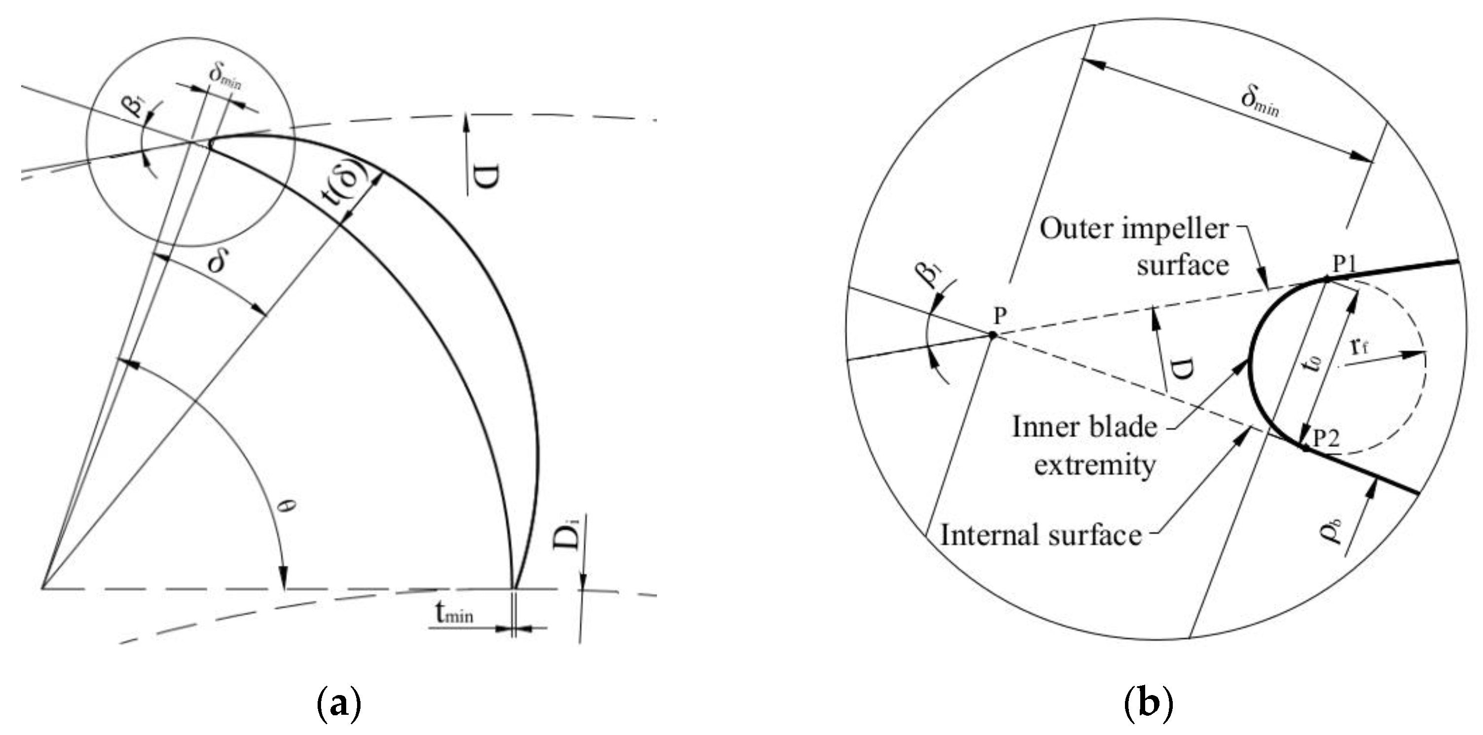
The internal surface of the blades has a circular shape, and the thickness profile is obtained by the following third-order relation [14]:
where t is the thickness along the radial direction, orthogonal to the internal surface, and δ is the angle between the radial directions at the given point and the intersection of the internal blade surface with the impeller inlet (Figure 2). According with SI, their units are m and rad, respectively.
2.2. Hydrostatic Pressure Machine (HPM)
The Hydrostatic Pressure Machine (HPM) is a novel type of hydropower converter [16] inspired by the ancient water mills. The HPM converts only the potential energy of the water flow without any transformation from the potential to the kinetic form [17].
The HPM installation inside a channel requires very little modifications of the existing infrastructure and is a good choice in water flumes with very low available head drop, like irrigation or wastewater channels, where conventional hydraulic or hydrokinetic turbines are inefficient or just too expensive because of the low power rating [17].
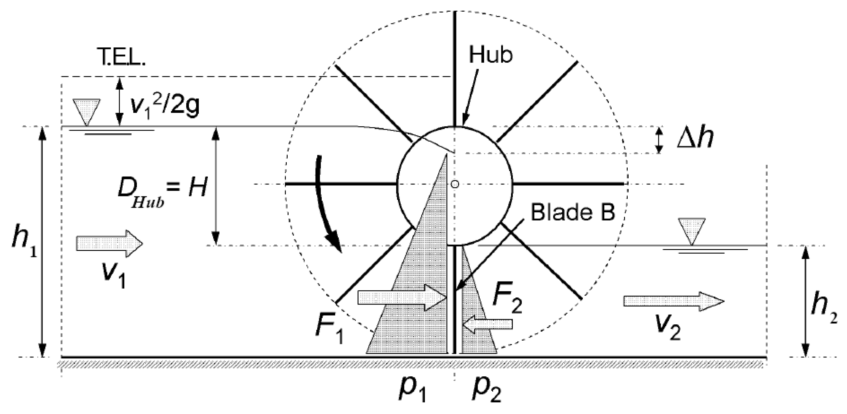
The functional scheme of the HPM is shown in Figure 3.
where:
Neglecting the momentum forces, we can assume the maximum total force on a single blade to happen when the channel rectangular cross-section is closed by the same blade. In this case, if we neglect the flux between the blade and the channel cross-section perimeters, as well as the energy dissipation next to the turbine and the resulting backwater effect, we can compute the total force as the difference between the two hydrostatic forces. The resulting torque will be equal to the total force times the radius between the turbine axis and the center of the downstream wet surface (see Figure 3).
For the continuity equation:
The mechanical power per unit width [W m−1] of the ideal machine, neglecting leakage and turbulent losses [16], is:
To account for the real working conditions, additional terms must be introduced into the previous equations for power output estimation: turbulence, acceleration and leakage losses.
Turbulence losses caused by interactions between moving blades and water are assumed to be proportional to the downstream kinetic energy according to an empirical nondimensional parameter CL = 3.0 [18].
In addition to turbulence losses, acceleration losses due to the variation of velocity from v1 to v2 when the water enters the HPM must be considered. According to [18], these losses are also proportional to the downstream kinetic energy, a nondimensional coefficient Cacc function of the two normal water depths:
The resulting power loss per unit width [W m−1] is given by:
Part of the mass flow passes through the surface between the blade and the channel cross-section perimeters. According to [16], this leakage Qleak is not constant, but is a fraction of the maximum leakage , occurring when the rotational velocity is zero. Assuming a proportionality between Δh and Qleak results in:
The maximum leakage flow-rate can be estimated as function of Qmax. Qmax is the discharge [m3 s−1] occurring when, for fixed h1 and h2 normal depths, Δh = H and the produced power is zero (from Equation (7)). This implies, from Equations (5) and (7):
has been empirically estimated through lab measurements as 0.06 Qmax [18]. Because the power is proportional to the discharge, incorporating these leakage losses multiplying the efficiency with a leakage correction factor fL [16] results in:
Finally, the hydraulic efficiency is given by:
3. Case Study: Acqua dei Corsari Wastewater Treatment Plant
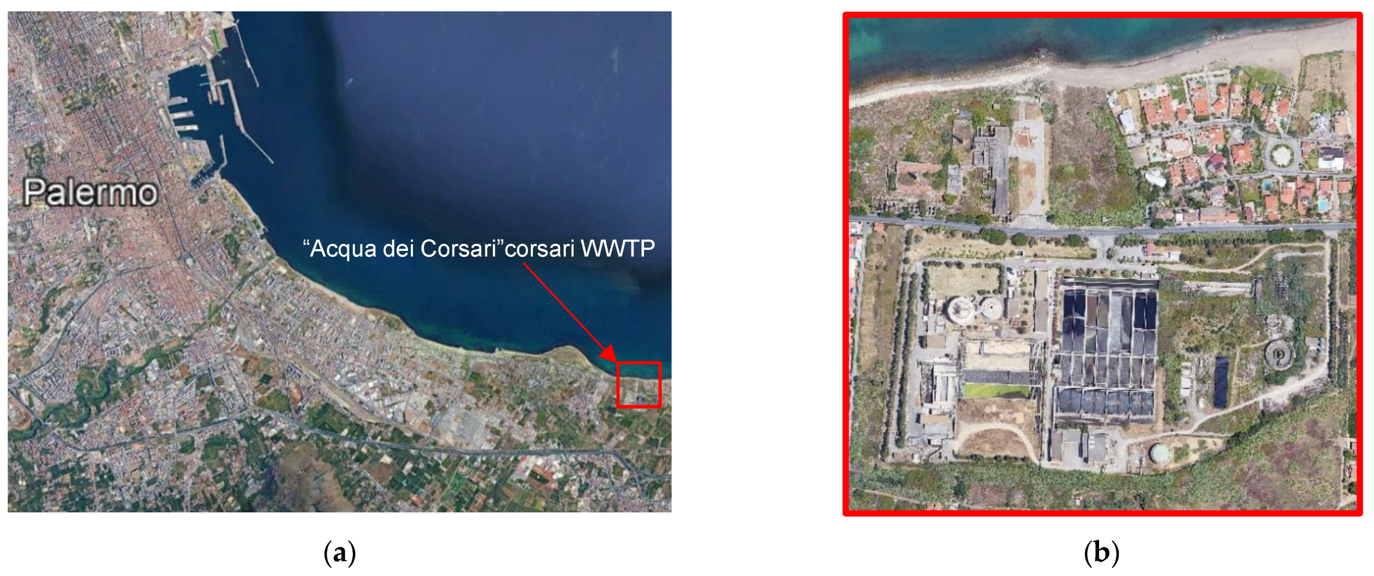
The AMAP S.p.A. is responsible for the integrated water service in 35 municipalities of the Metropolitan City of Palermo. The integrated water service also includes the transport of wastewater, its treatment and disposal. The wastewater treatment plant, named “Acqua dei Corsari”, covers an area of approximately 110,000 m2 and is located at the southeast end of the city of Palermo (Figure 4), at an average altitude of 10 m above sea level.
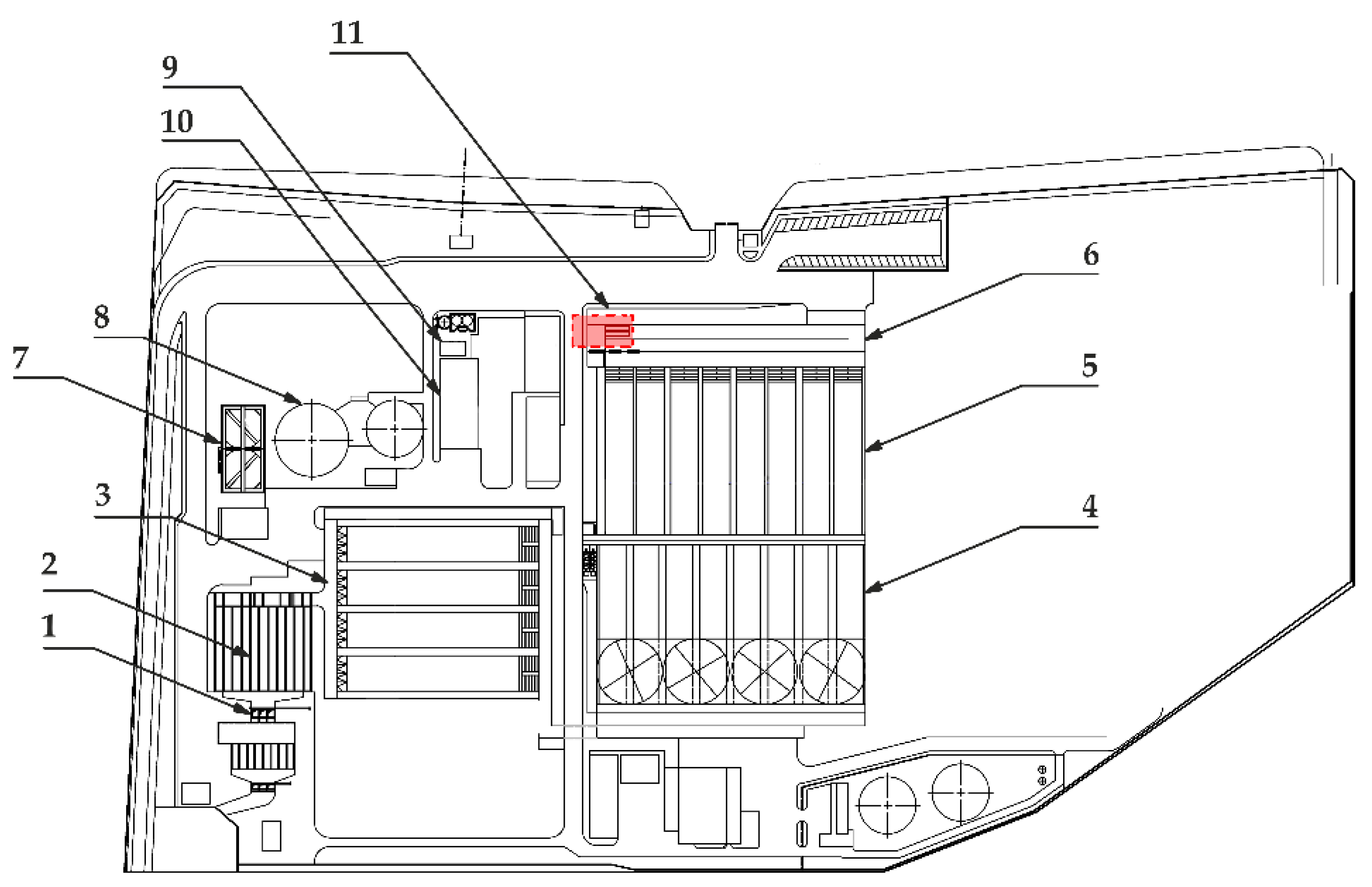
In the plant, the wastewater treatment is divided in two different steps: the water line and sludge line. The first step includes the coarse and fine grilling processes, sands and oils removal, primary sedimentation, the activated sludge process, final sedimentation and disinfection. The second step includes the prethickening, the anaerobic sludge digestion, the chemical conditioning and the sludge mechanical dewatering (Figure 5).
At the present time, the purification plant treats the wastewater produced by 320,000 equivalent inhabitants (EinH) and is expected to increase up to approximately 400,000 EinH in two years. Nowadays, the treated discharge Q is about 0.8 m3/s, but with the planned increment, it should rise up to about 1.0 m3/s. The water flow clarified from the disinfection channel (number 6 in Figure 5) crosses two rectangular weirs and reaches the discharge channel after a small head jump h1 of about 3.5 m. This discharge channel also conveys the water bypassed by the sewage treatment in the case of heavy rain events. The AMAP S.p.A. wants to reduce the energy costs linked to the purification process by recovering energy from this head jump with the installation of a hydraulic turbine.
Three different solutions are investigated: a commercial Kaplan turbine, a cross-flow-type turbine and an HPM. All these plants should be located in the area shown in Figure 5.
3.1. Kaplan Turbine Solution
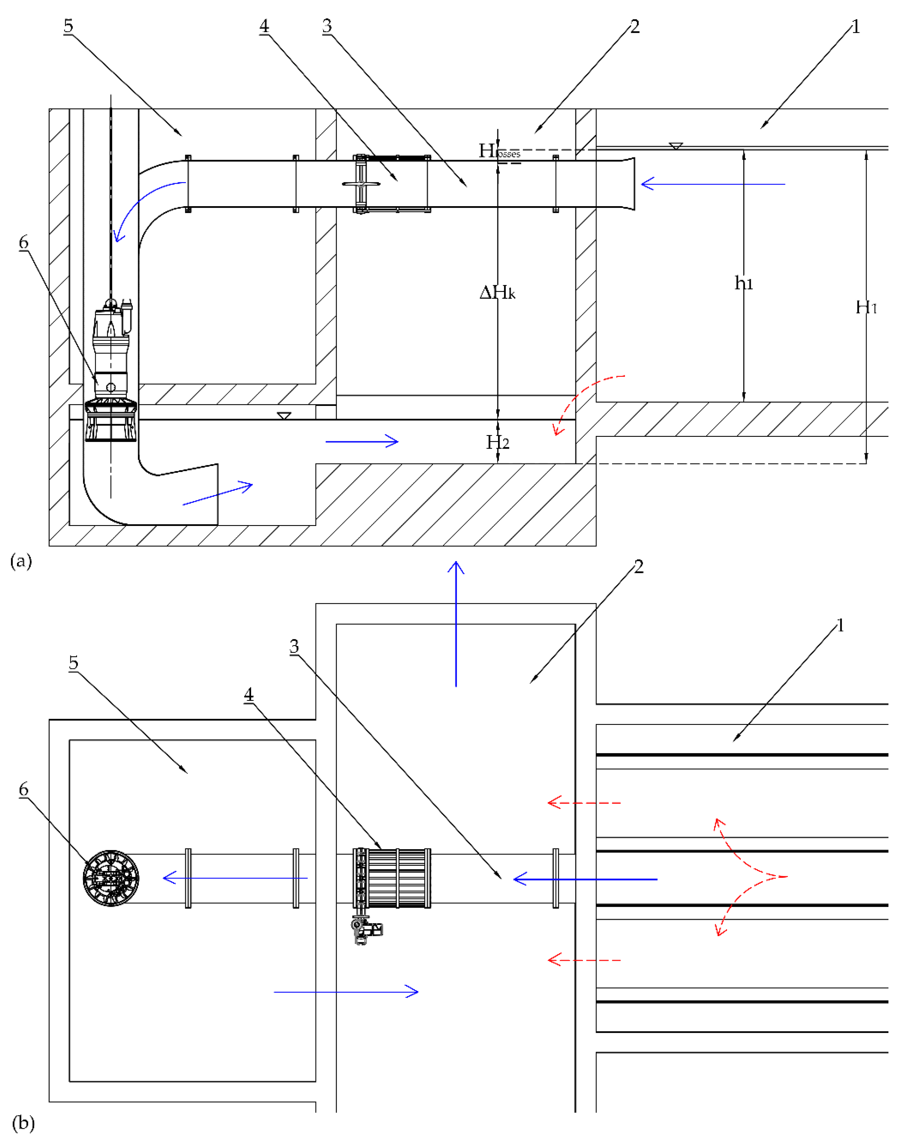
For the commercial solution, the turbine was chosen with the design parameters closest to the required ones; namely, a flow rate equal to 0.837 m3/s and a head drop equal to 3.75 m. The actual jump ΔHk = 3.75 m available for production is given by the difference between the level H1 of the inlet channel (with respect to the bed of the discharge channel) and the level H2 of the discharge channel, minus about 0.2 m of head losses Hlosses estimated in the suction pipe and in the butterfly valve, respectively marked with 3 and 4 in Figure 6. The turbine (referenced with 6) is put in a specific underground room downstream of the plant channel that should be constructed on purpose (marked 5 in Figure 6).
In case of overflow, the exceeding discharge will bypass the turbine and will reach the discharge channel through the original rectangular weirs (red dashed arrows). Observe that it is possible to cut off the turbine and restore the actual layout of the WWTP just by closing the butterfly valve, marked with number 4.
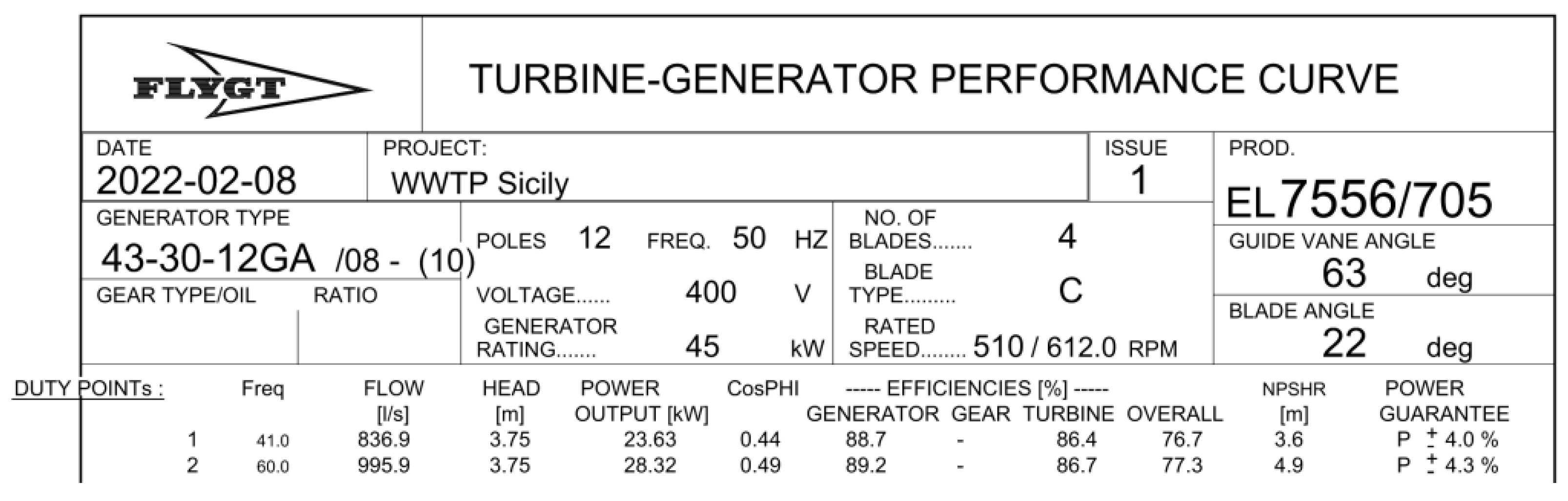
In the technical data sheet of the model (Figure 7), it is observed that the turbine attains the best efficiency equal to 86.7% for a flow rate Q = 0.996 m3/s and a head drop ΔH = 3.75 m. In the range of flow rates of the WWTP (0.8–1.0 m3/s), the efficiency reduction is lower than 1%.
3.2. Cross-Flow Turbine Solution
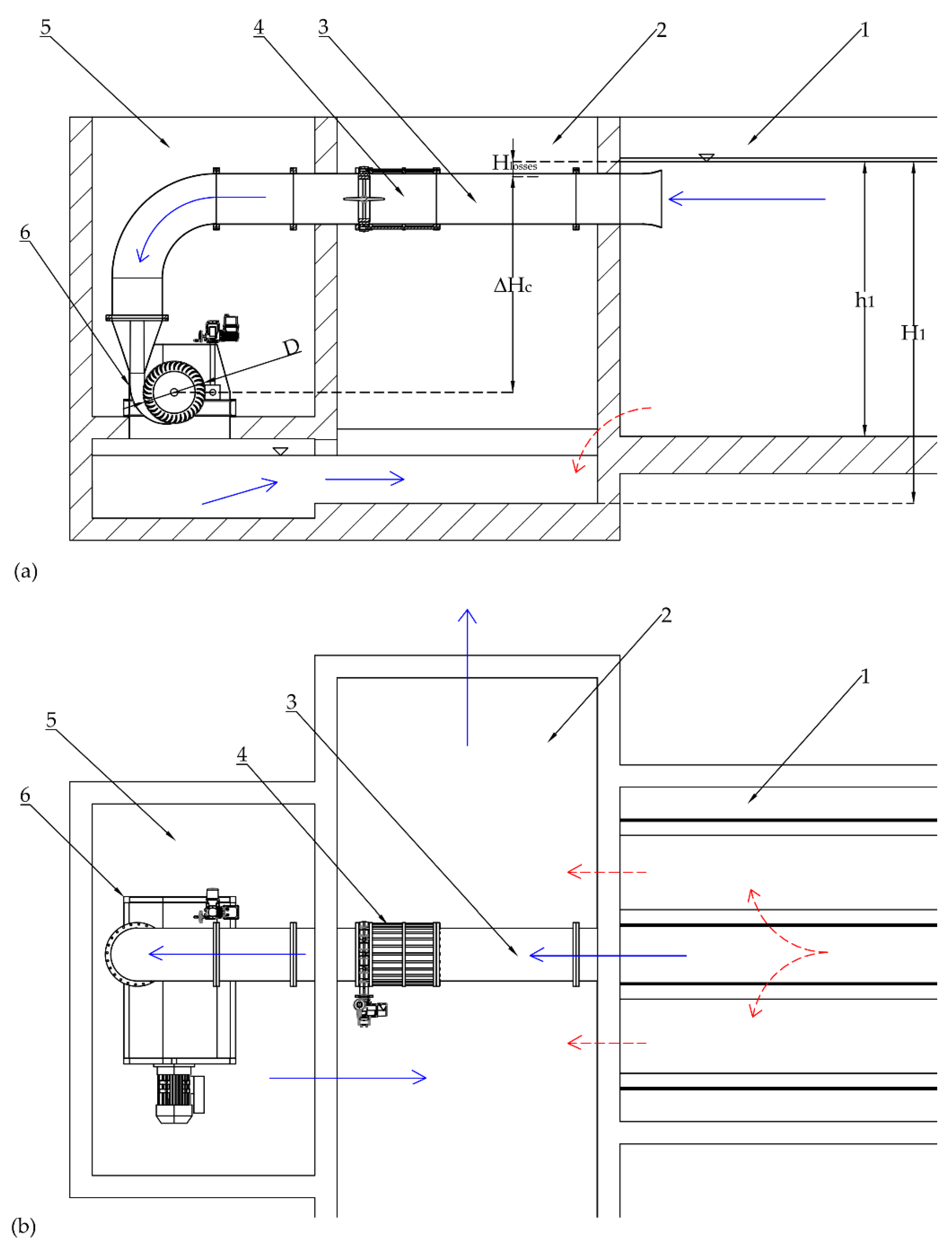
The cross-flow-type turbines could be implemented in the power recovery system (PRS) version [13,14,15], almost in the same position of the previous Kaplan turbine. The PRS turbine has an efficiency usually lower than the traditional cross-flow turbine (CFT), which has zero outflow pressure. For this reason, a CFT is preferred to allocate in the same underground room of the Kaplan, with its axis above the level of the discharge channel in order to avoid any interaction between the free surface flow in the channel and the turbine blades (Figure 8). This implies a reduction of the net head drop ΔHc from 3.75 to 2.8 m, due also to head losses Hlosses equal to 0.2 m in the suction pipe and in the butterfly valve, marked with 4 in Figure 8. Following the design criteria of the previous section, a diameter D and width W equal to 0.83 m and 0.7 m are selected, respectively, for a rotational velocity ω equal to 75 rpm.
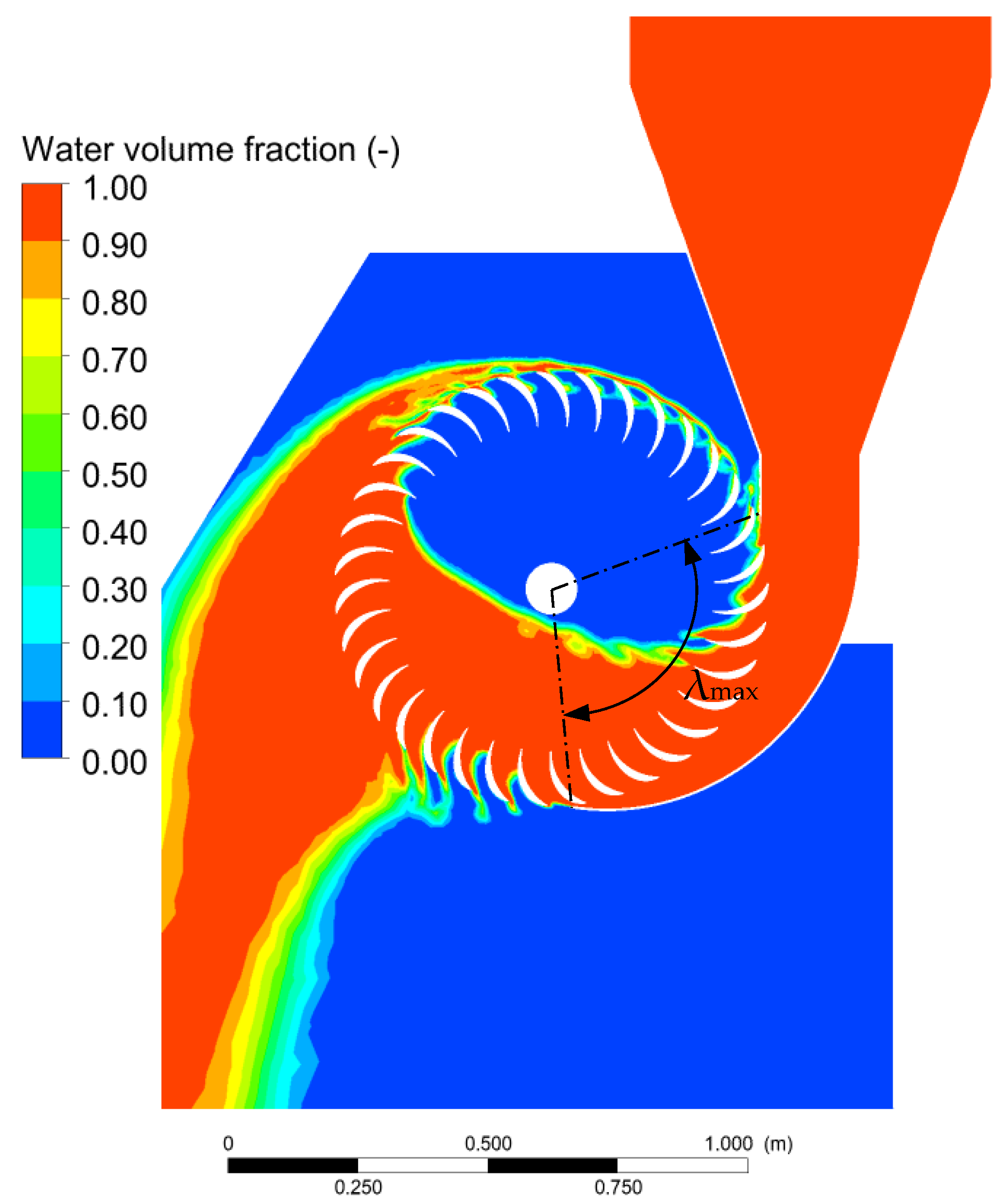
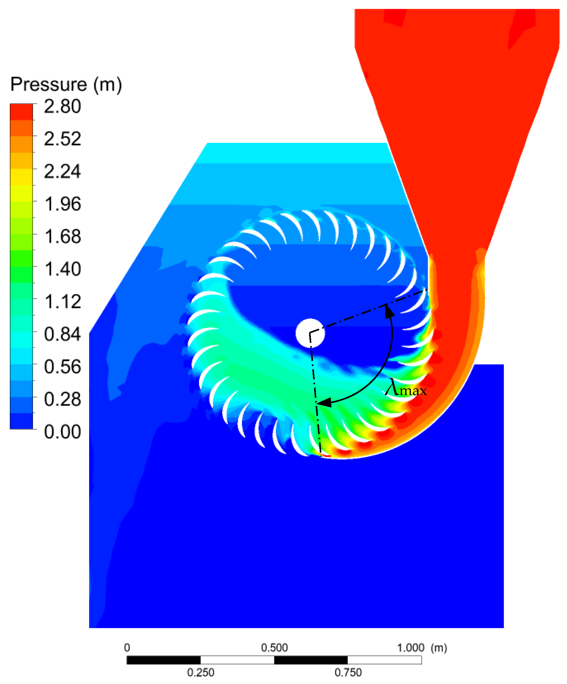
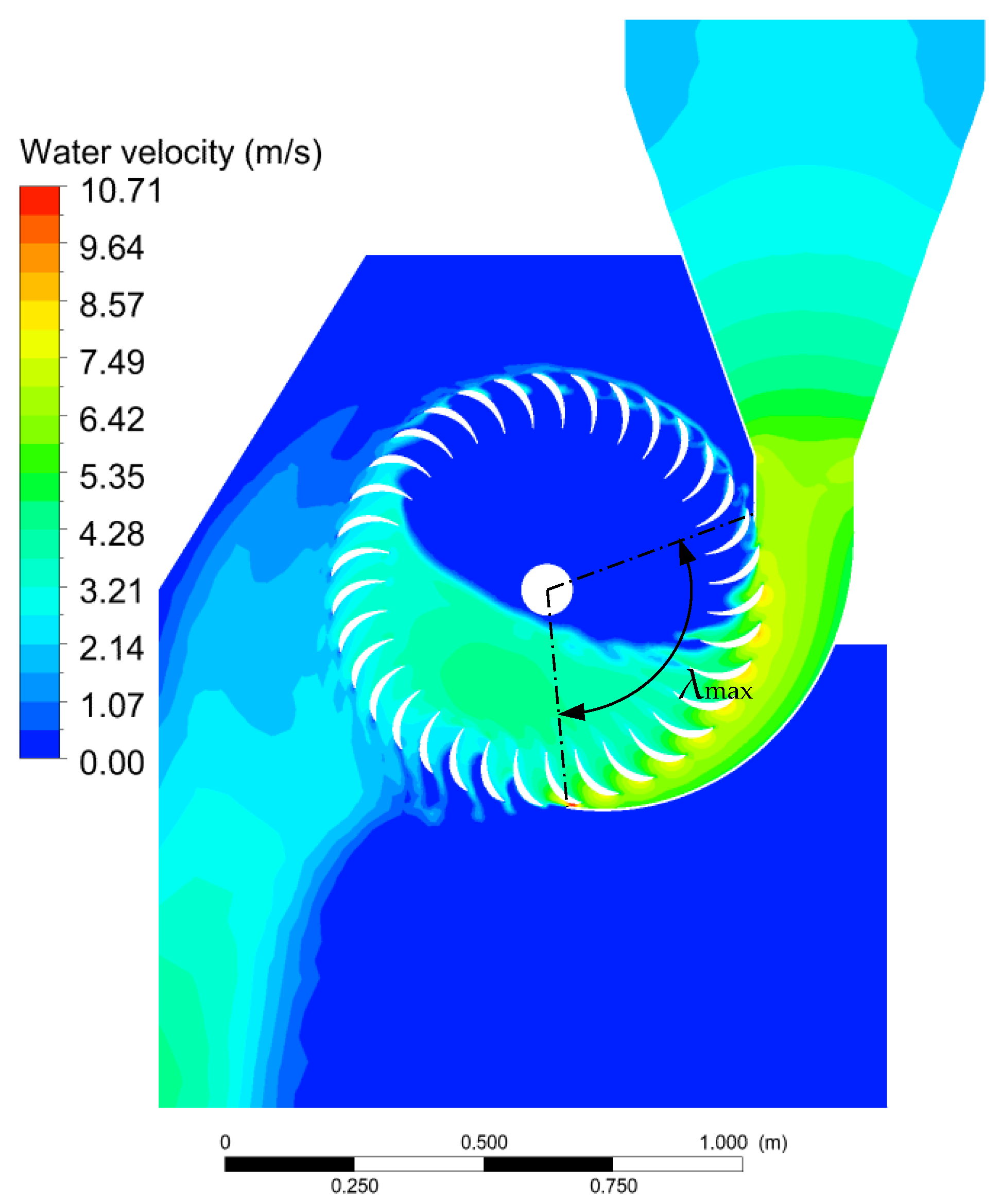
The circular section of the pipe is connected to the rectangular inlet section of the nozzle of the turbine through a special convergent. Numerical analysis has been carried out for validation by computing the efficiency and the flow rate of the turbine for a given head drop ΔHc. The turbine shows an efficiency equal to 83.5%, with a computed discharge close to design data (Q = 0.820 m3 s−1; ΔHc = 2.8 m; ω = 75 rpm; α = 15°; λmax = 100°; D = 0.84 m; W = 0.7 m). In Figure 9, Figure 10 and Figure 11, the computed volume fraction, pressure and velocity fields are shown.
3.3. HPM Turbine Solution
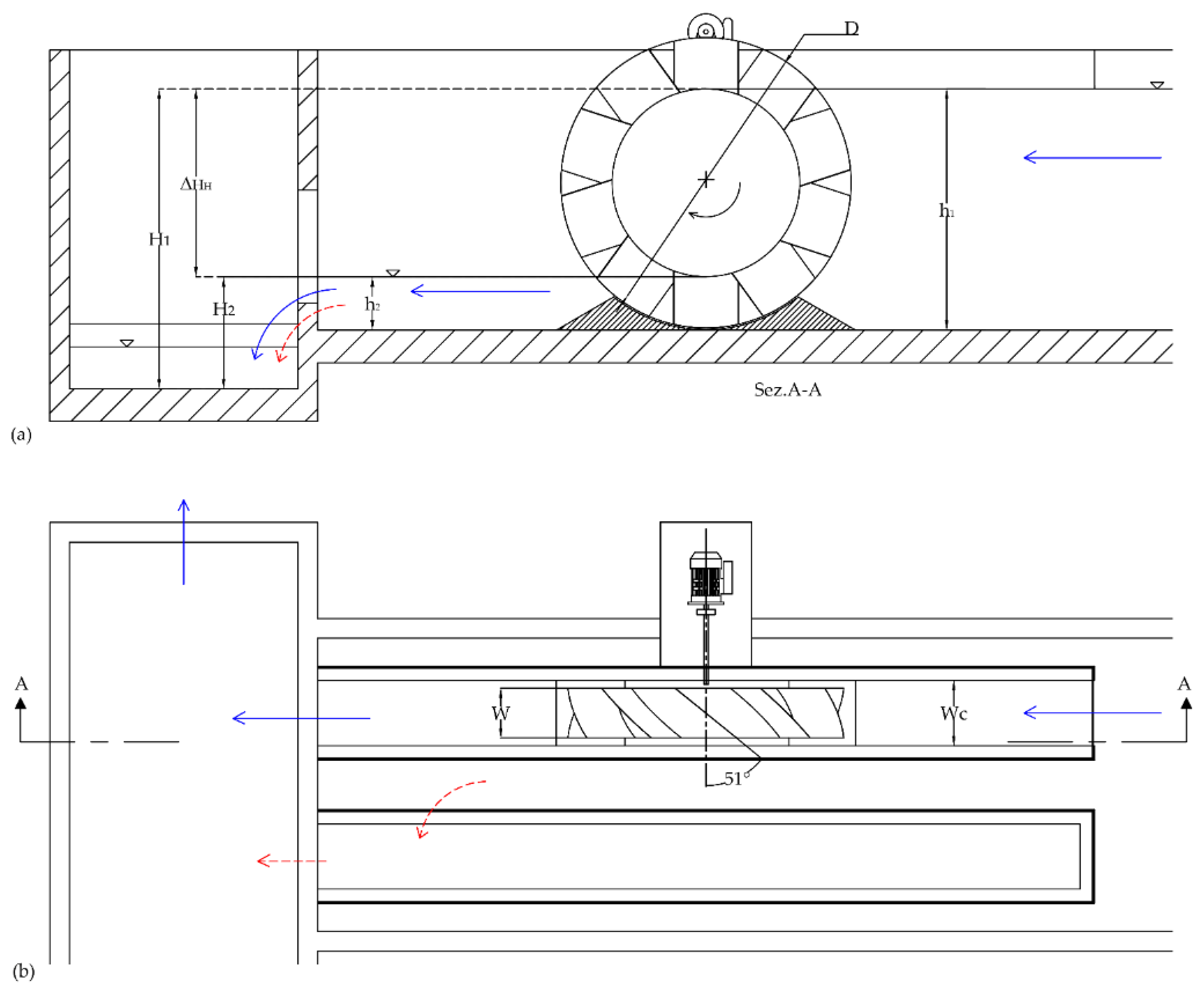
The use of the HPM turbine requires a downstream water depth greater than zero, with a water level H2 equal to the level of the inlet channel bed plus a water depth h2 = 0.75 m (Figure 12). According to the previous section, the diameter of the hub DHub is equal to ΔHH = 2.75 m, the height of the blades is equal to h2 and the outer diameter D is equal to 4.25 m. For this diameter and mass flow rate, the efficiency is given by Equation (15), which attains a maximum value ηhydro = 56% for an upstream velocity v1 equal to 0.3 m/s, corresponding to a width of the wheel W equal to 0.76 m and an angular velocity equal to 7 [rpm]. The HPM turbine is located in one of the two original rectangular weirs of a width Wc equal to 1 m, in order to respect the ratio 1:1.3 between the wheel width and width of the rectangular weir suggested in [16,18]. In case of overflow, the exceeding discharges crosses the other original rectangular weir to directly reach the discharge channel (red dashed arrows in Figure 12).
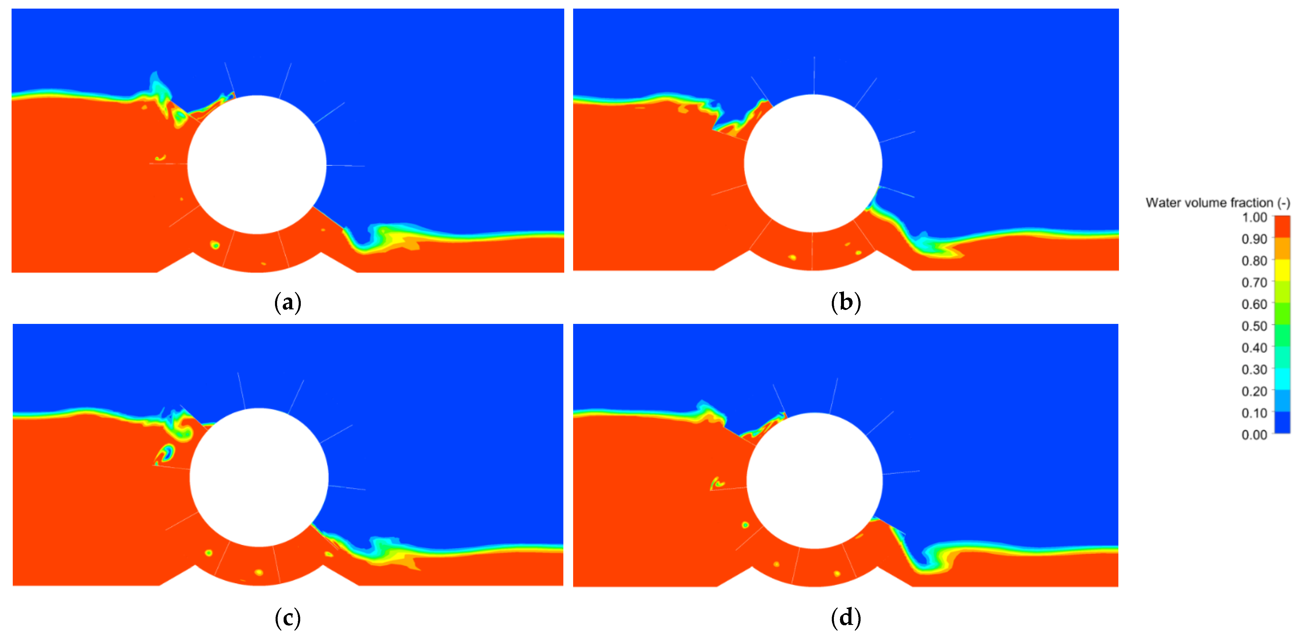
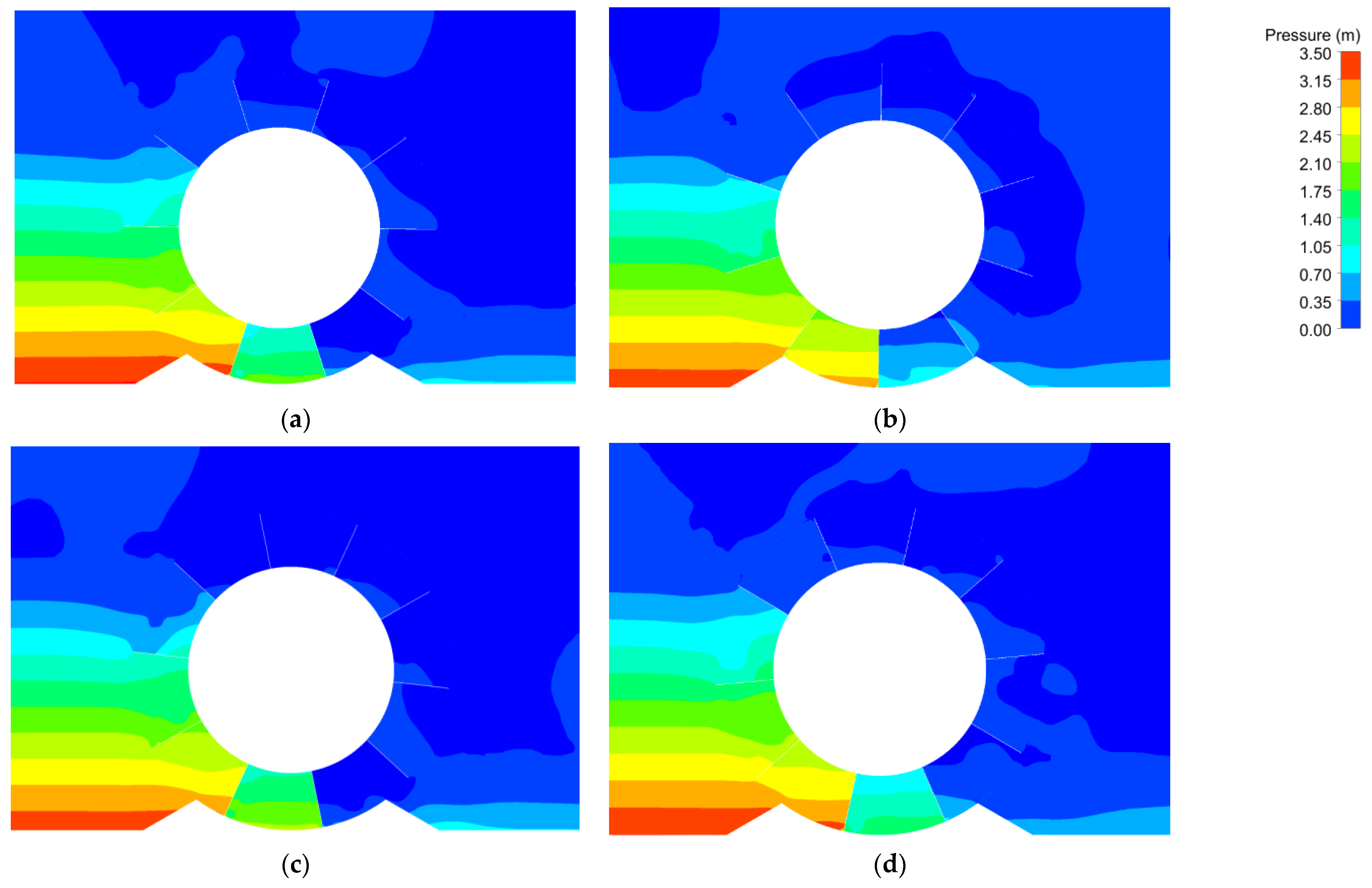
The actual orientation of each blade plane is not parallel to the rotor axis, as assumed in the previous section, but its intersection with the orthogonal plane, including the rotor axis, forms an angle of 51° with the same axis. This has been done to speed up the exit of the water from the volume confined by two sequential blades immediately after the first one attains the vertical position below the rotor axis. Numerical analysis was carried out for validation by computing the efficiency and the flow rate of the HPM for fixed h1 and h2 normal depths. The turbine shows an efficiency equal to 54.5%, with a computed discharge close to the design data (Q = 0.860 m3/s). In Figure 13 the distributions of the water volume fraction for four different simulation times t, and in Figure 14, the distributions of the pressure for four different simulation times t are shown.
4. Cost/Benefit Analysis
A final decision on whether or not a hydropower scheme should be chosen, or the selection among alternative design solutions, is generally based on the comparison of the expected costs and benefits for the lifespan of a project by means of economic analysis criteria. The effectiveness of an economic analysis as a decision tool of a hydro investor depends on the accuracy of the project cost and benefits estimated. These estimations are not always easy to reach, especially when some of the characteristics are only preliminarily defined. From the investor point of view, the only tangible revenue or benefit in a hydropower scheme is the annual income with the energy production sale. This income depends on the amount of energy produced during the hydro lifespan and on the specific conditions that rule the hydropower sector, namely the energy sale contract conditions and the tariffs policy, which are specific in each country.
For this economic analysis, the following costs are split in three main groups:
- Civil work costs: these include the cost for the required modification of the existing infrastructures: the upstream channel section for the HPM and the cost for excavation and building of a specific underground room downstream the plant channel for Kaplan and cross-flow-type turbines.
- Hydropower System costs: these include the cost of the turbine, the gearbox, electrical generator of the asynchronous type and belts if necessary. The Kaplan turbine is a commercial solution, and for the estimation of the cost, we request a quotation. For the CFT and HPM turbines, we estimated a cost of EUR 13,000 for both the gearbox and the electrical generator with a high number of the polar couples. For the CTF and HMP turbines realization, we estimated a cost, respectively, of EUR 2215/kW and EUR 2000/kW.
- Control system and installation costs: these include the cost of the control system for the regulation and management of the turbine, and the cost of installation. In the range of nominal electrical power investigated, the control system cost can be expected to be the same as that of the quotation for the Kaplan turbine for all solutions.
Table 1 summarizes the design parameters, efficiencies and costs for each energy recovery plant proposed.
In compliance with the resolution n° 280/07, the Italian Regulatory Authority for Energy [21], Networks and Environment (ARERA) sets guaranteed minimum prices pMWh for the sale of energy from renewable power generation.
For hydropower plants with a nominal power up to 1 MW and produced energy up to 250 MWh/year, the guaranteed minimum prices pMWh for the 2022 is equal to EUR 158.9/MWh [21].
Assuming the hydropower plant working 24 h a day, 330 days a year, the total producible energy over a typical year and the average cash flows for each solution are calculated (Table 1).
With the known cost of investment Ci [€] and the average cash flows Cf [€/year] for each solution, the payback period ny [years] can be calculated for a preliminary estimation of amount of time it takes to recover the cost of investments.
The cross-flow turbine plant is the solution with the shorter payback period (Table 1). A more detailed cost analysis could also analyze the ordinary and extraordinary maintenance costs, and also take into account the temporal variation of the money value.
Regarding the analysis of benefits, in the Kaplan turbine, the net available head jump is the higher of the three solutions, but the water flow in the diffuser could reach negative pressure with the risk of cavitation. This problem is not presented in the HPM and cross-flow turbines.
In the HPM, the rotational speed is very low compared with the cross-flow and Kaplan turbines, so it could be necessary to use belts and/or a gearbox with a high reduction ratio to couple the HPM with the electrical generator, with a corresponding increment of the cost and a reduction of the global efficiency. On the other hand, the HPM requires very little modifications to the existing infrastructure, and it does not require a specific underground room like the Kaplan and the cross-flow turbines.
The HPM and cross-flow turbines represent a valuable choice due their constructive simplicity in comparison with the Kaplan turbine. In Kaplan and cross-flow turbine power plants, it is possible to exclude the turbine and restore the actual layout of the plant in any moment, only by closing a butterfly valve.
A brief summary and comparison of benefits for each solution is reported in Table 2.
Depending on the system’s characteristics, objectives and economic constrains, in situ geometry available conditions are important factors that can influence the best choice for each place.
5. Conclusions
In natural or artificial channels, the best turbine for hydropower plants with low or ultra-low head jumps is usually deemed to be the Kaplan one. In the analyzed case study, it is shown that the HPM or the cross-flow turbines can also be an attractive alternative solution. The main advantage of the cross-flow turbine is its constructive simplicity against a good efficiency and a small size. The cross-flow turbines also have a very simple device for hydraulic regulation, while the Kaplan type requires the rotation of all the blades in the rotor and in the guide vane. In the case of ultra-low head jumps, the pressurized outflow of the Kaplan turbine, without the reduction of the actual head drop due to the elevation of the rotor axis with respect to the channel bed, could still provide a significant advantage with respect to the proposed competitors.
Author Contributions
Conceptualization, resources and supervision, T.T. and H.M.R.; investigation and data acquisition: C.P.; software, C.P.; methodology M.S.; writing and original draft preparation, C.P., M.S. and P.P.; formal analysis: C.A. All authors have read and agreed to the published version of the manuscript.
Funding
This research has been carried out as part of the contract between the University of Palermo and the AMAP s.p.a. water service provider, with the financial support of AMAP s.p.a. Part of this research is also supported by CERIS, IST.
Conflicts of Interest
The authors declare no conflict of interest.
References
- Molinos-Senante, M.; Maziotis, A. Evaluation of energy efficiency of wastewater treatment plants: The influence of the technology and aging factors. Appl. Energy 2022, 310, 118535. [Google Scholar] [CrossRef]
- Sabia, G.; Petta, L.; Avolio, F.; Caporossi, E. Energy saving in wastewater treatment plants: A methodology based on common key performance indicators for the evaluation of plant energy performance, classification and benchmarking. Energy Convers. Manag. 2020, 220, 113067. [Google Scholar] [CrossRef]
- Belloir, C.; Stanford, C.; Soares, A. Energy benchmarking in wastewater treatment plants: The importance of site operation and layout. Environ. Technol. 2015, 36, 260–269. [Google Scholar] [CrossRef]
- Foladori, P.; Vaccari, M.; Vitali, F. Energy audit in small wastewater treatment plants: Methodology, energy consumption indicators, and lessons learned. Water Sci. Technol. 2015, 72, 1007–1015. [Google Scholar] [CrossRef] [Green Version]
- Panepinto, D.; Fiore, S.; Zappone, M.; Genon, G.; Meucci, L. Evaluation of the energy efficiency of a large wastewater treatment plant in Italy. Appl. Energy 2016, 161, 404–411. [Google Scholar] [CrossRef]
- Gandiglio, M.; Lanzini, A.; Soto, A.; Leone, P.; Santarelli, M. Enhancing the Energy Efficiency of Wastewater Treatment Plants through Co-digestion and Fuel Cell Systems. Front. Environ. Sci. 2017, 5, 70. [Google Scholar] [CrossRef] [Green Version]
- European Environment Agency. Urban Waste Water Treatment Maps. 2015. Available online: http://www.eea.europa.eu/data-and-maps/uwwtd/interactive-maps/urban-waste-water-treatment-maps-1 (accessed on 20 January 2021).
- Eurostat. Municipal Waste Statistics—Statistics Explained. 2017. Available online: http://ec.europa.eu/eurostat/statistics-explained/index.php/Municipal_waste_statistics (accessed on 19 June 2021).
- Electric Power Research Institute and Water Research Foundation. Electricity Use and Management in the Municipal Water Supply and Wastewater Industries. 2013, pp. 1–194. Available online: http://www.epri.com/search/Pages/results.aspx?k=3002001433 (accessed on 5 January 2022).
- Shen, Y.; Linville, J.L.; Urgun-Demirtas, M.; Mintz, M.M.; Snyder, S.W. An overview of biogas production and utilization at full-scale wastewater treatment plants (WWTPs) in the United States: Challenges and opportunities towards energy-neutral WWTPs. Renew. Sustain. Energy Rev. 2015, 50, 346–362. [Google Scholar] [CrossRef] [Green Version]
- Picone, C.; Sinagra, M.; Aricò, C.; Tucciarelli, T. Numerical analysis of a new cross-flow type hydraulic turbine for high head and low flow rate. Eng. Appl. Comput. Fluid Mech. 2021, 15, 1491–1507. [Google Scholar] [CrossRef]
- Sammartano, V.; Morreale, G.; Sinagra, M.; Tucciarelli, T. Numerical and experimental investigation of a cross-flow water turbine. J. Hydraul. Res. 2016, 54, 321–331. [Google Scholar] [CrossRef] [Green Version]
- Sinagra, M.; Sammartano, V.; Morreale, G.; Tucciarelli, T. A new device for pressure control and energy recovery in water distribution networks. Water 2017, 9, 309. [Google Scholar] [CrossRef] [Green Version]
- Sinagra, M.; Picone, C.; Aricò, C.; Pantano, A.; Tucciarelli, T.; Hannachi, M.; Driss, Z. Impeller Optimization in Crossflow Hydraulic Turbines. Water 2021, 13, 313. [Google Scholar] [CrossRef]
- Sammartano, V.; Sinagra, M.; Filianoti, P.; Tucciarelli, T. A Banki-Michell turbine for in-line hydropower systems. J. Hydraul. Res. 2017, 55, 686–694. [Google Scholar] [CrossRef]
- Senior, J.; Saenger, N.; Müller, G. New hydropower converters for very low-head differences. J. Hydraul. Res. 2010, 48, 703–714. [Google Scholar] [CrossRef]
- Pienika, R.; Usera, G.; Ramos, H.M. Simulation of a Hydrostatic Pressure Machine with Caffa3d Solver: Numerical Model Characterization and Evaluation. Water 2020, 12, 2419. [Google Scholar] [CrossRef]
- Schneider, S.; Müller, G.; Saenger, N. HYLOW Project Report: Converter Technology Development—HPM and HPC; Internal Task Report 2.3; EU: Damstadt, Germany, 2012. [Google Scholar]
- Senior, J.; Wiemann, P.; Müller, G. The Rotary Hydraulic Pressure Machine for Very Low HEAD Hydropower Sites. Available online: http://www.hylow.eu/knowledge/all-download-documents/ (accessed on 7 August 2020).
- Sinagra, M.; Sammartano, V.; Aricò, C.; Collura, A. Experimental and Numerical Analysis of a Cross-Flow Turbine. J. Hydraul. Eng. 2016, 142, 1. [Google Scholar] [CrossRef]
- Italian Regulatory Authority for Energy, Networks and Environment (ARERA). Prezzi Minimi Garantiti per l’anno 2022. Available online: https://www.arera.it/it/comunicati/22/220118.htm (accessed on 18 January 2022).
Figure 1.
Cross-flow turbine: (a) Section view on symmetry plan of the turbine; (b) Side view. D and W are diameter and width of the runner, V the runner velocity at the inlet surface, ω the runner rotational velocity, α is the velocity inlet angle with respect to the tangent direction and λmax the central angle of the inlet surface.

Figure 2.
(a) Blade profile; (b) Tangent condition of external end [14]. D and Di are the outer and inner diameter of the runner, β1 is the relative velocity inlet angle with respect to the tangent direction in P, rb and θ are the radius and the central angle of internal surface of the blade, respectively, t is the thickness along the radial direction, orthogonal to the internal surface and δ is the angle between the radial directions at the given point and the intersection of the internal blade surface with the runner inlet. t0 is the thickness corresponding at δmin, rf the radius of the fillet of the tip of the blade, the tip of the blade is tangent in point P1 to the cubic spline profile of the external surface, and in P2 to the circular profile of the internal surface, and tmin is the thickness located at the extremity (δ = θ).

Figure 3.
Functional scheme of the HPM, where: T.E.L. is total energy level [m]; h1 is the water depth of the upstream channel [m]; h2 is the water depth of the downstream channel [m]; H is the head difference [m]; v1 is the water upstream velocity [m s−1]; v2 is the water downstream velocity [m s−1]; F1 is the force acting on the blade per unit width [N m−1]; F2 is the reaction force on the blade per unit width [N m−1] [17].

Figure 4.
Aerial view of: (a) Metropolitan City of Palermo; (b) “Acqua dei Corsari” WWTP.

Figure 5.
Acqua dei Corsari” WWTP plant, where: 1. Grilling processes; 2. Sands and oils removal; 3. Primary sedimentation; 4. Activated sludge process; 5. Final sedimentation; 6. Disinfection; 7. Prethickening; 8. Anaerobic sludge digestion; 9. Chemical conditioning; 10. Sludge mechanical dewatering; 11. Low-head hydropower.

Figure 6.
(a) Section and (b) planimetric view of the Kaplan type turbine plant where: 1. Inlet channel; 2. Discharge channel; 3. Suction pipe; 4. Butterfly valve; 5. Underground room; 6. Kaplan turbine. The actual jump is ΔHK = 3.75 m; h1 = 3.5 m is the level of the inlet channel; H1 = 4.3 m is the level of the inlet channel (with respect to the bed of the discharge channel); H2 = 0.35 m is the level of the dis-charge channel; Hlosses is head losses estimated about 0.2 m in the suction pipe and in the butterfly valve, respectively marked with 3 and 4.

Figure 7.
Technical data sheet of Kaplan type turbine plant.

Figure 8.
(a) Section and (b) planimetric view of cross-flow-type turbine plant, where: 1. Inlet channel; 2. Discharge channel; 3. Suction pipe; 4. Butterfly valve; 5. Underground room; 6. Cross-flow turbine. The actual jump is ΔHc = 2.8 m; h1 = 3.5 m is the level of the inlet channel; H1 = 4.3 m is the level of the inlet channel (with respect to the bed of the discharge channel); Hlosses is head losses estimated about 0.2 m in the suction pipe and in the butterfly valve, respectively marked with 3 and 4; D = 0.84 m is the outer diameter of the runner.

Figure 9.
Water volume fraction contours for cross-flow-type turbine (λmax = 100°).

Figure 10.
Pressure contours for cross-flow-type turbine (λmax = 100°).

Figure 11.
Water velocity field contours for cross-flow-type turbine (λmax = 100°).

Figure 12.
(a) Section and (b) planimetric view of HPM plant: The actual jump is ΔHH = 2.75 m; h1 = 3.5 m and h2 = 0.75 are the level of the inlet channel in the sections before and after the wheel; H1 = 4.3 m is the level of the inlet channel (with respect to the bed of the discharge channel); H2 is the level of the discharge channel; D = 4.25 m is the outer diameter of the runner; W = 0.76 m is the width of the runner; Wc = 1.0 m is the width of the channel. The angle between the rotor axis and the intersection between the blade plane and its orthogonal one, including the axis, is 51°.

Figure 13.
Water volume fraction contours for HPM: (a) t = 18 s; (b) t = 21 s; (c) t = 23 s; (d) t = 25 s.
Figure 13.
Water volume fraction contours for HPM: (a) t = 18 s; (b) t = 21 s; (c) t = 23 s; (d) t = 25 s.

Figure 14.
Pressure contours for HPM: (a) t = 18 s; (b) t = 21 s; (c) t = 23 s; (d) t = 25 s.


Table 1.
Comparison of electrical energy recovery economic indicators.
| Parameters | Kaplan | Cross-Flow | HPM |
|---|---|---|---|
| Design Head ΔH [m] | 3.75 | 2.8 | 2.75 |
| Design Flow rate Q [m3/s] | 0.837 | 0.820 | 0.860 |
| Hydraulic Efficiency | 0.864 | 0.835 | 0.545 |
| Gearbox/belts/generator efficiency | 0.887 | 0.887 | 0.870 * |
| Global efficiency | 0.766 | 0.741 | 0.474 |
| Nominal Power (PElectrical) [kW] | 23.6 | 16.7 | 11.0 |
| Civil works [€] | 20,000 | 20,000 | 5000 |
| Hydropower System [€] | 165,000 | 50,000 | 35,000 |
| Control system and installation [€] | 40,000 | 40,000 | 40,000 |
| Total (Ci) [€] | 225,000 | 110,000 | 80,000 |
| Specific cost [€/kW installed] | 9534 | 6587 | 7273 |
| Total producible energy [MWh] | 186.912 | 132.264 | 87.120 |
| Average cash flows (Cf) [€/year] | 29,700 | 21,017 | 13,843 |
| Payback period (ny) [year] | 7.6 | 5.2 | 5.8 |
* According to [19].
Table 2.
Benefit comparison of solutions.
| Kaplan | Cross-Flow | HPM | |
|---|---|---|---|
| Net available head jump | ✔ | ✘ | ✘ |
| Risk of cavitation | ✘ | ✔ | ✔ |
| Rotational velocity | ✔ | ✔ | ✘ |
| Hydraulic Efficiency > 80% | ✔ | ✔ | ✘ |
| Payback period | ✘ | ✔ | ✔ |
| Nominal power | ✔ | ✘ | ✘ |
| Building a specific underground room | ✘ | ✘ | ✔ |
| Constructive simplicity of the turbine | ✘ | ✔ | ✔ |
| Possibility to exclude turbine and restore the actual WWTP layout | ✔ | ✔ | ✘ |
Publisher’s Note: MDPI stays neutral with regard to jurisdictional claims in published maps and institutional affiliations. |
© 2022 by the authors. Licensee MDPI, Basel, Switzerland. This article is an open access article distributed under the terms and conditions of the Creative Commons Attribution (CC BY) license (https://creativecommons.org/licenses/by/4.0/).
Share and Cite
MDPI and ACS Style
Sinagra, M.; Picone, C.; Picone, P.; Aricò, C.; Tucciarelli, T.; Ramos, H.M. Low-Head Hydropower for Energy Recovery in Wastewater Systems. Water 2022, 14, 1649. https://0-doi-org.brum.beds.ac.uk/10.3390/w14101649
AMA Style
Sinagra M, Picone C, Picone P, Aricò C, Tucciarelli T, Ramos HM. Low-Head Hydropower for Energy Recovery in Wastewater Systems. Water. 2022; 14(10):1649. https://0-doi-org.brum.beds.ac.uk/10.3390/w14101649
Chicago/Turabian StyleSinagra, Marco, Calogero Picone, Paolo Picone, Costanza Aricò, Tullio Tucciarelli, and Helena M. Ramos. 2022. "Low-Head Hydropower for Energy Recovery in Wastewater Systems" Water 14, no. 10: 1649. https://0-doi-org.brum.beds.ac.uk/10.3390/w14101649
Note that from the first issue of 2016, this journal uses article numbers instead of page numbers. See further details here.