
Interaction between Strong Sound Waves and Aerosol Droplets: Numerical Simulation


1
College of Water Resources & Civil Engineering, China Agricultural University, Beijing 100083, China
2
Department of Engineering Mechanics, Zhejiang University, Hangzhou 310027, China
3
State Key Laboratory of Hydroscience & Engineering, Tsinghua University, Beijing 100084, China
4
State Key Laboratory of Plateau Ecology and Agriculture, Qinghai University, Xining 810016, China
*
Authors to whom correspondence should be addressed.
Water 2022, 14(10), 1661; https://0-doi-org.brum.beds.ac.uk/10.3390/w14101661
Submission received: 6 April 2022
/
Revised: 13 May 2022
/
Accepted: 16 May 2022
/
Published: 23 May 2022
(This article belongs to the Special Issue Atmospheric Water Resources Exploitation and Utilization)
Abstract
:In this study, we attempted to eliminate atmospheric fog and aerosol particles by strong sound waves. The action of sound waves created an air disturbance, and the oscillation of the local air caused the micron-sized aerosol droplet particles to move. To provide guidance of the characteristics of the effective sound waves, this study numerically simulated aerosol droplet agglomeration under the action of sound waves, which was solved by coupling computational fluid dynamics (CFD) and discrete element methods (DEMs) as a typical two-phase flow problem in this study. The movements of aerosol droplet particles were simulated, as well as their agglomeration. The evolution process of the average particle size and the number of multimers were obtained, and the influence of different sound frequencies, sound pressure level (SPL), and particle spacing on agglomeration were studied. It was found that the promotion effect of low-frequency sound waves on aerosol droplet agglomeration was significantly higher than that of high-frequency sound waves, and the sound wave promotion effect of high SPLs was better than that of low SPL. In addition, the concept of the average agglomeration time required to quantify the acoustic agglomeration speed was proposed, and it was found to be positively correlated with sound frequency and particle spacing, while being negatively correlated with SPL.
1. Introduction
Relative oscillating motion between particles can be caused by strong sound waves, resulting in the increasing of collision probability and the forming of particles with larger diameters, known as acoustic agglomeration [1,2] After firstly reported by Patterson and Cawood in 1931 [3], the phenomena of acoustic agglomeration have been widely applied in industrial dust removal [4], air purification [5], precipitation enhancement [6], and other fields.
There have been various theoretical explanations on the mechanism of acoustic agglomeration, mainly including: orthokinetic interaction [7], hydrodynamic interaction [8], acoustic streaming [9], and Brownian agglomeration [10]. However, due to the complexity of the dynamic process of acoustic agglomeration, the results of these theoretical studies are insufficient or even contradictory [11]. Some scholars attempt to investigate the mechanism from the perspective of the force exerted on the particles in the sound field. Knoop and Fritsching [12] compared acoustic force with van der Waals force and the interparticle adhesive force under liquid bridging. Sepehrirahnama et al. [13] numerically calculated the acoustic wave force for multiple spheres in viscous fluids. Li et al. [14] analysed the force condition of the particles in the oscillating flow field. Jia et al. [15] solved the complex nonlinear differential equation to show the movement characteristics of cloud droplets under the action of sound waves.
In addition to the theoretical research, experimental studies have also been performed to explain or exploit the effect of acoustic agglomeration, which can be classified into two categories: the physical experiments and the numerical experiments. Zhou et al. [16] demonstrated that the acoustically induced agglomeration effect can enhance the dust removal efficiency using a combination of an acoustic agglomeration experiment system and traditional dust removal device. Amiri et al. [17] used acoustic particle adjustment devices to study the impact of the frequency and sound pressure level (SPL) on the condensation and precipitation of PM2.5 aerosols. Sadighzadeh et al. [18] examined the use of a sound field in removing sulphur-assisted mist in an airflow under high SPL conditions. Cao et al. [19] designed a novel microscopic experiment to visually present the growth process of micro-droplets under the action of sound waves and obtained the critical values of sound characteristics for obvious acoustic agglomeration of droplets. Qiu et al. [20] set up a cloud chamber experimental device to simulate the effect of the sound waves on the cloud droplets under warm cloud conditions, and concluded that under a constant SPL, the sound wave with a frequency ranging from 50 to 65 Hz led to a higher agglomeration of the cloud droplets.
Along with the rapid development of computing capacity, numerical models have been proposed, such as population balance modelling and Discrete Element Method (DEM). Markauskas et al. [21] modified the standard discrete element method, and performed a numerical modelling of the agglomeration of two identical particles in a strong acoustic field. Kacianauskas et al. [22] found, in DEM analysis, that acoustically induced motion is not affected by gravity. Maknickas et al. [8] further investigated hydrodynamic effects in acoustically induced attractive motion of micron-sized particles in a three-dimensional system. Shi et al. [23] developed a coupled Computational Fluid Dynamics (CFD) and DEM model to investigate acoustic agglomeration performance of aerosol droplets in a high-temperature and high-pressure environment by the COMSOL Multiphysics software, which focused on the action of acoustic waves of high-frequency and super-high SPL (as high as 170 dB) under an unconventional condition on the aerosols with unique particle size (10 μm).
To provide a more realistic guidance for the application of sound waves to the fog and aerosol removal and precipitation modification under the natural state, this study established a CFD-DEM model with the introduction of an elastic coefficient, which was found to have a great impact on the simulation. It was proposed in this study that sound waves caused periodic changes in the pressure and flow velocity of sound fields. On one hand, they directly affected the interaction between the air medium and the particles; on the other hand, they indirectly affected the turbulent structure of the air medium, thereby realizing the effect of acoustic agglomeration. A typical two-phase flow system formed by the oscillating air flow field and the aerosol droplet particles caused by sound waves was numerically simulated to explore the acoustic agglomeration rule of aerosol droplets. The fluid phase was simulated using the CFD method, the particle phase was simulated using the DEM method, and the coupling between CFD-DEM was realized by information exchange between the two phases. In the simulation, the input parameters were changed to analyse the influence of different frequencies, SPLs, particle spacing, and other factors on the agglomeration of particles.
According to the simulated results, the variation process of the acoustic agglomeration described by the average particle size, the number of multimers, the average agglomeration time, and other variables were analysed [24] to verify the phenomenon of acoustic agglomeration, as well as to explore the effect of different sound waves on the agglomeration. As a series of experimental and theoretical studies [14,15,19,20] have confirmed that the sound waves with low frequency (<100 Hz) can promote the motion of the aerosol droplets effectively, the agglomeration behaviour of the aerosol droplets under the action of sound waves with low frequency was simulated in this study, and investigations were performed to determine the mechanical mechanism and law of sound waves to promote the motion of aerosol droplet particles.
2. Methodology
2.1. Physics Definition
A two-phase flow system is formed if fluid and particles coexist in the same space, which is a typical complex system ubiquitous in both natural and man-made states.
The aerosol droplet agglomeration under the action of strong sound waves can be regarded as a two-phase flow system. The sound wave triggers a change in the air pressure, and thus causes the air to oscillate, which can be regarded as the fluid phase. The aerosol droplet particles suspended in the air can be regarded as the particle phase. The fluid and the particles exist in the same space, where the fluid affects the movement of the particles; meanwhile, the existence of the particles has a reaction to the flow field. Thus, the two phases are coupled to form a two-phase flow system. The key to simulating the aerosol droplets’ motion under the action of sound waves is to solve this two-phase flow problem.
2.2. Mechanical Modelling
The models that are applicable to two-phase flow systems can be classified into two categories: (1) the Euler–Eulerian models, which treat the solid phase as a pseudo fluid, while regarding the solid phase and the fluid phase as continuous and interpenetrative media, and (2) the Euler–Lagrangian models, which treat fluid as a continuous phase and particles as a discrete phase; the motion of the fluid is studied in Euler coordinates and the motion of the particles is examined in Lagrangian coordinates. In this study, the Euler-Lagrangian model based on CFD-DEM [25] was applied.
Defelice [26] studied the particle system by performing empirical fitting, and proposed a drag force model for particles with a diameter of dpi considering the fluid motion and particle void fraction, as shown in Equations (1)–(4).
where is the drag force on the particle, is the fluid velocity, is the fluid density, is the particle velocity, is void fraction of the fluid cell j, the void fraction function corrects the influence of other particles, the index χ takes into account the influence of different flow regimes, and the subscript j represents the fluid grid where the ith particle exists, indicates the drag coefficient without considering the resistance, is the Reynolds number, and μs is the shear viscosity.
The suspended aerosol droplets were mainly affected by the wind in the horizontal direction, and by the gravity and the air lifting force in the vertical direction. Under the action of sound waves, the aerosol droplets were no longer balanced in the forces and began to move. The main concern of the aerosol droplet was the particles’ agglomeration to form larger multimers and settling, so the model was built up in the vertical direction. Owing to the balance between the initial gravity and air lift, neither of these two forces were introduced in modelling.
The effect of the travelling wave was equivalent to the periodic change of the air physics field caused by the action of sound waves, which was simulated by the oscillation of a box in this study, i.e., the upwards and downwards oscillation of the box was used to simulate the sound wave in the vertical direction. The air medium existed inside the box, and it only flowed out in one direction at the upper and lower boundaries. When the box moved upward, the air flow cannot flow out of the lower boundary, as the air nearby was compressed, and thus the air pressure changed, and vice versa. As the box moved continuously, the internal air pressure changed continuously, resulting in a periodic flow field that simulated the effect of sound waves.
Real aerosol droplets have irregular shapes, and there is limited research in this area. Meanwhile, for a stable suspended aerosol droplet particle, the shape was close to a sphere owing to small variations in the velocity. Therefore, the particles were simplified as spherical particles having different sizes in the simulation. In addition, the aerosol droplets will be deformed in the actual agglomeration when small particles aggregate into one large particle, which was simulated by a multimer in the modelling with a volume equivalent to the sum of the volumes of all the small particles. The diameter of a large spherical particle can be calculated accordingly, and was called the calculated average particle size. The calculated average particle size of the multimer was used to represent the equivalent particle size of the aerosol droplet particle after agglomeration. After the simplifications above, the aerosol droplet particles were represented by a spherical rigid body with a viscous surface. In actual coagulation, the droplets did not separate once they agglomerated to one large particle, and for the simulation, a surface energy was applied to the particles. Those small particles in the multimer have to overcome such a surface energy to separate from each other, and should be sufficiently large, while also ensuring the computational stability.
A numerical mechanical model was established based on the analysis and processing above. Figure 1 shows a schematic of the proposed model. The calculation domain was defined within the model, as indicated by the black box in Figure 1a. The box in the calculation domain represented by the green frame in Figure 1a was also defined, and performed simple harmonic motion in the vertical direction. The amplitude and frequency of the displacement can be defined according to the simulation requirements. Air was introduced into the calculation domain, which oscillated and propagated owing to the simple harmonic vibration of the box as the simulation of the sound wave. A formation domain was defined inside the box, and the aerosol droplet particles were generated only in this formation domain, as shown in Figure 1b. This formation domain was a virtual area that was only used to define the particle generation range, and it had no effect on the movement of the particles. The parameters of the particles were set according to the rigid sphere assumption.
To distinguish between particles with different sizes, different colours were used in Figure 1b. The purple particles represent particles with a diameter of 10 μm, the brown particles represent those with a diameter of 20 μm, and the blue particles represent those with a diameter of 30 μm. All particles were randomly generated within the generation domain, and they did not collide with each other.
The model parameters were mainly classified into three categories: particle-relevant, flow field-relevant, and box-relevant parameters. In the parameter setting, the characteristics of actual aerosol droplet particles under the action of sound waves, the purpose of the numerical simulation, and the computational capabilities of the PC were extensively considered to determine the calculation domain.
A particle swarm is a simulation of aerosol droplet particles that is simplified to spherical rigid bodies. The typical particle size of a cloud droplet was 20 μm, which was set as the median diameter of the particles. Within the set calculation domain, particles with diameters of 10 μm, 20 μm, and 30 μm were randomly generated in the generation domain with amounts of 120, 240, and 120, respectively. The initial average particle spacing was set to 20 μm, and the density of the particles was the same as that of water, i.e., 1×10³ kg/m3. As only the forces in the vertical direction were considered, and owing to the balance between gravity and the lifting force, particles were only affected by the flow field generated by the sound waves. The initial flow velocity was set to 0, and the initial pressure in the whole calculation domain was the standard atmospheric pressure, i.e., 101,325 Pa. The thermal process of low-frequency sound waves acting on the air can be regarded as an isothermal process, and the temperature was constant at 293 K in the simulation. The amplitude and frequency of the vibration of the box were set according to the requirements.
2.3. Determination of Box-Relevant Parameters
The amplitude and frequency of the box vibration determined the intensity of its disturbance to the air. Inputting a group of amplitudes and frequencies to the model, the pressure change in each fluid grid can be derived by performing calculations, as well as the average sound pressure level (SPL). In this study, Equation (5) was used to calculate SPL.
where ∆p is the variation of air pressure, and is the reference acoustic pressure, which is 2 × 10⁻⁵ Pain air.
In the calculation, two fluid grids with larger distances were selected to illustrate the pressure fluctuation map in order to derive ∆p. If these two values of ∆p agree, the SPL in the calculation domain is considered to be uniform, and the average of these two ∆p values is used to represent the SPL in the simulation. Table 1 shows the SPL under different sound frequency conditions for particles of different sizes, and Table 2 shows a group of sound frequency conditions and particle sizes corresponding to an SPL of approximately 100 dB, which can be used in the simulation.
3. Parameter Calibration
Before the numerical simulation, it was necessary to calibrate the surface energy of the particles, fluid grid size, and time fraction parameters.
3.1. Calibration of Surface Energy of the Particles
The Johnson–Kendall–Roberts (JKR) viscous force model [27] was used to simulate the agglomeration of aerosol droplets after collisions. An appropriate surface energy needed to be determined for particles so that they would agglomerate after colliding to form a multimer. The minimum tension required to separate particles making contact was set to be Fc, and Equations (6) and (7) were established to represent the relationship between the surface energy and Fc:
where γ is the surface energy, ms is the mass of the individual particles, is the gravitational acceleration, and R* is the effective contact radius.
Thus, Equation (8) was derived to calculate the surface energy:
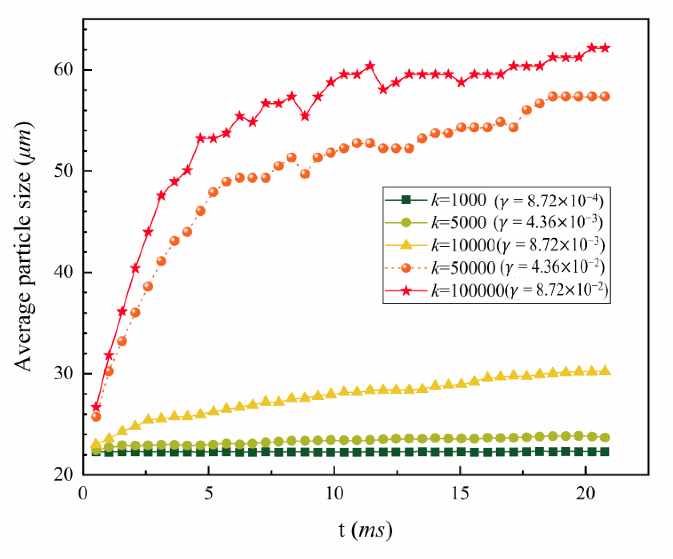
A different k in Equation (8) resulted in a different surface energy. Figure 2 shows the variation of the average particle size with different surface energy for the particles with diameter 20 μm.
If the viscosity coefficient of the particle surface was too small, the particles would bounce off after collisions, preventing the simulation of the aerosol droplet agglomeration; meanwhile, if it was too large, an abnormal contact force may appear and the calculation may be unstable. It can be seen from Figure 2 that the bonding tendency of the particles with γ = 4.36 × 10⁻² J/m2 was basically the same as that with γ = 8.72 × 10⁻² J/m2, and the average particle size was γ = 4.36 × 10⁻² J/m2. The operation was more stable and less particle separations occurred, so the surface energy value was set to 4.36 × 10⁻² J/m2 in the simulation. In addition, while increasing the surface energy, in order to ensure the stability of the calculation, it was necessary to reduce the calculation time step.
3.2. Calibration of Fluid Grid
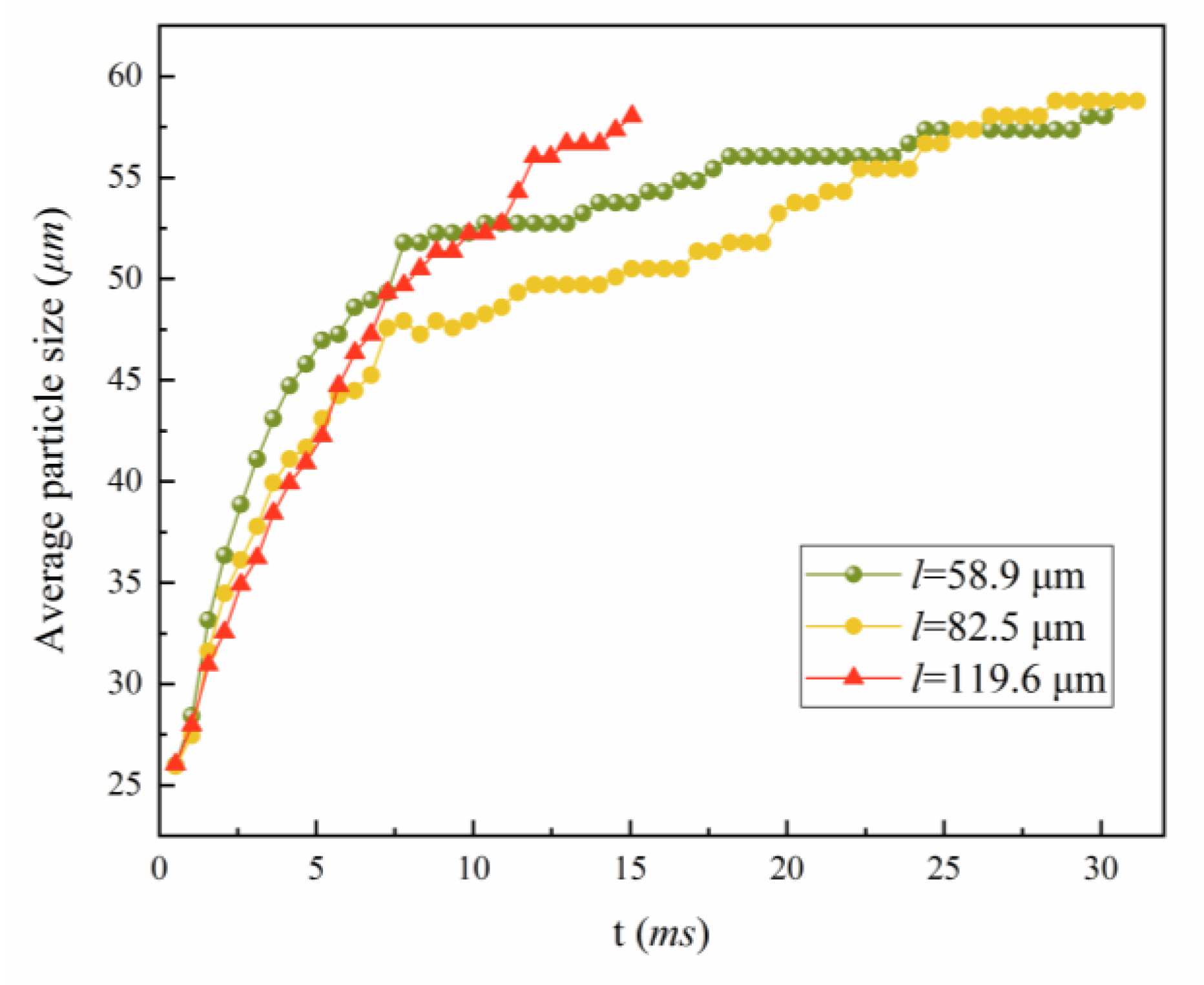
For a simulation of two-phase flow, the width of the fluid mesh was usually 3–5 times that of the average particle size [28]. The simulation took the diameter of the median particle 20 μm as the average diameter, and thus, the fluid grid of 59.8 μm (about three times of the average particle diameter), 82.5 μm (about four times of the average particle diameter), and 119.6 μm (about five times) were used for calibration. With other consistent parameters, the calculated average particle sizes are shown in Figure 3.
When the fluid grid width is 119.6 μm, the simulation terminated prematurely owing to calculation errors. Compared with the simulations with fluid grid widths of 59.8 μm and 82.5 μm, the simulated results before 25 ms varied, but the difference in the average particle size after 25 ms was small. As this study focused on the later output, the gap between simulations using 59.8 μm and 82.5 μm fluid grid was not large. Considering the simulation accuracy and calculation time simultaneously, in this study, the fluid grid with a width of 82.5 μm (four times that of the particle size) was selected in this study.
3.3. Calibration of the Time Fraction
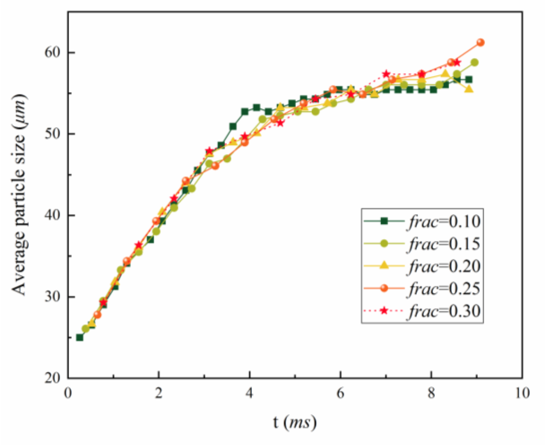
In the simulation, the critical time step was calculated based on the propagation velocity of the Rayleigh wave, which was the minimum time required by the wave to pass through each particle. To ensure the stability of the calculation, a fraction was needed on the basis of the critical time step, called the time fraction (frac). With a value of frac that was too large, the calculation was unstable, while for a frac value that was too small, the calculation time increased. The simulation results for different time fraction parameters are shown in Figure 4.
It can be seen from Figure 4 that the simulated results with different time fraction parameters were close during the initial stage, while the calculated average particle sizes with time fraction values of 0.25 and 0.30 increased faster than that with the time fraction of 0.10, and there was the tendency for continuous growth. For visualization purposes, Table 3 shows the relative errors of the calculated average particle size with different time fraction parameters at 7.79 ms.
From Table 3, it can be seen that as the time fraction increased, the simulation error also increased. Although it appears that the relative error was not large at present, the trend lines in Figure 1 indicated that the simulation error may have continued to increase. To comprehensively understand the accuracy and efficiency of the simulation, the value of frac was set to 0.20.
4. Results
The parameters of surface energy, fluid grid size, and time fraction were calibrated above, considering the simulation accuracy and efficiency, as shown in Table 4.
The particle information output from the simulation indicated the number of both single particles and multimers, as well as the information pertaining to each particle. During the data processing, the change in the number of particles was analysed, and the average particle sizes at each instant could be calculated. Different kinds of particles could also be analysed, including single particles, a dimer composed of two particles, a trimer composed of three particles, and so on. The maximum particle number of these multimers referred to the number of particles in the multimer consisting of the most particles after an iteration. The halving time of the number of particles was defined as the average agglomeration time to quantitatively describe the speed of aerosol droplet agglomeration, which referred to the instant when the number of particles in the calculation domain was half that at the initial time. The aerosol droplet particles agglomerated faster with shorter halving time.
4.1. Equivalent Sound Waves Produced by Box Vibration
In Figure 5, two fluid grids that are far from each other are selected in the box, and are the grids of the 5th row, the 5th column, and the 20th row and the 20th column, which are represented as grid (5, 5) and grid (20, 20), respectively. The pressure changes in the two grids under different conditions were calculated, as shown in Figure 5. The results verified that the pressure of the fluid domain fluctuated during the box vibration, which was equivalent to the action of sound waves.
4.2. Acoustic Agglomeration
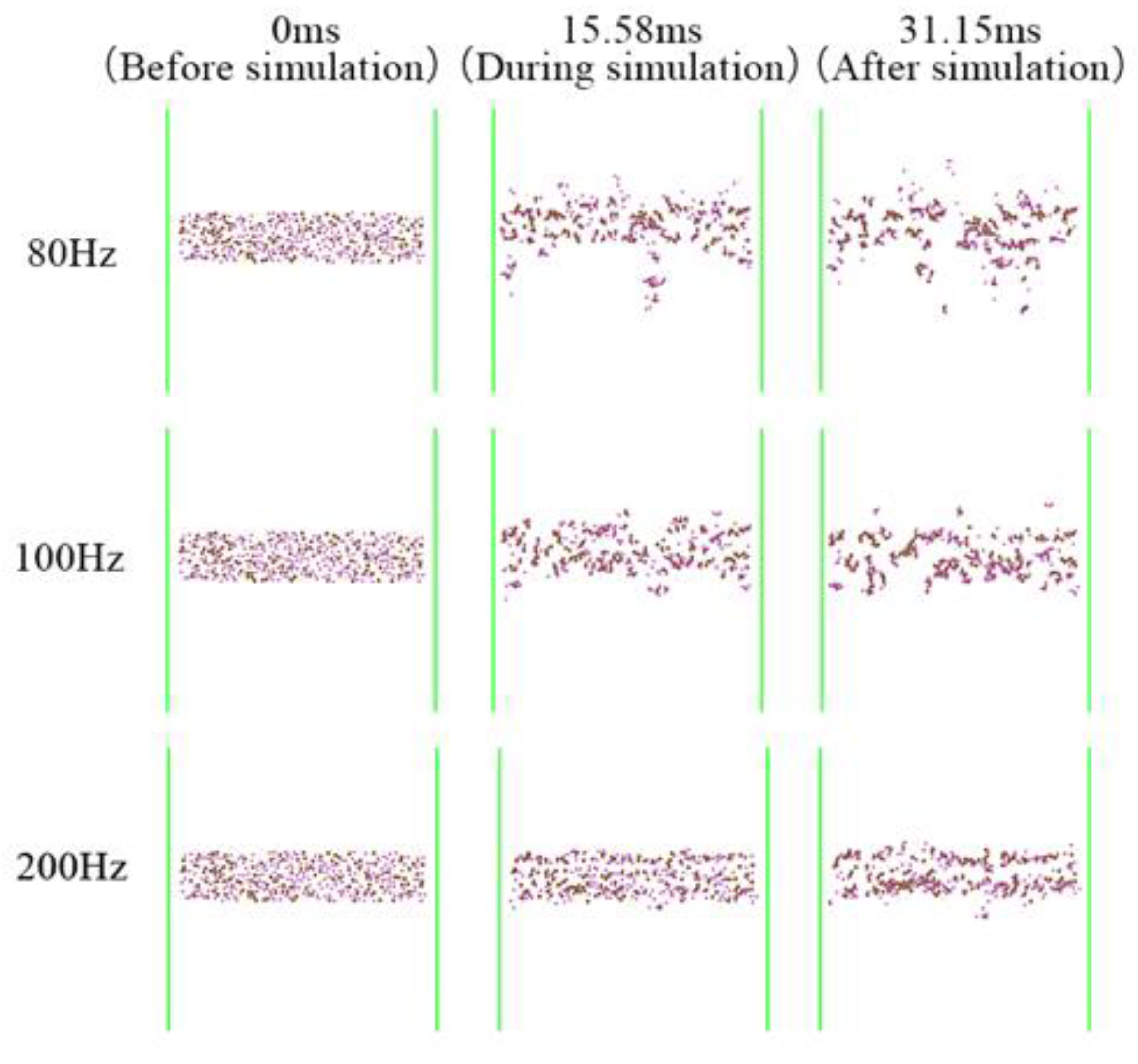
The CFD-DEM numerical model was established to simulate the agglomeration behaviour of the aerosol droplet particles under the action of sound waves. By comparing the images of the particle swarm before the simulation, during the simulation, and after the simulation, it can be clearly seen that the particles agglomerated during the simulation, and multimers were formed, as shown in Figure 6, which visually demonstrates the process of agglomeration of particles under the action of sound waves as well as the frequency effects of acoustic agglomeration.
4.3. Effect of Sound Frequency on the Agglomeration of Aerosol Droplets
In order to explore the influence of different frequencies on the motion of aerosol droplets, the SPL should be kept constant, and this was realized by adjusting the amplitude and frequency of the box vibration simultaneously. The SPL and sound frequency in the simulation were set to be 100 dB and between 60 Hz to 1000 Hz, respectively. Figure 7 shows the simulation results corresponding to different sound frequencies.
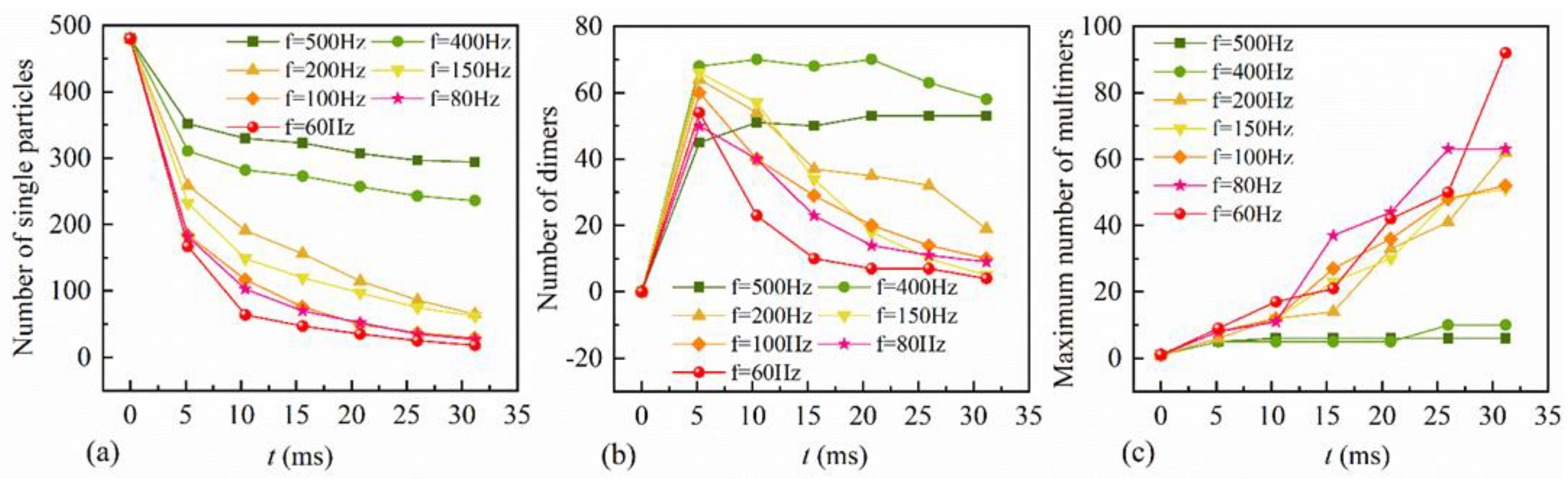
For a constant SPL, the agglomeration of aerosol droplets was affected by the sound frequency. Along with the agglomeration, the number of particles decreased and the calculated average particle size increased. Figure 7 also shows that with the decrease of frequency, the decreasing rate of the particle number became larger, and the calculated average particle size at the end of the simulation was larger, indicating that the agglomeration speed of the particles was faster under sound waves with lower frequency. Within the given frequency range, the promotion effect of the sound frequency was negatively correlated to the particle agglomeration. To further explore the agglomeration behaviour of the aerosol droplets in simulations, three parameters, i.e., the number of single particles, the number of dimers, and the maximum number of multimers, were selected for analysis, as shown in Figure 8.
Along with the simulation, the number of single particles decreased gradually under various sound frequencies. With the decrease of the sound frequency, the decreasing speed of the number of single particles increased, and the numbers decreased for all of the sound frequencies at the end of the simulation; the number of dimers first increased and then decreased, and it was larger at higher frequencies at the end of the simulation. Therefore, it was inferred that the particles do not easily collide and coagulate under higher sound frequency. At lower frequencies, the number of dimers had a maximum, and it began to decrease afterwards, owing to the participation in the coagulation of larger multimers. Generally, the probability of forming large multimers was higher with lower sound frequency. However, randomness existed in the simulation, which played an increasingly important role as the number of particles decreased. Therefore, the maximum number of multimers was not entirely negatively related to the sound frequency.
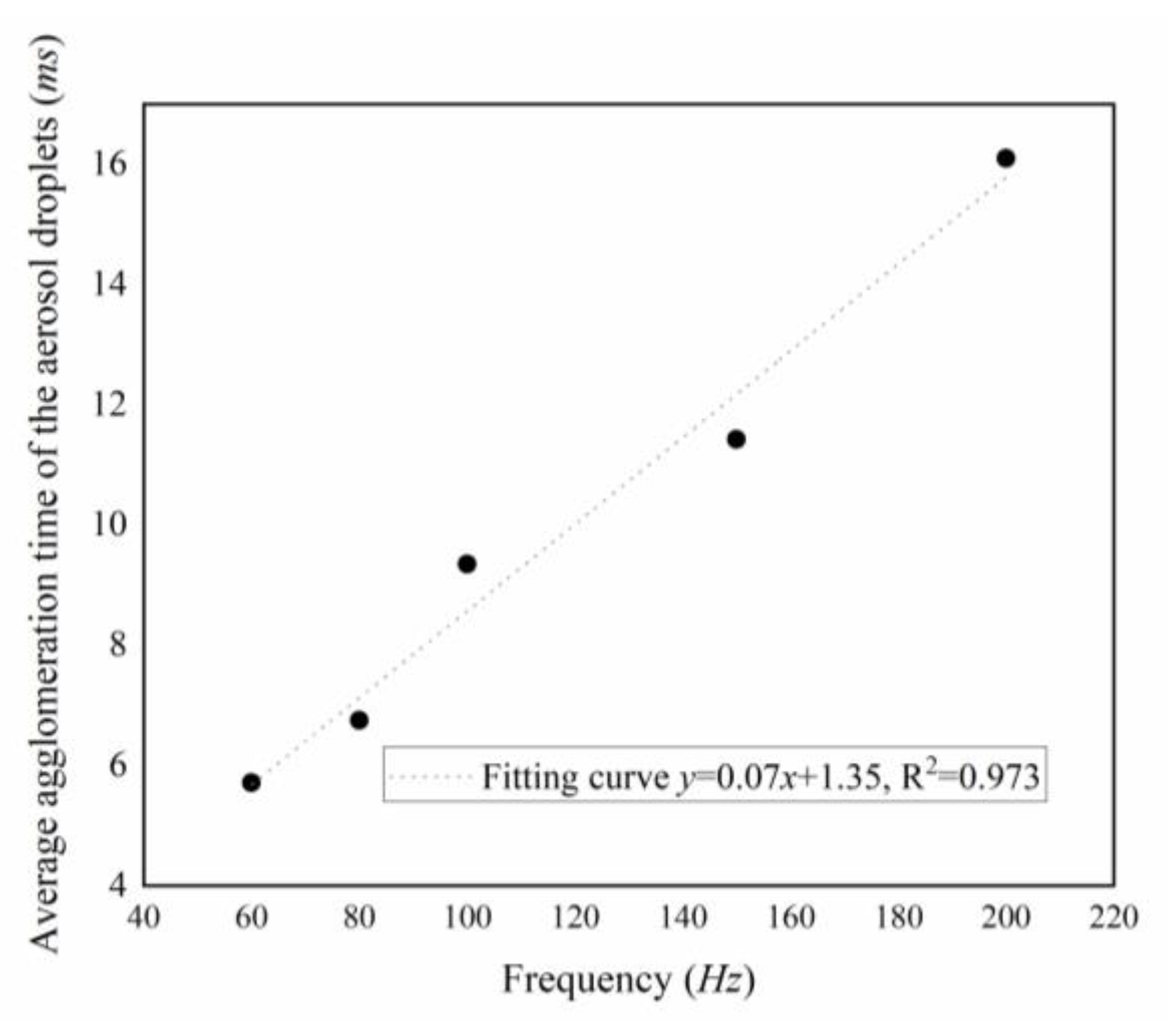
The average agglomeration time under different frequency values was studied to quantitatively describe the effect of frequency on particle agglomeration speed. As particles agglomerated quite slowly when the frequency was higher than 200 Hz, only five cases with lower frequency were analysed, as shown in Figure 9.
From Figure 9, it can be clearly seen that the agglomeration of aerosol droplets was negatively related to the sound frequency with a constant SPL for low frequencies, which can be fitted by a linear equation y = 0.07x + 1.35 with a correlation coefficient of 0.973. Thus, there existed a strong linear correlation between the average agglomeration time and the frequency of sound waves. The slope of the fitting equation was positive, indicating that the average agglomeration time increased with the increase of the sound frequency, and the agglomeration became slow. When the frequency was high (higher than 200 Hz in this simulation), the effect of sound waves on particle agglomeration was so small that the average agglomeration time was not reached during the simulation time. It can be concluded that the effect of low-frequency sound waves on aerosol droplet agglomeration was better than that of high-frequency sound waves.
4.4. Effect of SPL on the Agglomeration of Aerosol Droplets
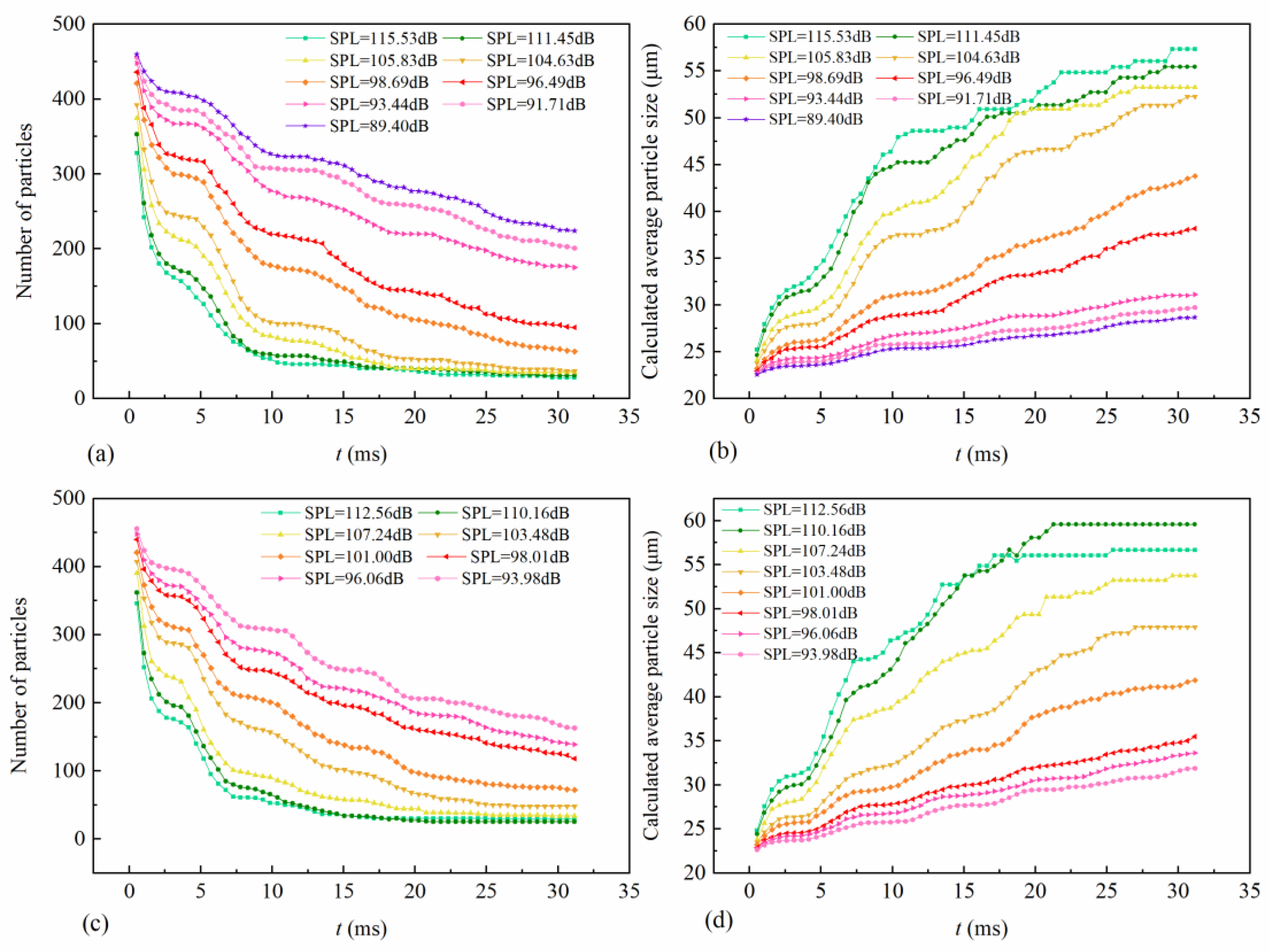
In order to explore the influence of different SPLs on the motion of aerosol droplets, the sound frequency should be kept constant. The sound wave frequency covered a wide range, and a specific frequency needed to be selected during the simulation. Previous studies proved that low frequencies had a more significant effect on particle agglomeration [29]. In this study, two low frequencies of 60 Hz and 80 Hz were selected for the simulation. Figure 10 shows the number of particles and the calculated average particle sizes during the simulation.
The influence of sound waves of 60 Hz and 80 Hz on aerosol droplet agglomeration was consistent. The number of particles decreased and the calculated average particle size increased along with the simulation. For a constant sound frequency, the speed of the particle number reduction and average particle size increase was accelerated with the increased SPL. However, when the frequency was 80 Hz, the calculated average particle size of a 112.56-dB sound wave at the end of simulation was smaller than that of the 110.16 dB sound wave. This may be due to the sharp decrease in the number of particles at the end of the simulation, and the collision was largely affected by random factors.
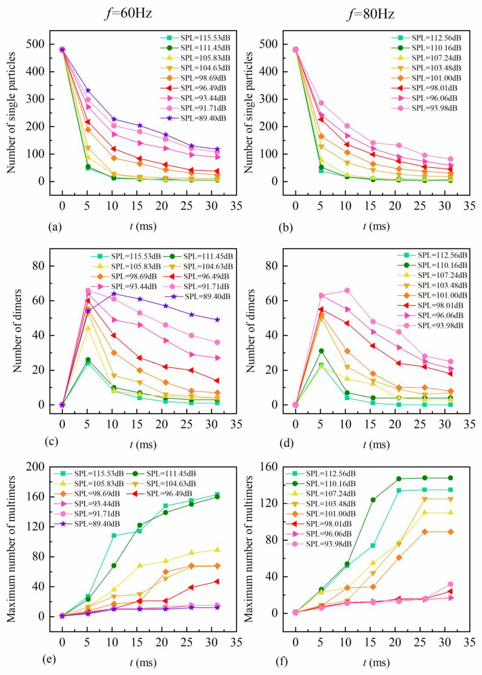
It can be seen that the SPL had a positive correlation with the promotion effect on aerosol droplet particle agglomeration, which was more obvious with larger SPL. To further explore the agglomeration of aerosol droplets during the simulation, single particles, dimers, and multimers with a maximum number of particles were selected for the analysis. A preliminary analysis found that the data output per 3000 iterations was relatively stable, and thus, the data of every 30,000 iterations was selected, i.e., one point was selected every 5.19 ms. Figure 11 shows the varying curves of the number of single particles, the number of dimers, and the maximum number of particles in the multimers.
During the simulation, the number of single particles decreased continuously, indicating that an increasing number of particles were bound to become part of the multimer under the action of sound waves. At the end of the simulation, only a few particles remained as single particles. It can be concluded that under the action of sound waves, the randomly distributed small aerosol droplet particles had a high probability of colliding, and became part of the large particles. The number of dimers increased rapidly at the beginning of the simulation, and then decreased as the simulation continued. The reason for this phenomenon is that the collision of single particles dominated the initial stage, which produced a large number of dimers. As the number of dimers increased, the probability of collision bonding between dimers and single particles, dimers, and dimers increased, and an increasing number of dimers became part of the multimers. As the number of single particles gradually decreased as the simulation progressed, the occurrence of dimers was less than the probability of collisions between single and other particles, so the number of dimers decreased. Dimers were the smallest multimers produced during the early stages of the simulation, which was the beginning and the required pathway for the formation of larger multimers. The decrease in the number of dimers was accompanied by an increase in the number of other multimers. Under the sound waves of 60 Hz and 89.4 dB, the formation of dimers was faster and their number was larger, but the rate of dimer reduction was slow, indicating that the probability of further development into multimers was greatly reduced. Thus, 89.4 dB was considered as the critical SPL of the aerosol droplets at 60 Hz, above which, chain agglomeration occurred, and vice versa. The maximum number of particles contained in the multimers gradually increased as the simulation progressed. Generally, the maximum number of particles of the multimers at the end of the simulation was higher under the sound waves with higher SPL. When the SPL increased from 89.40 dB to 93.44 dB for the 60 Hz sound waves, the maximum particle number of multimers did not change significantly, but when the SPL increased to 96.49 dB, it obviously increased. Similarly, for 80 Hz sound waves, the maximum particle number of the multimers did not change significantly when the SPL increased from 93.08 dB to 98.01 dB, while it significantly increased when the SPL increased to 101.00 dB.
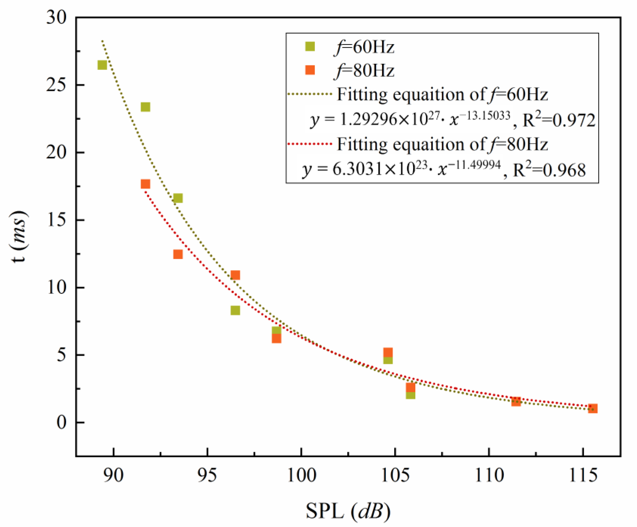
Figure 12 shows the average agglomeration time of particles under sound waves of different SPLs to quantitatively describe the effect of the SPL on the particle agglomeration speed.
The average agglomeration time was the parameter describing the agglomeration speed. With a constant frequency, the average agglomeration time was shortened with the increase of SPL, indicating faster aggregation. The curves in Figure 12 were fitted by exponential functions with good correlation. It can be inferred that when the SPL was low, corresponding to SPL values of 90~100 dB in this study, it had a greater influence on the agglomeration speed; meanwhile, when the SPL was higher, which corresponded to greater than 110 dB in this study, it had a little effect on the agglomeration speed.
By simulating 60 Hz and 80 Hz sound waves, the effects of the SPL values of sound waves on aerosol droplet agglomeration were investigated. For a constant frequency, the decreased speed of the number of multimers increased with the increase in the SPLs during the simulation. The average agglomeration time was shorter when the average particle size increased faster.
4.5. Effect of Particle Spacing on the Agglomeration of Aerosol Droplets
The number density of aerosol droplets significantly influenced the precipitation, which was generally 103/cm3 [30], i.e., the spacing between cloud droplets was about 103 μm. However, considering the computational efficiency, the calculation domain cannot be too large, so the real spacing cannot be used in simulation. The current simulation time is within milliseconds, which is far different from the fact. Therefore, the particle spacing is discussed as follows.
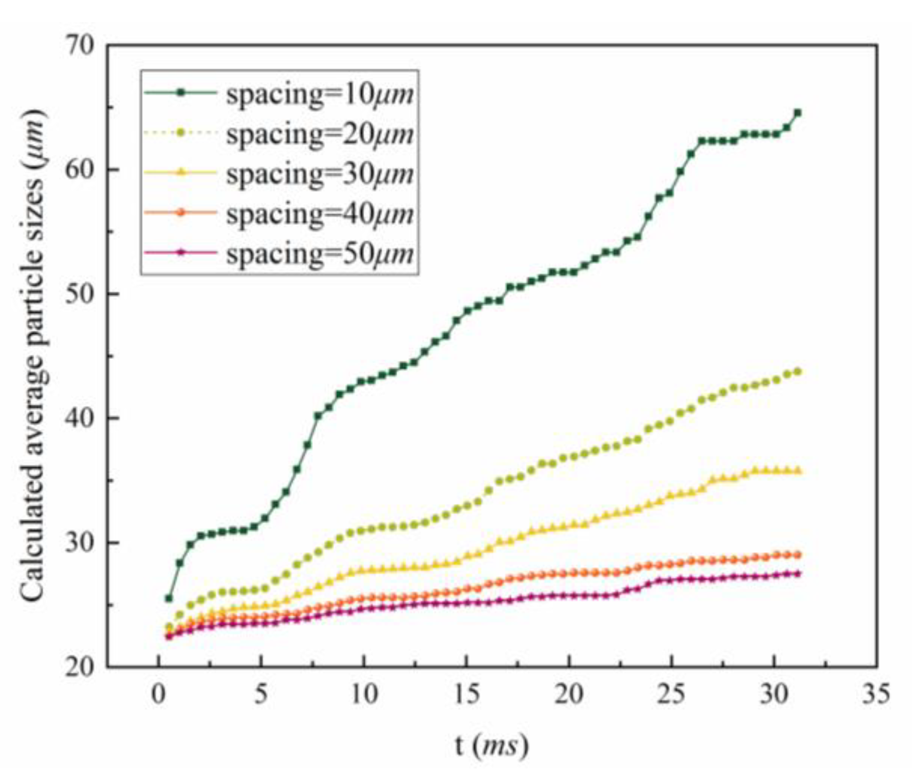
The frequency and amplitude of the box vibration remained constant in the simulation with a fixed ratio among the numbers of single particles, dimers, and multimers. Figure 13 shows the average particle sizes under different spacing conditions.
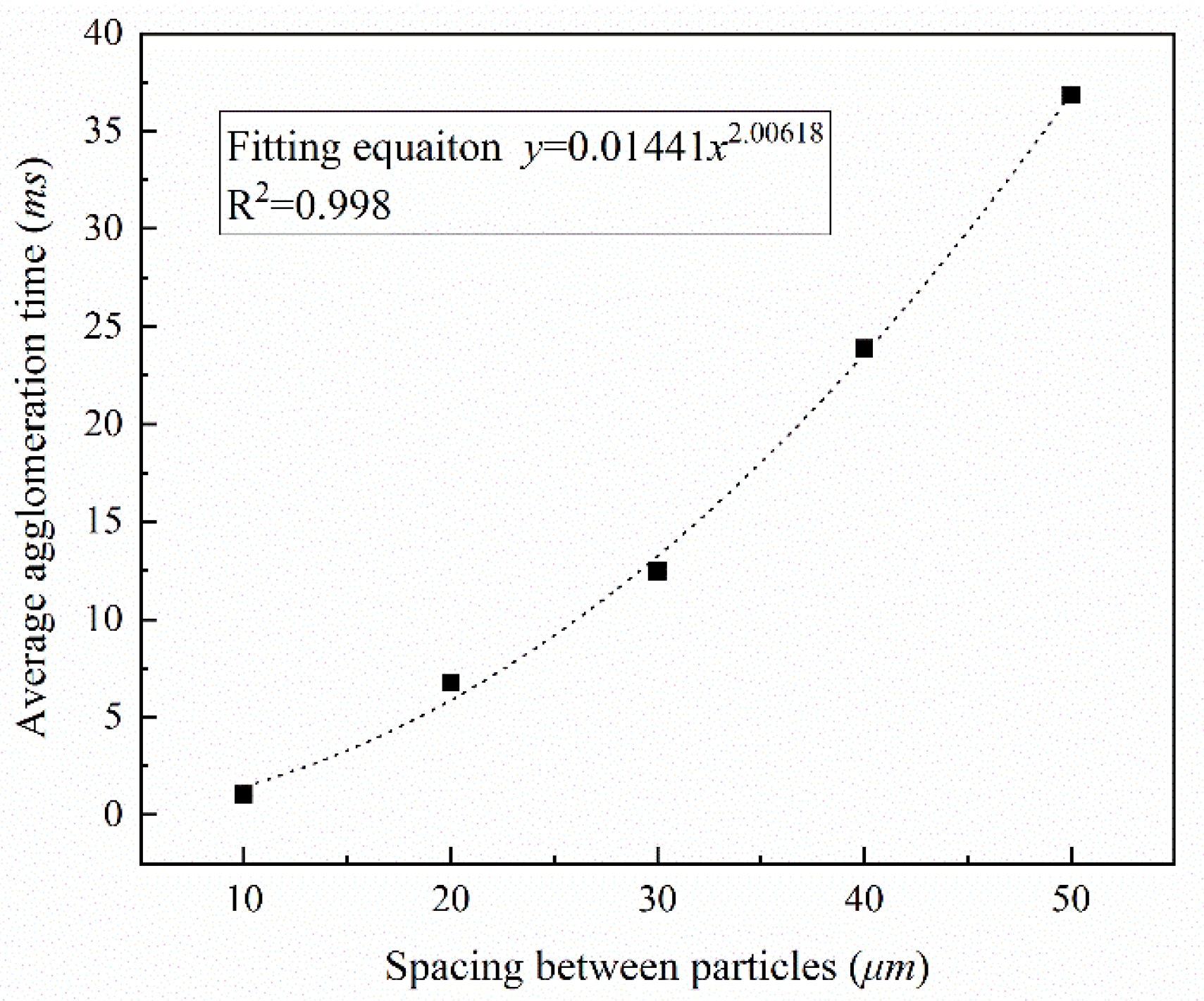
With the increased spacing, the particle agglomeration speed decreased, and the rate of growth of the calculated average particle size decreased. This is because when the spacing between the particles was large, a larger displacement was required for collision and cohesion, and it took a longer time under the same flow field. Figure 14 shows the variation of the average agglomeration time with particle spacing to better compare the effect of particle spacing on aerosol droplet agglomeration intuitively, which can be fitted by a power function with good correlation.
The average agglomeration time increased as the aerosol droplet particle spacing increased. When the particle spacing was increased to 50 μm, the average agglomeration time was about 5.5 times the value observed for the case with a droplet spacing of 20 μm. It can be inferred that under actual conditions, the average agglomeration time will increase greatly.
5. Discussion
From the simulations, it was found that the low-frequency sound waves promoted the particle agglomeration better than the high-frequency sound waves. The explanation is that the action of sound waves produced an oscillating flow field acting on the particles, and it took a period for the particles to change their motion velocity owing to the inertia. For high-frequency sound waves, the generated flow field changed rapidly; the aerosol droplet particles, especially the large ones, could not respond to the change of the oscillating flow field sufficiently fast, and the effect on the particles may have offset each other when the direction of the flow field changed, so that the effect of the sound waves on the particles was weakened. Therefore, the effect of high-frequency sound waves on aerosol droplet agglomeration was not as good as that of low-frequency sound waves. Such a conclusion was consistent with the law described in the study by Sujith [31]. However, Wang’s research suggested that there exists an optimal frequency of acoustic agglomeration resulting in the highest agglomeration efficiency [32]. This study failed to determine such an optimal frequency for aerosol droplet agglomeration, and the reason may be that the frequency range set in the simulation was not wide enough to cover the optimal value.
In addition, the sound waves with high SPL promoted particle agglomeration better than those with low SPL. This was because the SPL reflected the energy of the sound wave, and the sound waves with a high SPL contained more energy, resulting in a large amplitude of the particle movement [29]. In a two-phase flow system, there was an energy exchange, and particles under higher SPL obtained more energy. Most of this energy was converted into kinetic energy, so the movement of particles with high SPL was more intense, and there existed a greater probability of collision.
In the analysis of the effect of SPL on particle agglomeration under low-frequency sound waves, it was found that there existed a large slope in the relationship between the average agglomeration time and the SPL, and the maximum particle number of the multimers increased rapidly between the two SPLs. Therefore, for the aerosol droplet system, it was inferred that there may be a critical SPL above which the acoustic agglomeration rapidly progressed in a chain, and vice versa.
Owing to the small density of aerosol droplets under actual conditions, it was not possible to simulate the actual spacing directly in the simulation. The simulated spacing was relatively small, so the simulation time was short, i.e., of the order of milliseconds. The actual average spacing of aerosol droplets was about several dozen times that in the simulation, so the influence of the particle spacing on aerosol droplet agglomeration was explored in this study. As the particle spacing increased, the agglomeration rate slowed down, and the average agglomeration time increased. Therefore, the time scale of the aerosol droplet agglomeration under actual conditions was greater than that in simulations.
Compared with Shi et al.’s study [23], which set the mesh size of the fluid to be 3.4 mm, i.e., 340 times of the particle size (10 μm) they studied, the mesh size of fluid determined by strict sensitivity analysis in this study was only 4 times of the particle size, which better balanced the computational efficiency and accuracy. In addition, the particle size had a certain distribution instead of a unique size in this study.
Studies showed that aerosol droplet particles will continue to grow without turbulence when the size reaches about 20 μm [33]. The model in this study can be used to study the effect of different particle size distributions on the agglomeration of aerosol droplets in the future, and the generation domain can be appropriately increased, as well as the number of particles, to reduce the randomness of the result.
6. Conclusions
In this study, the agglomeration of aerosol droplets under action of sound waves was numerically studied based on the CFD-DEM calculation framework using the vibration box model. The actual physical problem was first abstracted, and then the particle model was simplified according to the research purposes. The vibration of the box was used to simulate the sound effect to establish a mechanical model. Three parameters, namely, the surface energy, fluid grid size, and time fraction value were calibrated in the parameter setting.
The simulation results verified that the relative movement of aerosol droplets was intensified under the action of strong sound waves, which promoted the occurrence of aerosol droplet agglomeration. This result confirmed the phenomenon of acoustic agglomeration proposed by Sujith et al. [31].
For sound waves with constant SPL, the low-frequency sound wave was found to have a significant effect on the agglomeration of aerosol droplets, which became more and more obvious with the increase of the SPLs. The low-frequency sound waves were also found to be more helpful in the formation of larger multimers, which was consistent with the agglomeration law of fine particles under the action of sound waves reported by Wang [32]. The correlation between the average agglomeration time and frequency showed that they are positively correlated, i.e., low-frequency sound waves promoted the aerosol droplet agglomeration better than high-frequency sound waves. For a constant frequency, the sound wave promotion effect was enhanced as the SPL increased, and the average agglomeration time and the SPL of the sound wave exhibited a negative correlation.
The initial particle spacing also impacted the simulation results. It was found that the increased speed of the calculated average particle size decreased rapidly as the particle spacing increased, and the average agglomeration time increased significantly.
Author Contributions
Conceptualization, F.L. and J.Q.; methodology, Y.G.; software, Y.G. and H.C.; validation, H.C. and Y.J.; formal analysis, F.L., H.C. and J.Q.; investigation, H.C. and J.Q.; resources, J.Q.; data curation, H.C.; writing—original draft preparation, F.L. and H.C.; writing—review and editing, F.L. and J.Q.; visualization, H.C.; supervision, J.Q.; project administration, J.Q.; funding acquisition, F.L. and J.Q. All authors have read and agreed to the published version of the manuscript.
Funding
This research was funded by the National Natural Science Foundation of China, grant numbers 91847302, 51879137, and 51979276, the Key R&D program of Science and Technology Department of Tibet under Grant No. XZ202101ZY0003G, the Joint Open Research Fund Program of State key Laboratory of Hydroscience and Engineering and Tsinghua – Ningxia Yinchuan Joint Institute of Internet of Waters on Digital Water Governance (No. sklhse-2021-Iow05), the “Smart Eye Action” under Grant No. WB2022-012, and the Youth Project of the Natural Science Foundation of Qinghai Province in China under Grants No. 2021-ZJ-934Q.
Data Availability Statement
The data presented in this study are available upon request from the corresponding author.
Conflicts of Interest
The authors declare no conflict of interest.
References
- Hoffmann, T.L.; Chen, W.; Koopmann, G.H.; Scaroni, A.W.; Song, L. Experimental and Numerical Analysis of Bimodal Acoustic Agglomeration. J. Vib. Acoust. 1993, 115, 232–240. [Google Scholar] [CrossRef]
- Tiwary, R.; Reethof, G.; Mcdaniel, O.H. Acoustically Generated Turbulence and Its Effect on Acoustic Agglomeration. J. Acoust. Soc. Am. 1984, 76, 841–849. [Google Scholar] [CrossRef]
- Patterson, H.S.; Cawood, W. Cawood, Phenomena in a sounding tube. Nature 1931, 127, 667. [Google Scholar] [CrossRef]
- Gallego-Juárez, J.A.; De Sarabia, E.R.-F.; Rodríguez-Corral, G.; Hoffmann, T.L.; Gálvez-Moraleda, J.C.; Rodríguez-Maroto, J.J.; Gómez-Moreno, F.J.; Bahillo-Ruiz, A.; Martín-Espigares, M.; Acha, M. Application of acoustic agglomeration to reduce fine particle emissions from coal combustion plants. Environ. Sci. Technol. 1999, 33, 3843–3849. [Google Scholar] [CrossRef] [Green Version]
- Fan, F.X.; Zhang, M.J.; Kim, C.N. Numerical simulation of interaction between two PM2.5 particles under acoustic travelling wave conditions. AIP Conf. Proc. 2013, 1542, 855–858. [Google Scholar]
- Wei, J.; Qiu, J.; Li, T.; Huang, Y.; Qiao, Z.; Cao, J.; Zhong, D.; Wang, G. Cloud and precipitation interference by strong low-frequency sound wave. Sci. China Technol. Sci. 2020, 64, 261–272. [Google Scholar] [CrossRef]
- Mednikov, E.P. Acoustic Coagulation and Precipitation of Aerosols; Consultants Bureau: New York, NY, USA, 1965. [Google Scholar]
- Maknickas, A.; Markauskas, D.; Kacianauskas, R. Discrete element simulating the hydrodynamic effects in acoustic agglomeration of micron-sized particles. Part. Sci. Technol. 2016, 34, 453–460. [Google Scholar] [CrossRef]
- Aktas, M.K.; Farouk, B. Numerical simulation of acoustic streaming generated by finite-amplitude resonant oscillations in an enclosure. J. Acoust. Soc. Am. 2004, 116, 2822–2831. [Google Scholar] [CrossRef]
- Otto, E.; Fissan, H. Brownian coagulation of submicron particles. Adv. Powder Technol. 1999, 10, 1–20. [Google Scholar] [CrossRef]
- Zhang, G.; Liu, J.; Wang, J.; Zhou, J.; Cen, K. Numerical simulation of acoustic wake effect in acoustic agglomeration under Oseen flow condition. Chin. Sci. Bull. 2012, 57, 2404–2412. [Google Scholar] [CrossRef] [Green Version]
- Knoop, C.; Fritsching, U. Dynamic forces on agglomerated particles caused by high-intensity ultrasound. Ultrasonics 2014, 54, 763–769. [Google Scholar] [CrossRef] [PubMed]
- Sepehrirahnama, S.; Lim, K.-M.; Chau, F.S. Numerical Analysis of the Acoustic Radiation Force and Acoustic Streaming Around a Sphere in an Acoustic Standing Wave. Phys. Procedia 2015, 70, 80–84. [Google Scholar] [CrossRef] [Green Version]
- Li, F.-F.; Jia, Y.-H.; Wang, G.-Q.; Qiu, J. Mechanism of Cloud Droplet Motion under Sound Wave Actions. J. Atmos. Ocean. Technol. 2020, 37, 1539–1550. [Google Scholar] [CrossRef]
- Jia, Y.-H.; Li, F.-F.; Fang, K.; Wang, G.-Q.; Qiu, J. Interaction between Strong Sound Waves and Cloud Droplets: Theoretical Analysis. J. Appl. Meteorol. Climatol. 2021, 60, 1373–1386. [Google Scholar] [CrossRef]
- Zhou, D.; Luo, Z.; Jiang, J.; Chen, H.; Lu, M.; Fang, M. Experimental study on improving the efficiency of dust removers by using acoustic agglomeration as pretreatment. Powder Technol. 2016, 289, 52–59. [Google Scholar] [CrossRef]
- Amiri, M.; Sadighzadeh, A.; Falamaki, C. Experimental Parametric Study of Frequency and Sound Pressure Level on the Acoustic Coagulation and Precipitation of PM2.5 Aerosols. Aerosol Air Qual. Res. 2016, 16, 3012–3025. [Google Scholar] [CrossRef] [Green Version]
- Sadighzadeh, A.; Mohammadpour, H.; Omidi, L.; Jafari, M.J. Application of acoustic agglomeration for removing sulfuric acid mist from air stream. Sustain. Environ. Res. 2018, 28, 20–24. [Google Scholar] [CrossRef]
- Cao, H.; Li, F.-F.; Zhao, X.; Liu, Z.-L.; Wang, G.-Q.; Qiu, J. Micro-droplet deposition and growth on a glass slide driven by acoustic agglomeration. Exp. Fluids 2021, 62, 127. [Google Scholar] [CrossRef]
- Qiu, J.; Tang, L.-J.; Cheng, L.; Wang, G.-Q.; Li, F.-F. Interaction between strong sound waves and cloud droplets: Cloud chamber experiment. Appl. Acoust. 2021, 176, 107891. [Google Scholar] [CrossRef]
- Markauskas, D.; Kačianauskas, R.; Maknickas, A. Numerical particle-based analysis of the effects responsible for acoustic particle agglomeration. Adv. Powder Technol. 2015, 26, 698–704. [Google Scholar] [CrossRef]
- Kacianauskas, R.; Maknickas, A.; Vainorius, D. DEM analysis of acoustic wake agglomeration for mono-sized microparticles in the presence of gravitational effects. Granul. Matter 2017, 19, 48. [Google Scholar] [CrossRef]
- Shi, Y.; Wei, J.; Qiu, J.; Chu, H.; Bai, W.; Wang, G. Numerical study of acoustic agglomeration process of droplet aerosol using a three-dimensional CFD-DEM coupled model. Powder Technol. 2019, 362, 37–53. [Google Scholar] [CrossRef]
- Sujith, R.I.; Waldherr, G.A.; Jagoda, J.I.; Zinn, B.T. A Theoretical Investigation of the Behavior of Droplets in Axial Acoustic Fields. J. Vib. Acoust. 1999, 121, 286–294. [Google Scholar] [CrossRef]
- Behbahani, M.; Behr, M.; Hormes, M.; Steinseifer, U.; Arora, D.; Coronado, O.; Pasquali, M. A review of computational fluid dynamics analysis of blood pumps. Eur. J. Appl. Math. 2009, 20, 363–397. [Google Scholar] [CrossRef] [Green Version]
- Di Felice, R. The voidage function for fluid-particle interaction systems. Int. J. Multiph. Flow 1994, 20, 153–159. [Google Scholar] [CrossRef]
- Johnson, K.L.; Kendall, K.; Roberts, A.D.; Tabor, D. Surface energy and the contact of elastic solids. Proc. R. Soc. Lond. A Math. Phys. Sci. 1971, 324, 301–313. [Google Scholar]
- Guo, Y. A Coupled DEM/CFD Analysis of Die Filling Process. Ph.D. Thesis, University of Birmingham, Birmingham, UK, 2010. [Google Scholar]
- Li, Q. Experiments and Numerical Simulation of the PM2.5 Particle Coagulation in Acoustic Field. Master’s Thesis, North China Electric Power University, Beijing, China, 2007. (In Chinese). [Google Scholar]
- Hoffmann, T.L. Environmental implications of acoustic aerosol agglomeration. Ultrasonics 2000, 38, 353–357. [Google Scholar] [CrossRef]
- Sujith, R.I. Behavior of Droplets in Axial Acoustic Fields. Ph.D. Thesis, Georgia Institute of Technology, Atlanta, GA, USA, 1994. [Google Scholar]
- Wang, J. Study of Combined Acoustic Agglomeration with Other Means to Remove Coal-Fired Fine Particles. Ph.D. Thesis, Zhejiang University, Zhejiang, China, 2012. [Google Scholar]
- East, T.W.R.; Marshall, J.S. Turbulence in Clouds as a Factor in Precipitation. Q. J. R. Meteorol. Soc. 1954, 80, 26–47. [Google Scholar] [CrossRef] [Green Version]
Figure 1.
Model schematic: (a) overall schematic; (b) partial enlarged detail of the generation domain.
Figure 1.
Model schematic: (a) overall schematic; (b) partial enlarged detail of the generation domain.

Figure 2.
Variation of the average particle size with different surface energy values for the 20 μm particles.
Figure 2.
Variation of the average particle size with different surface energy values for the 20 μm particles.

Figure 3.
Calculated average particle sizes with different fluid grids, where l is the width of the fluid grid.
Figure 3.
Calculated average particle sizes with different fluid grids, where l is the width of the fluid grid.

Figure 4.
Calculated average particle sizes with different time fraction parameters.

Figure 5.
Variation in the fluid pressure in grid (5, 5) and grid (20, 20) with the vibration frequency of 80 Hz for particle size of (a) 60 μm, (b) 80 μm, (c) 100 μm, and (d) 150 μm.
Figure 5.
Variation in the fluid pressure in grid (5, 5) and grid (20, 20) with the vibration frequency of 80 Hz for particle size of (a) 60 μm, (b) 80 μm, (c) 100 μm, and (d) 150 μm.

Figure 6.
Simulation results of the acoustic agglomeration under the sound waves with SPL = 100 dB for different sound frequencies.
Figure 6.
Simulation results of the acoustic agglomeration under the sound waves with SPL = 100 dB for different sound frequencies.

Figure 7.
Simulation of acoustic agglomeration process of aerosol droplet particles under sound waves of SPL = 100 dB: (a) decreasing process of the number of particles, (b) growth process of the calculated average particle sizes.
Figure 7.
Simulation of acoustic agglomeration process of aerosol droplet particles under sound waves of SPL = 100 dB: (a) decreasing process of the number of particles, (b) growth process of the calculated average particle sizes.

Figure 8.
Evolution of (a) the number of single particles, (b) the number of dimers, and (c) the maximum number of multimers in the simulation under sound waves of SPL = 100 dB.
Figure 8.
Evolution of (a) the number of single particles, (b) the number of dimers, and (c) the maximum number of multimers in the simulation under sound waves of SPL = 100 dB.

Figure 9.
Variation in the average agglomeration time of the aerosol droplets with the change of frequencies.
Figure 9.
Variation in the average agglomeration time of the aerosol droplets with the change of frequencies.

Figure 10.
Impact of the SPLs on aerosol droplet particles’ agglomeration: (a) plots of calculated average particle size under sound waves of f = 60 Hz; (b) plots of the number of particles under sound waves of f = 60 Hz; (c) plots of calculated average particle size under sound waves of f = 80 Hz; (d) plots of the number of particles under sound waves of f = 80 Hz.

Figure 11.
Plots of (a) the number of single particles for 60 Hz sound waves, (b) the number of single particles for 80 Hz sound waves, (c) the number of dimers for 60 Hz sound waves, (d) the number of dimers for 80 Hz sound waves, (e) the maximum number of particles in the multimers for 60 Hz sound waves, and (f) the maximum number of particles in the multimers for 80 Hz sound waves.

Figure 12.
Average agglomeration time of particles under sound waves of different SPL.

Figure 13.
Variation of the average particle sizes under different spacing conditions.

Figure 14.
Variation of average agglomeration time with droplet spacing.


Table 1.
SPL under different sound frequency values for particles of different sizes.
| A (μm) | 60 | 80 | 100 | 150 | 200 | 300 | 400 | 600 | 800 |
|---|---|---|---|---|---|---|---|---|---|
| f = 60 Hz | |||||||||
| Δp (Pa) | 0.59 | 0.77 | 0.94 | 1.34 | 1.72 | 3.41 | 3.92 | 7.47 | 12.00 |
| SPL (dB) | 89.40 | 91.71 | 93.44 | 96.49 | 98.69 | 104.63 | 105.83 | 111.45 | 115.53 |
| f = 80 Hz | |||||||||
| Δp (Pa) | 1.00 | 1.27 | 1.59 | 2.25 | 2.99 | 4.61 | 6.45 | 8.45 (A = 500μm) | |
| SPL (dB) | 93.08 | 96.06 | 98.01 | 101.00 | 103.48 | 107.24 | 110.16 | 112.52 | |
Table 2.
Sound frequency and particle size corresponding to the SPL around 100 dB.
| A (μm) | 5 | 7 | 10 | 13 | 30 | 85 | 131 | 240 |
|---|---|---|---|---|---|---|---|---|
| f (Hz) | 1000 | 800 | 500 | 400 | 200 | 100 | 80 | 60 |
| Δp (Pa) | 1.915 | 1.935 | 2.075 | 2.015 | 2.135 | 2.05 | 2.035 | 1.945 |
| SPL (dB) | 99.62 | 99.71 | 100.32 | 100.06 | 100.57 | 100.21 | 100.15 | 99.76 |
Table 3.
Relative errors of the calculated average particle size with different frac values at 7.79 ms.
Table 3.
Relative errors of the calculated average particle size with different frac values at 7.79 ms.
| Frac | 0.10 | 0.15 | 0.20 | 0.25 | 0.30 |
|---|---|---|---|---|---|
| Calculated average particle size (μm) | 55.43 | 56.04 | 56.68 | 57.34 | 57.34 |
| Relative errors with frac = 0.10 | 1.10% | 2.25% | 3.45% | 3.45% |
Table 4.
Results of parameter calibration of the model.
| Parameters | Surface Energy | Fluid Grid Size | Time Fraction |
|---|---|---|---|
| Value | 4.36 × 10⁻² J/m2 | 82.5 μm | 0.20 |
Publisher’s Note: MDPI stays neutral with regard to jurisdictional claims in published maps and institutional affiliations. |
© 2022 by the authors. Licensee MDPI, Basel, Switzerland. This article is an open access article distributed under the terms and conditions of the Creative Commons Attribution (CC BY) license (https://creativecommons.org/licenses/by/4.0/).
Share and Cite
MDPI and ACS Style
Li, F.; Cao, H.; Jia, Y.; Guo, Y.; Qiu, J. Interaction between Strong Sound Waves and Aerosol Droplets: Numerical Simulation. Water 2022, 14, 1661. https://0-doi-org.brum.beds.ac.uk/10.3390/w14101661
AMA Style
Li F, Cao H, Jia Y, Guo Y, Qiu J. Interaction between Strong Sound Waves and Aerosol Droplets: Numerical Simulation. Water. 2022; 14(10):1661. https://0-doi-org.brum.beds.ac.uk/10.3390/w14101661
Chicago/Turabian StyleLi, Fangfang, Han Cao, Yinghui Jia, Yu Guo, and Jun Qiu. 2022. "Interaction between Strong Sound Waves and Aerosol Droplets: Numerical Simulation" Water 14, no. 10: 1661. https://0-doi-org.brum.beds.ac.uk/10.3390/w14101661
Note that from the first issue of 2016, this journal uses article numbers instead of page numbers. See further details here.