Biosorption Parameter Estimation with Genetic Algorithm

Abstract

In biosorption research, a fairly broad range of mathematical models are used to correlate discrete data points obtained from batch equilibrium, batch kinetic or fixed bed breakthrough experiments. Most of these models are inherently nonlinear in their parameters. Some of the models have enjoyed widespread use, largely because they can be linearized to allow the estimation of parameters by least-squares linear regression. Selecting a model for data correlation appears to be dictated by the ease with which it can be linearized and not by other more important criteria such as parameter accuracy or theoretical relevance. As a result, models that cannot be linearized have enjoyed far less recognition because it is necessary to use a search algorithm for parameter estimation. In this study a real-coded genetic algorithm is applied as the search method to estimate equilibrium isotherm and kinetic parameters for batch biosorption as well as breakthrough parameters for fixed bed biosorption. The genetic algorithm is found to be a useful optimization tool, capable of accurately finding optimal parameter estimates. Its performance is compared with that of nonlinear and linear regression methods.

1. Introduction

Biosorption employs inactivated materials of biological origin as sorbents to sequester toxic pollutants such as heavy metal ions from waste streams [1,2,3]. The biosorption process is perceived as a surface phenomenon independent of metabolism, where various physico-chemical mechanisms operate. Because there is little biological basis in the uptake process, from a practical standpoint, biosorption is no different to conventional adsorption. This allows the whole process to be analyzed in terms of mathematical models developed in the adsorption literature with very few or no modifications. It is thus not surprising that most of the models used in the biosorption field were developed by the gas adsorption community. A well-known example is the Langmuir isotherm model—originally formulated for describing the physical adsorption of gases to inorganic surfaces—which is often used to correlate biosorption equilibrium data. Additional examples include simplified mass transfer models which are used to describe the kinetics of biosorption in batch contactors and continuous flow models which are used to characterize the breakthrough behavior in fixed bed columns packed with biosorbents. Although some of these models can have mechanistic relevance under some circumstances, they are often used in an empirical way to correlate the process information represented by a body of discrete data points generated from experimentation. The efficacy of these models depends on how well their parameters can be estimated from observed data.

A cursory examination of the recent biosorption literature reveals that the more popular models tend to be those that can be linearized to allow the estimation of parameters by means of linear regression. Examples of such models include the aforementioned Langmuir isotherm equation, the Freundlich isotherm equation, the pseudo-first order and second order kinetic equations, and the Bohart-Adams or bed-depth-service-time (BDST) fixed bed equation. This ease of fitting has played a large part in making these models popular in biosorption modeling. However, the use of linearized forms of nonlinear models for the purpose of parameter estimation is undesirable for numerous reasons that have been discussed repeatedly in the literature [4]. Historically, linearization procedures were developed before the proliferation of computer resources to allow practitioners to evaluate parameters in nonlinear models by graphical plots. Given their well-publicized deficiencies, it is puzzling that these graphical methods are still a firmly entrenched part of the biosorption modeling landscape in the present research environment where virtually everyone has access to computers and software capable of analyzing nonlinear functions.

To avoid the limitations associated with linearized approaches, nonlinear regression analysis is often recommended for fitting nonlinear equations to experimental data [4]. Besides standard nonlinear regression techniques, there are several stochastic search methods in the field of natural computing that can facilitate the estimation of parameters in nonlinear models. Notable examples include particle swarm optimization and genetic algorithm (GA) optimization. Recently, particle swarm optimization has been successfully applied to estimating bioaccumulation and biosorption parameters [5,6,7]. On the other hand, although the GA approach has been shown to offer good performance in a variety of application domains, it has rarely been used in biosorption studies. Recently, Leitch et al. [8] applied the GA method to a kinetic parameter estimation problem. The GA is a well-developed and robust optimization method, and several commercial software packages as well as add-ins for Microsoft Excel are available that require minimal effort by the user. Using data taken from the literature, the potential of the GA is evaluated here on its ability to provide accurate parameter estimates for a fairly wide range of equilibrium isotherm, batch kinetic and fixed bed breakthrough models. In addition, the performance of the GA is compared with that of Gauss-Newton-Levenberg-Marquardt nonlinear regression as well as ordinary linear regression in cases where models can be linearized.

2. Parameter Estimation Methods

Under the assumption that the structure of a selected model is correct, parameter estimation (known also as model calibration) aims to find the model parameters which give the best fit to a set of experimental data. A brief account of the three parameter estimation methods considered in this study: GA optimization, nonlinear regression and linear regression, is given here.

2.1. Genetic Algorithm Optimization

The GA approach, first introduced by Holland [9] and developed further by Goldberg [10], has been successfully applied to a variety of optimization problems. It is a stochastic global optimization method based on an iterative procedure that mimics the process of biological evolution. Unlike gradient-based approaches to nonlinear parameter identification, the GA method requires no calculation of the gradient and tends to find the global optimal solution without becoming trapped at local minima.

The GA used in this study is based on a scheme with a floating-point representation [11] and operates in the following manner. The algorithm begins with a population of randomly created individuals (initial parameter estimates) and each is evaluated for its fitness in solving the given optimization task. Each iteration, called a generation, involves a competitive selection to remove poor individuals. Following selection, the genetic operators of crossover and mutation are applied to the best individuals to produce offspring. These children (new parameter estimates) then form the basis for the next generation. The entire process is reiterated until convergence within a population is achieved. The selection algorithm used is a combination of tournament selection and elitism. Tournament selection works by choosing two individuals randomly from the population and bringing the better individual forward into the next generation. In the elitism case some of the best individuals are allowed to live into the next generation without disruption from crossover or mutation.

Several tuning parameters set by the user control the GA and affect its operation. These tuning parameters include the population size, crossover probability, mutation probability, and generation number. In general, choosing these tuning parameters is problem dependent. Brief experimentation indicated that the GA program was robust to tuning parameter variations. Full details of the GA optimization method are given by Goldberg [10].

To conduct nonlinear parameter identification using the GA, optimal parameters of a particular model with respect to a given set of data were determined by minimizing the sum of the squared errors (SSE) between measured and calculated values:

$$\text{SSE}={\displaystyle \sum _{j=1}^p{\left[w_j\left(y_{pred,j}-y_{exp,j}\right)\right]}^2}$$

(1)

where SSE is the objective function to be minimized, p is the number of observations, w_j is an appropriate weighting factor for observation j, taken to equal unity in this paper, and y_pred,j, y_exp,j are the model-predicted and measured values for observation j, respectively.

2.2. Nonlinear and Linear Regressions

The nonlinear regression method used here is based on a combination of Gauss-Newton and Levenberg-Marquardt algorithms. The nonlinear least-squares procedure is an iterative method requiring an initial approximation to the parameters and providing successively better approximations. The iterative process is repeated until a termination criterion is met. Model parameters were determined by minimizing the SSE between measured and calculated values. The nonlinear regression method is very efficient and converges to the optimal solution if the initial guess for the parameters is of good quality. For models that can be linearized, parameters were determined using the standard linear regression function provided in Excel.

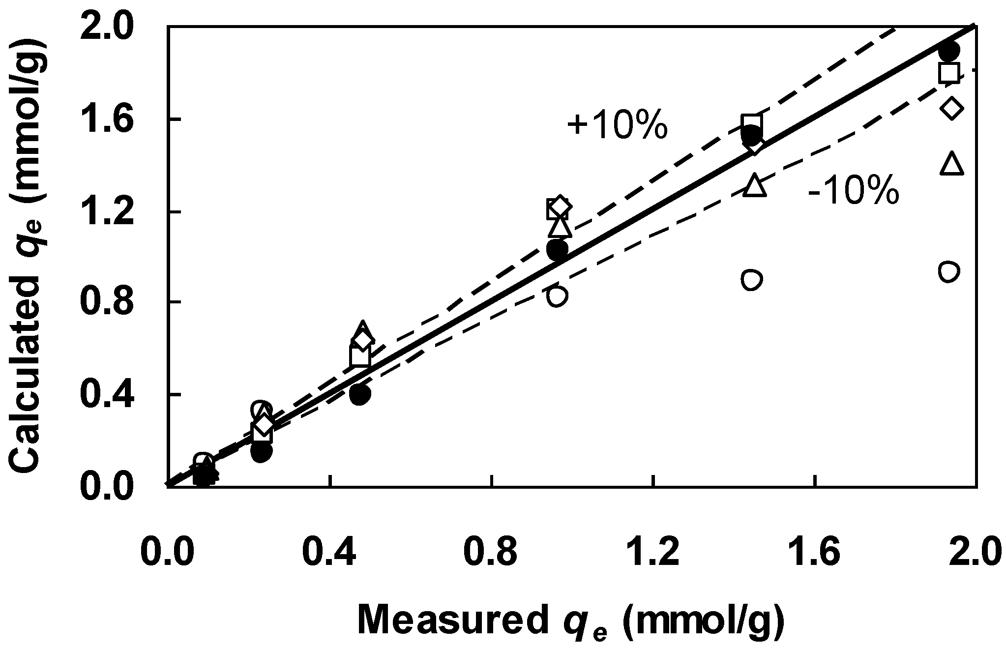
2.3. Goodness-of-Fit Measure

In this study, the following coefficient of determination (COD) is used to assess the goodness-of-fit of a model to measured data:

$$\text{COD}=\frac{{\displaystyle \sum _{j=1}^p{\left(y_{pred,j}-{\overline{y}}_{exp}\right)}^2}}{{\displaystyle \sum _{j=1}^p{\left(y_{pred,j}-{\overline{y}}_{exp}\right)}^2}+{\displaystyle \sum _{j=1}^p{\left(y_{pred,j}-y_{exp,j}\right)}^2}}$$

(2)

where ${\overline{y}}_{exp}$ is the mean of measured values and all other variables are as defined above. A COD of 1 indicates a perfect fit to the data.

3. Results and Discussion

Given a model and a set of experimental data, the objective of parameter estimation is to calibrate the model so as to reproduce the experimental results in the best possible way. The test models which were used in this study fall into three groups: equilibrium isotherm models, batch kinetic models, and continuous flow fixed bed models. The model calibration or fitting was conducted using the GA optimization method and data taken from the literature. The performance of the GA was gauged relative to Gauss-Newton-Levenberg-Marquardt nonlinear regression as well as linear regression in cases where models can be linearized.

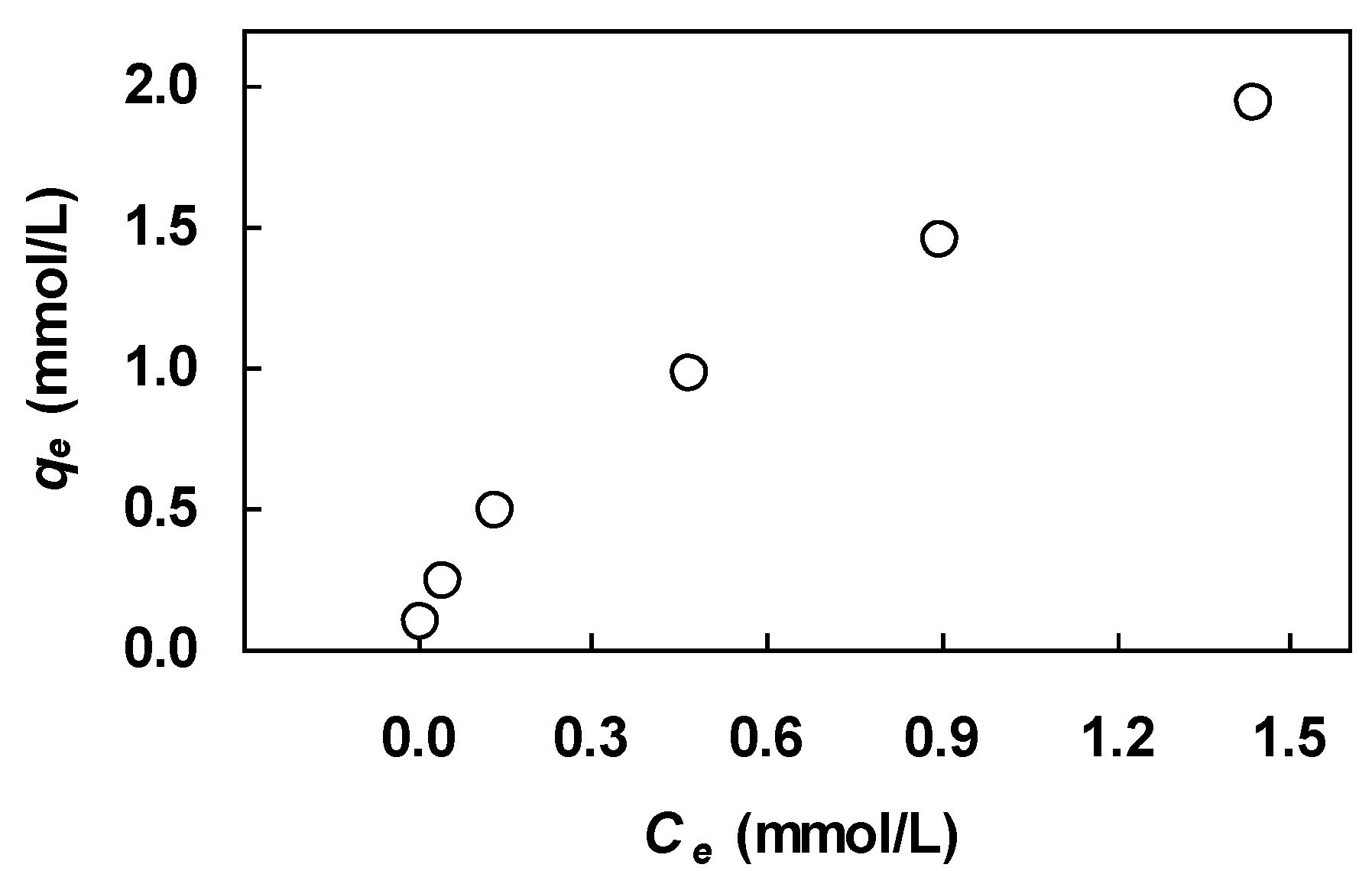
3.1. Equilibrium Isotherms

Many pure component sorption isotherms have been developed from both fundamental and empirical viewpoints. Most of these isotherms were originally developed to describe gas adsorption to porous sorbents. Here, we restrict our interest to two widely used equations: the Langmuir and the Freundlich, which have proved to be useful for engineering applications.

The two isotherm equations were fit to a set of equilibrium data on lead uptake by orange peels reported by Schiewer and Balaria [12]. This data set is interesting in that the data do not tend to a maximum asymptotically at high concentrations. It is instructive to see how well the data comply with the Langmuir and Freundlich equations. Briefly, the equilibrium experiments were conducted with a biosorbent dosage of 0.1 g/L (peel size 0.6–1 mm) in batch contactors for 3 h at pH 5 and 21–25 °C by varying the initial metal ion concentration from 20 to 400 mg/L. Samples were filtered using a 0.2-μm membrane filter, and the lead concentration of the filtrate was analyzed using atomic absorption spectrometry. The uptake on the biosorbent at equilibrium was calculated by material balance. The equilibrium data for this system are shown in Figure 1. This figure illustrates the nonlinear nature of the equilibrium relationship, which is characterized by a somewhat shallow slope at low solution concentrations and absence of a plateau at high concentrations.

Figure 1. Experimental isotherm for lead biosorption on orange peels; data of Schiewer and Balaria [12].

Figure 1. Experimental isotherm for lead biosorption on orange peels; data of Schiewer and Balaria [12].

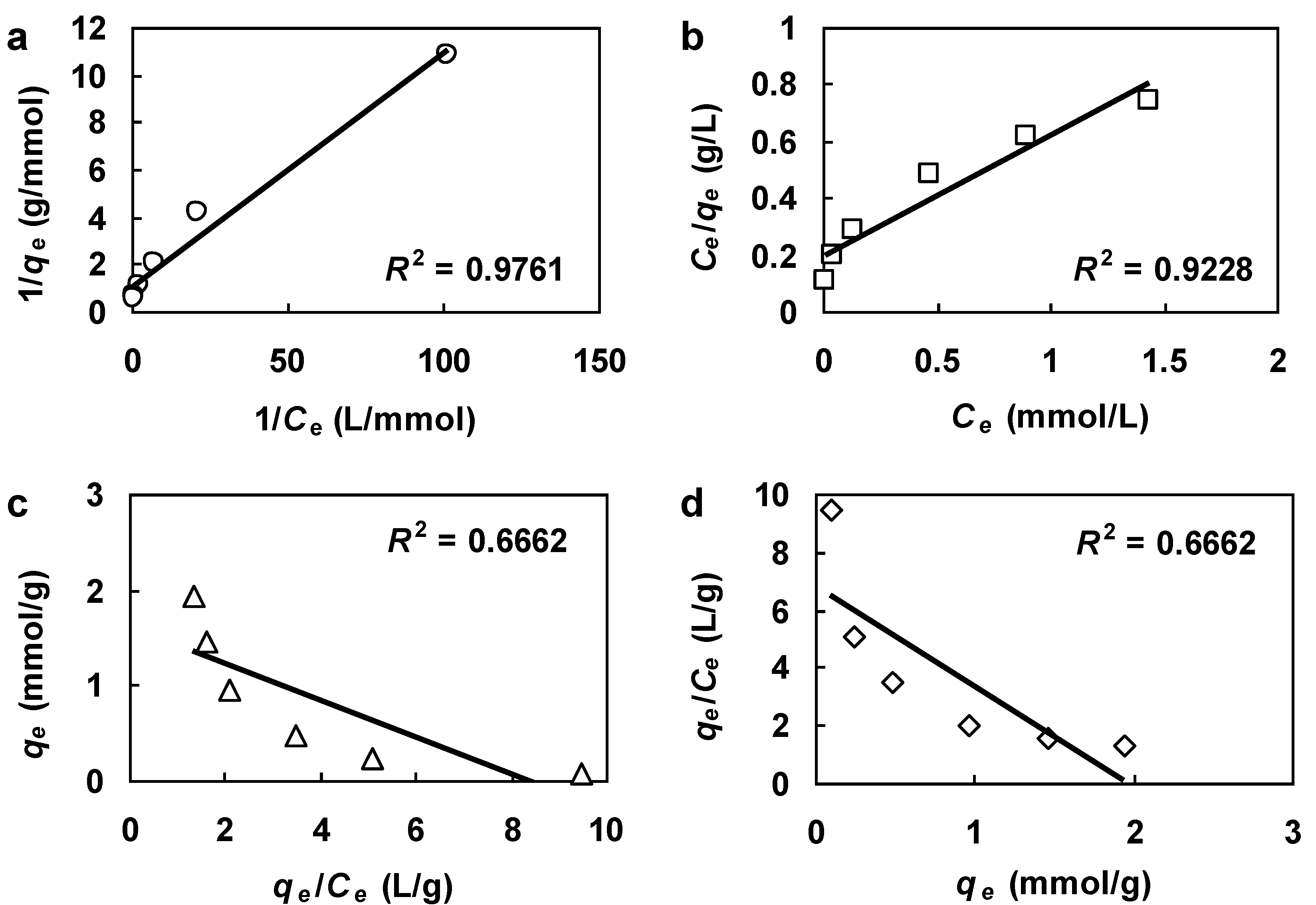
3.1.1. Langmuir equation

The two-parameter Langmuir equation is given by:

$$q_e=\frac{q_{m}b{C}_e}{1+b{C}_e}$$

(3)

where q_e is the equilibrium sorbed concentration and C_e is the equilibrium solution concentration. The two parameters to be optimized are the saturation capacity q_m and the Langmuir constant b. At sufficiently low sorbed concentrations the Langmuir equation approaches linearity (Henry’s law). At higher loadings the equation tends to a maximum asymptotically. When the product bC_e is large, Equation (3) reduces to the rectangular form typical of highly favorable sorption. The Langmuir equation is derived from a sound theoretical footing and is based on several assumptions [13]. Biosorbents, due to their complex surface structure, rarely satisfy the assumptions made in the Langmuir theory. In this context, the Langmuir equation may be viewed as a convenient tool for reproducing the correct shape of biosorption equilibrium curves rather than a mechanistic model.

The Langmuir expression has been shown to provide a useful quantitative representation of the equilibrium behavior of many biosorption systems. The standard practice in applying the Langmuir equation to biosorption data is to rearrange the equation so that q_m and b can be obtained by least-squares linear regression. Different linearization methods are available, as shown in Table 1. The terminology for the four linearized equations in Table 1 is adopted by extension from analogous linearized versions of the Michaelis-Menten equation used in enzyme kinetics studies. While linearized Michaelis-Menten equations are noted to be only of historical interest, their linearized Langmuir counterparts are still being used in the biosorption field. Plotted in Figure 2 are the linearized data of Figure 1 for the different linearization methods presented in Table 1. The goodness-of-fit indicated by R² for each plot is also given in the figure. Table 2 summarizes the values of q_m and b obtained from these transformations. COD scores calculated from Equations (2) and (3) with the derived parameters are also shown in Table 2.

Table 1. Four linearized forms of the Langmuir equation.

Linearization plot	Equation form
Lineweaver-Burk	$\frac{1}{q_e}=\frac{1}{q_{m}b}\frac{1}{C_e}+\frac{1}{q_m}\left(1/q_{e}vs1/C_e\right)$
Hanes-Woolf	$\frac{C_e}{q_e}$
Eadie-Hofstee	$q_e$
Scatchard	$\frac{q_e}{C_e}$

Table 1. Four linearized forms of the Langmuir equation.

Linearization plot	Equation form
Lineweaver-Burk	$\frac{1}{q_e}=\frac{1}{q_{m}b}\frac{1}{C_e}+\frac{1}{q_m}\left(1/q_{e}vs1/C_e\right)$
Hanes-Woolf	$\frac{C_e}{q_e}$
Eadie-Hofstee	$q_e$
Scatchard	$\frac{q_e}{C_e}$

Figure 2. Equilibrium data in Figure 1 fitted with the following linearizations: (a) Lineweaver-Burk. (b) Hanes-Woolf. (c) Eadie-Hofstee. (d) Scatchard.

Figure 2. Equilibrium data in Figure 1 fitted with the following linearizations: (a) Lineweaver-Burk. (b) Hanes-Woolf. (c) Eadie-Hofstee. (d) Scatchard.

Table 2. Parameter estimation in the Langmuir equation by the linear regression, nonlinear regression and GA methods.

Estimation method	qm (mmol/g)	b (L/mmol)	COD
Linear regression
Lineweaver-Burk	0.99	10.31	0.414
Hanes-Woolf	2.37	2.17	0.967
Eadie-Hofstee	1.60	5.20	0.809
Scatchard	1.97	3.46	0.923
Nonlinear regression	3.20	1.00	0.990
Genetic algorithm	3.20	1.00	0.990

Table 2. Parameter estimation in the Langmuir equation by the linear regression, nonlinear regression and GA methods.

Estimation method	qm (mmol/g)	b (L/mmol)	COD
Linear regression
Lineweaver-Burk	0.99	10.31	0.414
Hanes-Woolf	2.37	2.17	0.967
Eadie-Hofstee	1.60	5.20	0.809
Scatchard	1.97	3.46	0.923
Nonlinear regression	3.20	1.00	0.990
Genetic algorithm	3.20	1.00	0.990

As Figure 2 shows, the Lineweaver-Burk plot with an R² of 0.976 provided the best fit among the four linearizations. However, it also had the lowest COD (0.414), as shown in Table 2. Note that the R² value was obtained with the transformed data while the COD value was calculated on the untransformed data. It is evident that the fitted q_m and b based on the transformed data of the Lineweaver-Burk linearization perform poorly when they are substituted back into Equation (3). This phenomenon illustrates the limitations associated with the transformation of data required by the Lineweaver-Burk plot. The main problems with the Lineweaver-Burk linearization are that most of the data points clump near the origin and the slope of the linear plot is extremely sensitive to variability at low values of C_e (high values of 1/C_e) [14], as can be seen in Figure 2a. Although the Hanes-Woolf plot yielded the second highest R², it provided the best result as indicated by the highest COD score.

Next, the Langmuir equation (Equation (3)) was fit to the Figure 1 data by using the nonlinear regression and GA methods. The best parameter estimates are tabulated in Table 2. Both methods found identical parameter estimates and yielded a much higher COD score relative to the four linearizations. Of the four linearizations tested, the Hanes-Woolf plot found the most similar estimates of q_m and b to the GA. Still, the Hanes-Woolf-derived q_m and b were, respectively, 26% smaller and 117% bigger than the GA-generated q_m and b. Therefore, the GA improved the parameter accuracy considerably. Figure 3 compares the performance of the four linearizations and GA in visual terms. The Langmuir equation containing the Lineweaver-Burk-derived parameters systematically underestimated the measured values of q_e at high concentrations, suggesting that the derived parameters are not adequate at these concentration levels. All q_e values calculated with the GA-generated parameters fall close to the 1:1 line (solid line in Figure 3), confirming the superiority of the GA over the four linearizations. Although the limitations of linearized Langmuir equations have been noted for some time [14,15,16], out of inertia they are found to persist in biosorption modeling. There is little doubt that the antiquated practice of linearization has no place in today’s research environment.

Figure 3. Comparison between the Figure 1 equilibrium data and q_e calculated from the Langmuir equation (Equation (3)) containing parameters estimated from the following linearizations: Lineweaver-Burk (open circles), Hanes-Woolf (triangles), Eadie-Hofstee (diamonds), Scatchard (squares), and parameters estimated from the GA (filled circles).

Figure 3. Comparison between the Figure 1 equilibrium data and q_e calculated from the Langmuir equation (Equation (3)) containing parameters estimated from the following linearizations: Lineweaver-Burk (open circles), Hanes-Woolf (triangles), Eadie-Hofstee (diamonds), Scatchard (squares), and parameters estimated from the GA (filled circles).

3.1.2. Freundlich equation

Originally developed for gas adsorption [17], the Freundlich equation has been used extensively in the correlation of sorption of organics from aqueous solutions onto activated carbon. The two-parameter equation takes the form:

$$q_e=K_F{C}_e^{n_F}$$

(4)

where q_e, C_e are similarly defined in Equation (3) and K_F, n_F constitute the two unknown parameters. If the sorption is favorable, then n_F < 1. Unlike the Langmuir equation, Equation (4) has neither a proper Henry law behavior at low sorbed concentration nor a finite saturation limit when sorbed concentration is sufficiently high. As a result, it is not applicable over a large range of equilibrium data. The Freundlich equation may be linearized as follows:

$$\ln q_e=\ln K_F+n_F\ln C_e$$

(5)

Table 3 summarizes the optimal estimates obtained from Equation (5) by the linear regression approach and from Equation (4) by the GA and nonlinear regression methods. There was essentially no difference in the GA and nonlinear regression-derived parameters. Likewise, the differences in the parameters between the linear regression approach and the other two techniques appear trivial. In contrast to the four linearized Langmuir equations, the linearized Freundlich equation performed much better in correlating the Figure 1 data. This phenomenon is most likely due to the absence of a plateau in the data (see Figure 1).

Table 3. Parameter estimation in the Freundlich equation by the linear regression, nonlinear regression and GA methods.

Estimation method	$K_F\left(\left({\text{mmol}}^{\left(1-n_F\right)}·{\text{L}}^{n_F}\right)/\text{g}\right)$	nF	COD
Linear regression (Equation (5))	1.554	0.609	>0.999
Nonlinear regression	1.550	0.607	>0.999
Genetic algorithm	1.550	0.607	>0.999

Table 3. Parameter estimation in the Freundlich equation by the linear regression, nonlinear regression and GA methods.

Estimation method	$K_F\left(\left({\text{mmol}}^{\left(1-n_F\right)}·{\text{L}}^{n_F}\right)/\text{g}\right)$	nF	COD
Linear regression (Equation (5))	1.554	0.609	>0.999
Nonlinear regression	1.550	0.607	>0.999
Genetic algorithm	1.550	0.607	>0.999

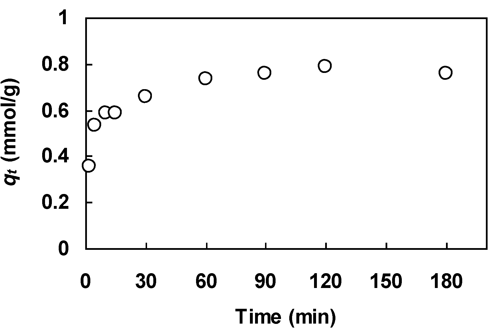
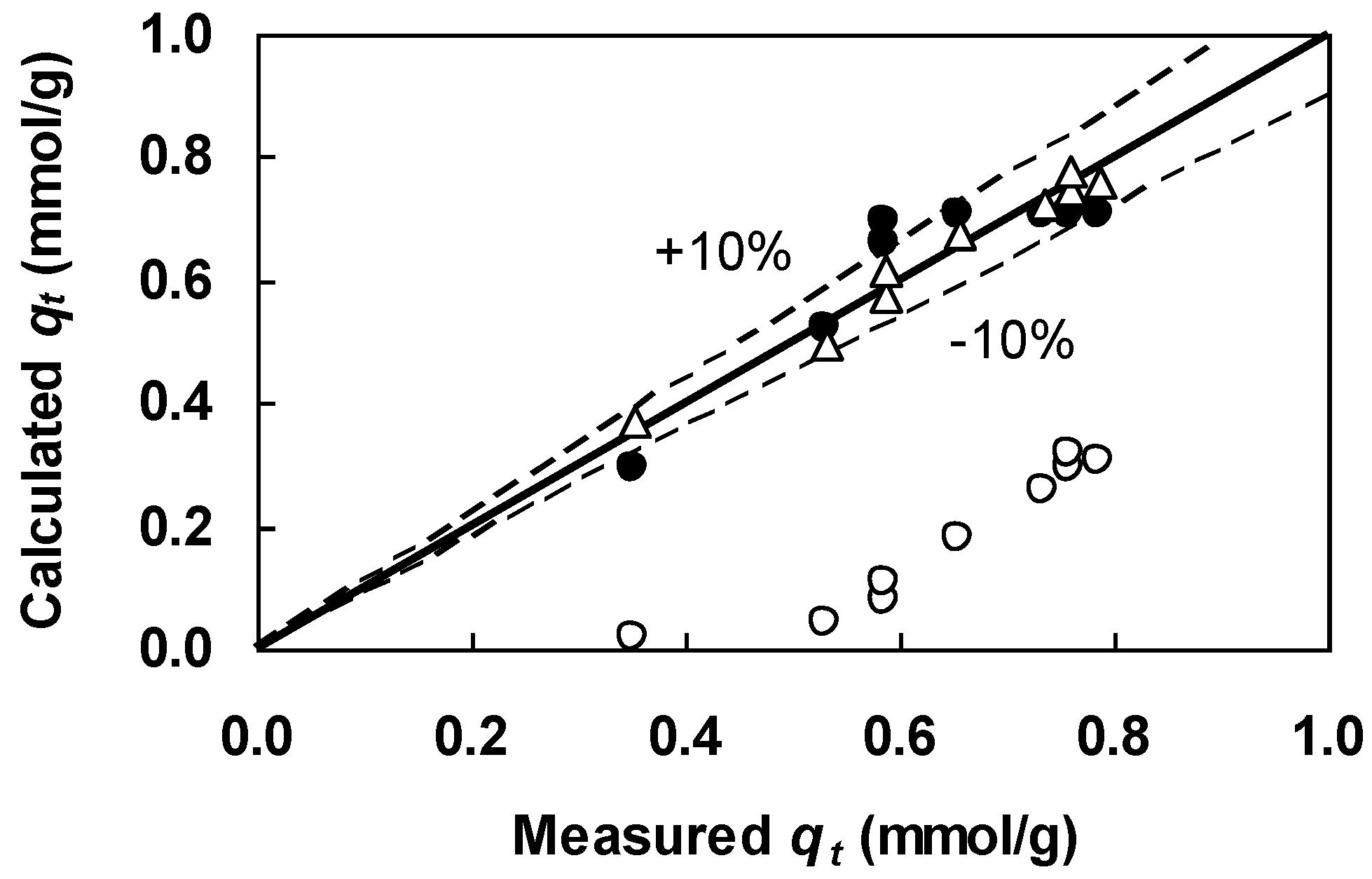
3.2. Batch Kinetic Models

Batch uptake experiments are routinely carried out to assess the kinetic behavior of pollutant sorption to the surface of a biosorbent. The time taken for the biosorbent to become saturated depends on the rate of uptake. The uptake rate could be considered reaction control if reaction is much slower than diffusion (film and/or intraparticle diffusion) or diffusion controlled if the opposite is true. The majority of biosorption studies favor the use of reaction-based kinetic models in correlating batch uptake data although no evidence is presented to indicate that diffusion is not the rate controlling mechanism for the biosorption. This is in large part due to the fact that the commonly used reaction kinetic models can be integrated to yield analytical expressions that can be linearized to allow the estimation of parameters by linear regression. Here we examine parameter estimation in one such reaction kinetic model that can be linearized, the Lagergren equation (known also as the pseudo first order rate equation), and a general nth order rate equation that cannot be linearized.

The two rate equations were fit to a set of kinetic data on lead uptake by orange peels reported by Schiewer and Balaria [12]. The kinetic experiment was conducted with an initial metal concentration of 0.1 mmol/L and a biosorbent dosage of 0.1 g/L (peel size 1–3 mm) in a batch contactor at pH 5 and 21–25 °C. Samples were taken periodically using a syringe, filtered using a 0.2-μm membrane filter, and the lead concentration of the filtrate was analyzed using atomic absorption spectrometry. The uptake on the biosorbent was calculated by material balance. Figure 4 depicts the kinetic data for this system. We chose this data set because the ascending part of the kinetic profile is well characterized by a sufficient number of data points. This is an important requirement when testing the correlative power of a kinetic model.

Figure 4. Experimental uptake curve for lead biosorption on orange peels; data of Schiewer and Balaria [12].

Figure 4. Experimental uptake curve for lead biosorption on orange peels; data of Schiewer and Balaria [12].

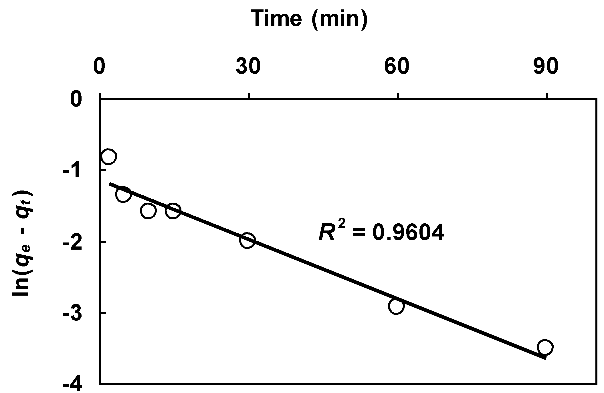
3.2.1. Lagergren equation

The century-old Lagergren rate equation [18] is given by:

$$\frac{d{q}_t}{dt}=k_1\left(q_e-q_t\right)$$

(6)

where q_t is the sorbed concentration at any time t, q_e is the equilibrium sorbed concentration, and k₁ is the first order Lagergren rate constant. The analytical solution of Equation (6) for the initial condition of q_t = 0 at t = 0 can be written as:

$$q_t=q_e\left[1-\exp \left(-k_{1}t\right)\right]$$

(7)

Equation (7) may be rearranged to yield the following linearized equation:

$$\ln \left(q_e-q_t\right)=\ln q_e-k_{1}t$$

(8)

In Equation (8) q_e and k₁ are fitting parameters. Note that this linear regression procedure requires a value of q_e in order to calculate the left side of Equation (8). The logarithmic term ln(q_e − q_t) dictates that q_e be assigned the maximum measured value. For the Figure 4 data, the maximum value is given by the second last data point measured at 120 min. The q_e term on the left side of Equation (8) was thus assigned the value of this data point (q_e = 0.79 mmol/g). Figure 5 shows the data in Figure 4 plotted according to Equation (8). It can be seen that the linear fit is satisfactory as indicated by the high value of R². The two parameters q_e and k₁ on the right side of Equation (8) were determined, respectively, from the y-intercept and slope of the linear plot. Listed in Table 4 are the derived parameters.

The fitted value of 0.32 mmol/g for q_e was much lower than the assigned value of 0.79 mmol/g for q_e which was used to generate the linear plot in Figure 5. Furthermore, the COD value was rather low (Table 4), indicating significant differences between the calculated and measured q_t. A comparison between the Figure 4 data and q_t calculated from the Lagergren equation (Equation (7)) with the derived parameters is shown in Figure 6 (open circles). The figure includes results calculated from a general nth order rate equation and these will be discussed in the next section. Figure 6 shows that all calculated values of q_t were much smaller than the measured values of q_t. The poor representation of the untransformed data indicates that the linearized Lagergren equation is inadequate for parameter estimation.

Figure 5. Kinetic data in Figure 4 plotted according to the linearized Lagergren equation (Equation (8)).

Figure 5. Kinetic data in Figure 4 plotted according to the linearized Lagergren equation (Equation (8)).

Table 4. Parameter estimation in the Lagergren equation by the linear regression, nonlinear regression and GA methods.

Estimation method	qe (mmol/g)	k1 (min−1)	COD
Linear regression (Equation (8))	0.32	0.028	0.512
Nonlinear regression	0.71	0.268	0.819
Genetic algorithm	0.71	0.268	0.819

Table 4. Parameter estimation in the Lagergren equation by the linear regression, nonlinear regression and GA methods.

Estimation method	qe (mmol/g)	k1 (min−1)	COD
Linear regression (Equation (8))	0.32	0.028	0.512
Nonlinear regression	0.71	0.268	0.819
Genetic algorithm	0.71	0.268	0.819

Tabulated in Table 4 are the best estimates obtained by fitting the Lagergren equation (Equation (7)) to the Figure 4 data using the GA and nonlinear regression methods. Both methods yielded equivalent parameter estimates. These q_e and k₁ estimates were, respectively, 122% and 857% larger than the linear regression-generated q_e and k₁. The higher COD and the proximity of calculated q_t to the 1:1 line, as indicated by the filled circles in Figure 6, suggest that the GA was capable of finding realistic parameters that fit the measured data quite well. For this data set, the performance of the linear regression approach was obviously inferior to that of the GA. Although the linearized Lagergren equation ((Equation (8)) is clearly unsatisfactory, it remains the equation of choice for parameter estimation in many biosorption studies that employ the Lagergren equation. The nonlinear Lagergren equation (Equation (7)), by contrast, is often ignored because it is necessary to go beyond linear regression in order to estimate its parameters from measured data.

Figure 6. Comparison between the Figure 4 kinetic data and q_t calculated from the Lagergren equation (Equation (7)) with the linear regression-derived parameters (open circles) and GA-generated parameters (filled circles) listed in Table 4. Also shown are q_t calculated from the nth order equation (Equation (10)) with the GA-derived parameters (triangles) given in Table 5.

Figure 6. Comparison between the Figure 4 kinetic data and q_t calculated from the Lagergren equation (Equation (7)) with the linear regression-derived parameters (open circles) and GA-generated parameters (filled circles) listed in Table 4. Also shown are q_t calculated from the nth order equation (Equation (10)) with the GA-derived parameters (triangles) given in Table 5.

3.2.2. nth Order Rate Equation

Because the integrated form of the first order Lagergren equation can be linearized, it has been used to model countless batch biosorption systems. However, as pointed out by various investigators [19,20,21,22], it makes no modeling sense to preset the reaction order which should be treated as an adjustable parameter in correlating biosorption data. Accordingly, a general nth order rate law can be written as:

$$\frac{d{q}_t}{dt}=k_n{\left(q_e-q_t\right)}^n$$

(9)

where q_t, q_e, t are similarly defined in Equation (6) and k_n, n indicate the nth order rate constant and reaction order, respectively. When n = 1 we recover the first order Lagergren equation. Note that n as defined in Equation (9) may be a noninteger. The integrated form of Equation (9) for the initial condition of q_t = 0 at t = 0 is given by [19]:

$$q_t=q_e-{\left(q_e^{\left(1-n\right)}+\left(n-1\right)k_{n}t\right)}^{1/\left(1-n\right)}$$

(10)

In Equation (10) three unknown parameters, k_n, n (n ≠ 1) and q_e, are to be determined simultaneously, which of course cannot be estimated using linear regression. Note that Equation (10) may be recovered from a more general solution of the nth order rate law incorporating the concept of fractal kinetics [23].

Equation (10) was fit to the Figure 4 data by using the GA and nonlinear regression methods, and both methods converged on the same optimal solution, as shown in Table 5. This demonstrates the efficacy of the GA as a parameter estimation tool for nonlinear models that cannot be linearized. Values of q_t calculated from Equation (10) with the GA-derived parameters are compared with the Figure 4 data in Figure 6 (triangles). Both the graphical comparison (Figure 6) and the COD statistics (Table 4 and Table 5) indicate that the three-parameter nth order rate equation provided a better description of the kinetic data compared to the two-parameter Lagergren equation. This is not surprising because models with more adjustable parameters will almost always result in a better fit. However, the fact that Equation (10) cannot be linearized is likely to limit its application in the correlation of biosorption kinetic data. Note that the nonlinear regression method was sensitive to initial parameter guesses. For instance, no convergence difficulties were observed when the starting point of the parameter vector (q_e, k_n, n) was chosen to be (10, 10, 10). However, false convergence was encountered with the starting point (100, 100, 100). As noted above, rather than operating on a single set of parameters, the GA makes use of a population of parameter sets (individuals). For the nth order rate equation, the GA was able to obtain the optimal parameter set within a search range having upper parameter limits as high as (10,000, 10,000, 10,000).

Table 5. Parameter estimation in the nth order rate equation by the nonlinear regression and GA methods.

Estimation method	qe (mmol/g)	kn ((mmol/g)1−n/min)	n	COD
Nonlinear regression	0.900.90	0.84	3.89	0.971
Genetic algorithm		0.84	3.89	0.971

Table 5. Parameter estimation in the nth order rate equation by the nonlinear regression and GA methods.

Estimation method	qe (mmol/g)	kn ((mmol/g)1−n/min)	n	COD
Nonlinear regression	0.900.90	0.84	3.89	0.971
Genetic algorithm		0.84	3.89	0.971

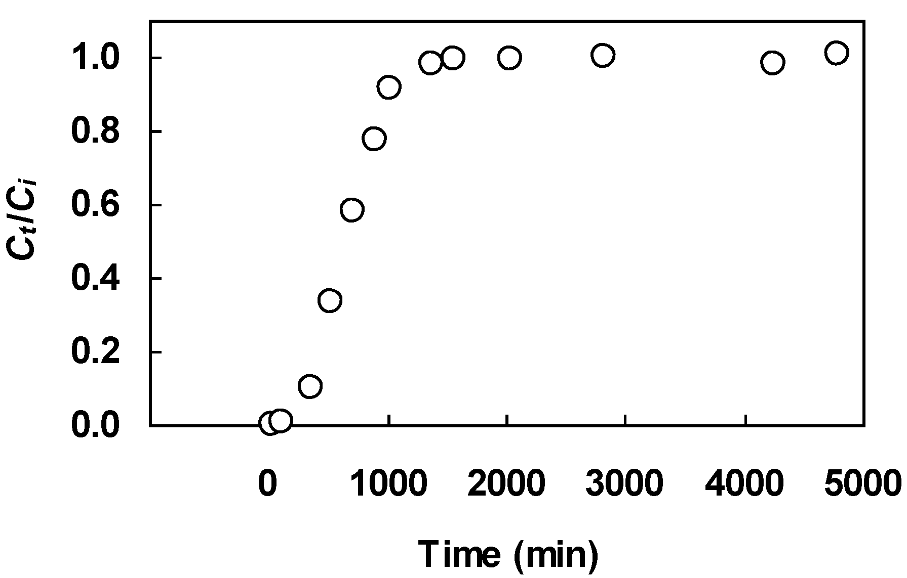
3.3. Fixed Bed Models

Commercial applications of biosorbents will most likely be conducted using fixed bed columns which are widely used in activated carbon adsorption processes. From the perspective of process modeling, the dynamic behavior of a fixed bed column is described in terms of the effluent concentration-time profile, that is, the breakthrough curve. The shape of this curve is determined by the nature of the equilibrium isotherm and influenced by the individual transport processes in the column and the sorbent.

Comprehensive fixed bed models taking account of the nonlinear equilibrium behavior and dispersive effects (axial dispersion, finite resistance to mass transfer, and sorption kinetics) are described in terms of partial differential equations and generally require a numerical solution. To circumvent the mathematical and numerical complexities, simplified or short-cut methods are used extensively for the initial design and analysis of fixed bed columns. Many of the widely used simplified models for correlating the breakthrough curves of activated carbon columns are well covered in the book by Cooney [24]. In general, these models are very straightforward, easy to apply, and provide acceptable modeling power. We illustrate here two such simplified fixed bed models that can be used to analyze biosorption columns: the Bohart-Adams equation and the Belter-Cussler-Hu equation.

The two fixed bed equations were fit to a set of breakthrough data on nickel uptake by a seaweed biosorbent reported by Borba et al. [25]. We chose this data set because all essential fixed bed details for calculating the input parameters in the Bohart-Adams equation are given in the article. The laboratory-scale column with 2.8 cm internal diameter was packed with seaweed biomass (Sargassum filipendula) to a height of 30.5 cm. The pH and temperature of the feed solution were adjusted to 3.0 and 30 °C, respectively. Several breakthrough experiments were conducted using different feed flow rates. Solution samples were taken periodically at the column outlet and analyzed for nickel concentration using atomic absorption spectrometry. One of the reported breakthrough data sets—obtained with a feed nickel concentration of 2.12 meq/L and a feed flow rate of 0.006 L/min—is shown in Figure 7.

Figure 7. Experimental breakthrough curve for nickel biosorption on seaweed biomass; data of Borba et al. [25].

Figure 7. Experimental breakthrough curve for nickel biosorption on seaweed biomass; data of Borba et al. [25].

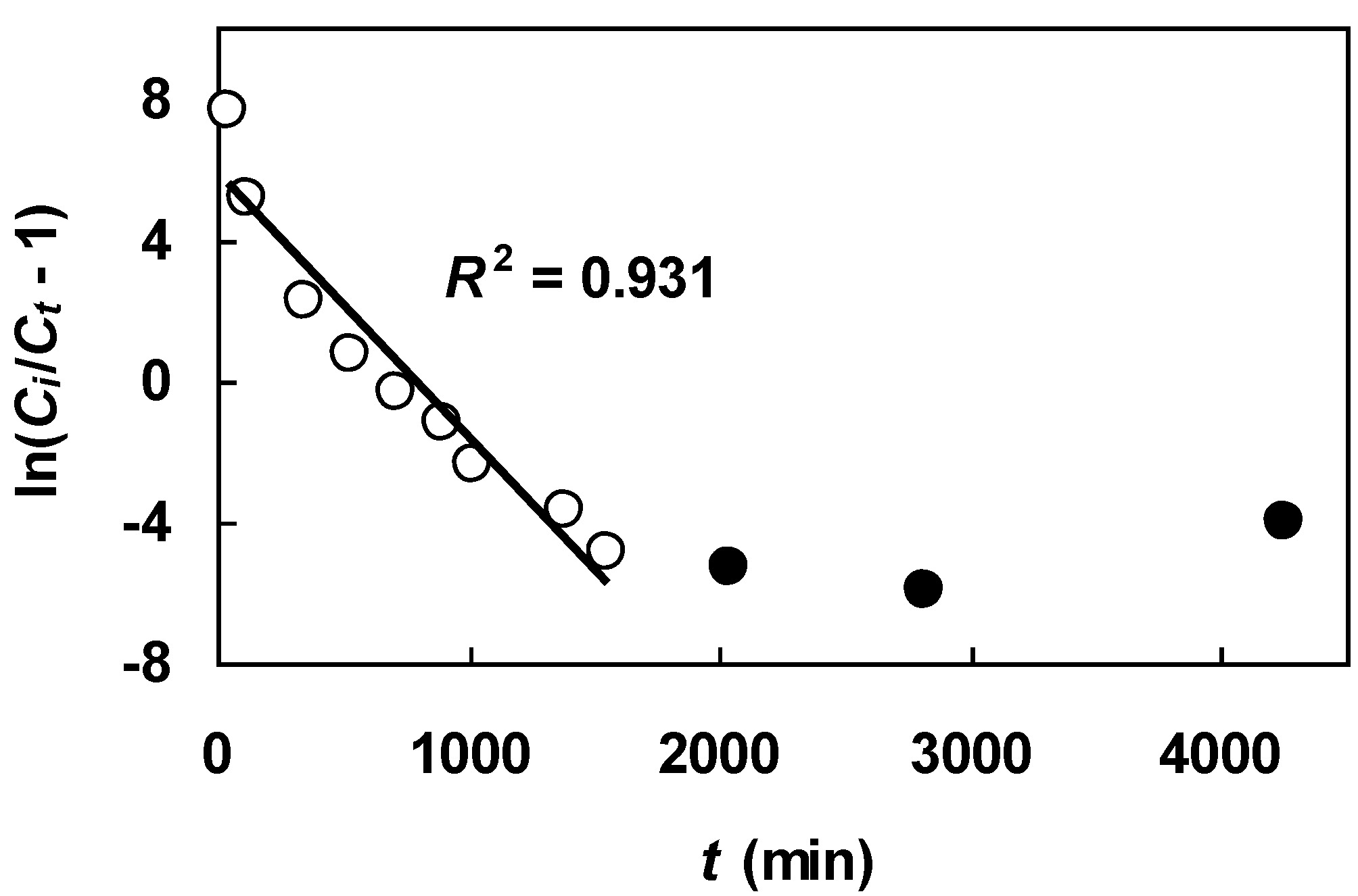
3.3.1. Bohart-Adams equation

In the Bohart-Adams fixed bed model it is assumed that the sorbate-sorbent interaction is represented by a quasi-chemical rate equation and that axial dispersion is zero [26,27]. A simplified version of the Bohart-Adams analytical solution is given by:

$$\frac{C_t}{C_i}=\frac{1}{1+\exp \left[\left(k_{BA}NZ\right)/u-k_{BA}{C}_{i}t\right]}$$

(11)

where C_t is the solution concentration at the fixed bed outlet at time t, C_i is the feed concentration, k_BA is the Bohart-Adams rate constant, N is the sorption capacity of the sorbent per unit volume of the bed, Z is the total bed depth, and u is the superficial velocity. In Equation (11) k_BA and N are fitting parameters. Equation (11) may be rearranged in the following manner to allow parameter estimation by linear regression:

$$\ln \left(\frac{C_i}{C_t}-1\right)=\frac{k_{BA}NZ}{u}-k_{BA}{C}_{i}t$$

(12)

from which it is evident that a plot of the left side of Equation (12) versus t should be linear. With known C_i, Z and u, the two parameters N and k_BA are given by the y-intercept and slope of the plot, respectively.

Figure 8 depicts the Figure 7 breakthrough data plotted according to Equation (12). It is clear that the transformed data did not conform to a linear trend. To get a linear fit, it was necessary to exclude the last three data points (filled circles in Figure 8). By this adjustment, a reasonably good fit was achieved, yielding an R² of 0.931. Listed in Table 6 are the values of N and k_BA obtained from the linear plot. The values of other variables, used in the calculation, are as follows: Z = 30.5 cm, C_i = 2.12 meq/L and u = 0.097 cm/min. Figure 9 compares the Figure 7 data with C_t/C_i calculated from the Bohart-Adams equation (Equation (11)) with the derived parameters (open circles). It can be seen that the Bohart-Adams equation containing the linear regression-generated parameters underestimated breakthrough concentrations in the low C_t/C_i region. This discrepancy is undesirable because the initial portion of a breakthrough curve determines the breakthrough time for a specified breakthrough concentration.

Figure 8. Breakthrough data in Figure 7 plotted according to the linearized Bohart-Adams equation (Equation (12)). Data points denoted by filled circles are excluded from the linear fit.

Figure 8. Breakthrough data in Figure 7 plotted according to the linearized Bohart-Adams equation (Equation (12)). Data points denoted by filled circles are excluded from the linear fit.

Table 6. Parameter estimation in the Bohart-Adams equation by the linear regression, nonlinear regression and GA methods.

Estimation method	N (meq/L)	kBA (L/meq min)	COD
Linear regression (Equation (12))	5.29	0.0035	0.963
Nonlinear regression	4.54	0.0029	0.998
Genetic algorithm	4.54	0.0029	0.998

Table 6. Parameter estimation in the Bohart-Adams equation by the linear regression, nonlinear regression and GA methods.

Estimation method	N (meq/L)	kBA (L/meq min)	COD
Linear regression (Equation (12))	5.29	0.0035	0.963
Nonlinear regression	4.54	0.0029	0.998
Genetic algorithm	4.54	0.0029	0.998

Figure 9. Comparison between the Figure 7 breakthrough data and C_t/C_i calculated from the Bohart-Adams equation (Equation (11)) with the linear regression-derived parameters (open circles) and GA-generated parameters (filled circles) tabulated in Table 6. Also shown are C_t/C_i calculated from the Belter-Cussler-Hu equation (Equation (13)) with the GA-derived parameters (triangles) given in Table 7.

Figure 9. Comparison between the Figure 7 breakthrough data and C_t/C_i calculated from the Bohart-Adams equation (Equation (11)) with the linear regression-derived parameters (open circles) and GA-generated parameters (filled circles) tabulated in Table 6. Also shown are C_t/C_i calculated from the Belter-Cussler-Hu equation (Equation (13)) with the GA-derived parameters (triangles) given in Table 7.

Next, the Bohart-Adams equation (Equation (11)) was fit to the Figure 7 data by using the GA and nonlinear regression methods. Table 6 shows that both techniques found equivalent parameter estimates. The COD was higher than that of the linear regression approach. As can be seen in Figure 9, values of C_t/C_i calculated from Equation (11) with the GA-derived parameters (filled circles) lie much closer to the 1:1 line for the entire data range. Even with a judicial selection of data points to aid the parameter estimation, the linear regression approach performed worse than the GA. This does not imply that the functional form of the Bohart-Adams equation is inadequate, merely that the suboptimal linear regression-derived parameters impair its correlative capability. An agreement between the Bohart-Adams equation and the breakthrough data can be reached as long as optimal parameter estimates are used in the equation.

For a typical breakthrough concentration ratio (C_t/C_i) of 0.1, the Bohart-Adams equation containing the linear regression-generated parameters predicts a breakthrough time of 488 min. From Figure 7 it is seen that the corresponding experimental breakthrough time is approximately 357 min. The predicted breakthrough time is thus 37% bigger than the observed breakthrough time. In contrast, a much better agreement can be obtained with the GA-derived parameters. In this case, the predicted breakthrough time for C_t/C_i = 0.1 is 313 min, which is only 13% smaller than the observed breakthrough time. From the foregoing discussion, it is clear that the linear regression approach yielded suboptimal parameters which can overestimate the breakthrough time substantially. Additionally, the linear regression approach relied on the use of a subset of the data points to achieve a good fit. The GA and nonlinear regression methods, by contrast, are free from these deficiencies. Despite its shortcomings, the linearized Bohart-Adams equation is a very popular modeling tool. Also shown in Figure 9 are results calculated from the Belter-Cussler-Hu equation (triangles), and these are discussed in the next section.

3.3.2. Belter-Cussler-Hu Equation

A semiempirical fixed bed model proposed by Belter et al. [28] is given by:

$$\frac{C_t}{C_i}=\frac{1}{2}\left[1+\text{erf}\left(\frac{t-t_c}{\sqrt{2}\sigma t_c}\right)\right]$$

(13)

where C_t, C_i, t are similarly defined in Equation (11) and t_c (characteristic time), σt_c (standard deviation) are parameters. The quantity erf(x) is the error function of x. Because the Belter-Cussler-Hu model is nonlinear in the parameters, t_c and σ can be found only by search. Equation (13) was fit to the Figure 7 data by using the nonlinear regression and GA methods. Both methods were equally successful in estimating the two parameters from the breakthrough data, as shown in Table 7. Comparing the COD statistics in Table 6 and Table 7 indicates that the Belter-Cussler-Hu equation was marginally better than the Bohart-Adams equation in correlating the breakthrough data. The same conclusion may be seen in Figure 9, which shows computed results of the Belter-Cussler-Hu equation (triangles) and those of the Bohart-Adams equation (filled circles).

Table 7. Parameter estimation in the Belter-Cussler-Hu equation by the nonlinear regression and GA methods.

Estimation method	tc (min)	σ	COD
Nonlinear regression	670.3	0.41	0.999
Genetic algorithm	670.3	0.41	0.999

Table 7. Parameter estimation in the Belter-Cussler-Hu equation by the nonlinear regression and GA methods.

Estimation method	tc (min)	σ	COD
Nonlinear regression	670.3	0.41	0.999
Genetic algorithm	670.3	0.41	0.999

Despite their comparable correlative power, the Belter-Cussler-Hu equation is far less popular than the Bohart-Adams equation. There is little doubt that the nonlinear nature of the Belter-Cussler-Hu equation is a major reason for its limited reach within the biosorption community. In a limited number of previous studies [29,30,31,32,33,34,35,36], nonlinear regression was used to fit the Belter-Cussler-Hu equation to experimental breakthrough data. Here we show that the GA is an effective alternative to the nonlinear regression approach.

4. Conclusions

Virtually all the mathematical models used to describe biosorption characteristics are inherently nonlinear; fitting the models to measured data therefore requires the use of iterative optimization techniques. To avoid the use of optimization methods, practitioners often select models that can be transformed to linearized forms so that model parameters can be obtained by linear regression. It is well known that using linearized versions of nonlinear models to correlate measured data can often lead to statistical deficiencies and inaccurate parameter estimates. Moreover, the bias towards models that can be linearized restricts the testing of models that cannot be linearized.

As can be seen from the analysis and results of this investigation, the genetic algorithm optimization method has proved very successful in fitting a variety of nonlinear isotherm, kinetic and fixed bed equations to experimental biosorption data. For models that can be linearized, the performance of the real-coded GA was superior to that of ordinary linear regression. In all the cases shown here, the correlative power of the GA was found to be comparable to that of nonlinear regression. Generally, gradient-based nonlinear regression techniques require initial parameter guesses that lie in the vicinity of the optimal values in order to avoid convergence difficulties while the GA method is able to minimize a nonlinear model within search ranges that vary over several orders of magnitude, so good initial guesses are not required. This was shown to be the case with the fitting of the three-parameter nth order rate equation. In conclusion, the GA has been demonstrated to be very effective as a parameter estimation tool in biosorption modeling, offering a useful alternative to standard nonlinear regression techniques.

References

1. Lesmana, S.O.; Febriana, N.; Soetaredjo, F.E.; Sunarso, J.; Ismadji, S. Studies on potential applications of biomass for the separation of heavy metals from water and wastewater. Biochem. Eng. J. 2009, 44, 19–41. [Google Scholar] [CrossRef]
2. Park, D.; Yun, Y.-S.; Park, J.M. The past, present, and future trends of biosorption. Biotechnol. Bioprocess Eng. 2010, 15, 86–102. [Google Scholar] [CrossRef]
3. Chojnacka, K. Biosorption and bioaccumulation—the prospects for practical applications. Environ. Int. 2010, 36, 299–307. [Google Scholar] [CrossRef] [PubMed]
4. McCuen, R.H.; Surbeck, C.Q. An alternative to specious linearization of environmental models. Water Res. 2008, 42, 4033–4040. [Google Scholar] [CrossRef] [PubMed]
5. Espinoza-Quiñones, F.R.; Módenes, A.N.; Costa, I.L., Jr.; Palácio, S.M.; Szymanski, N.; Trigueros, D.E.G.; Kroumov, A.D.; Silva, E.A. Kinetics of lead bioaccumulation from a hydroponic medium by aquatic macrophytes Pistia stratiotes. Water Air Soil Pollut. 2009, 203, 29–37. [Google Scholar] [CrossRef]
6. Espinoza-Quiñones, F.R.; Módenes, A.N.; Thome, L.P.; Palácio, S.M.; Trigueros, D.E.G.; Oliveira, A.P.; Szymanski, N. Study of the bioaccumulation kinetic of lead by living aquatic macrophyte Salvinia auriculata. Chem. Eng. J. 2009, 150, 316–322. [Google Scholar] [CrossRef]
7. Fiorentin, L.D.; Trigueros, D.E.G.; Módenes, A.N.; Espinoza-Quiñones, F.R.; Pereira, N.C.; Barros, S.T.D.; Santos, O.A.A. Biosorption of reactive blue 5G dye onto drying orange bagasse in batch system: kinetic and equilibrium modeling. Chem. Eng. J. 2010, 163, 68–77. [Google Scholar] [CrossRef]
8. Leitch, A.E.; Armstrong, P.B.; Chu, K.H. Characteristics of dye adsorption by pretreated pine bark adsorbents. Int. J. Environ. Stud. 2006, 63, 59–66. [Google Scholar] [CrossRef]
9. Holland, J.H. Adaptation in Natural and Artificial Systems; The University of Michigan Press: Ann Arbor, MI, USA, 1975. [Google Scholar]
10. Goldberg, D.E. Genetic Algorithms in Search, Optimization and Machine Learning; Addison-Wesley: New York, NY, USA, 1989. [Google Scholar]
11. Turkkan, N. Discrete optimization of structures using a floating-point genetic algorithm, Paper 134. In Annual Conference of the Canadian Society for Civil Engineering, Moncton, Canada, 4–7 June 2003.
12. Schiewer, S.; Balaria, A. Biosorption of Pb2+ by original and protonated citrus peels: equilibrium, kinetics, and mechanism. Chem. Eng. J. 2009, 146, 211–219. [Google Scholar] [CrossRef]
13. Langmuir, I. The adsorption of gases on plane surfaces of glass, mica, and platinum. J. Am. Chem. Soc. 1918, 40, 1361–1403. [Google Scholar] [CrossRef]
14. Bolster, C.H.; Hornberger, G.M. On the use of linearized Langmuir equations. Soil Sci. Soc. Am. J. 2007, 71, 1796–1806. [Google Scholar] [CrossRef]
15. Sweeney, M.W.; Melville, W.A.; Trgovcich, B.; Grady, C.P.L., Jr. Adsorption isotherm parameter estimation. J. Environ. Eng. Div. ASCE 1982, 108, 913–922. [Google Scholar]
16. Kinniburgh, D.G. General purpose adsorption isotherms. Environ. Sci. Technol. 1986, 20, 895–904. [Google Scholar] [CrossRef] [PubMed]
17. Freundlich, H. Kapilarchemie; Akademische Verlag: Leipzig, Germany, 1909. [Google Scholar]
18. Lagergren, S. Zur theorie der sogenannten adsorption gelöster stoffe. K. Sven. Vetenskapsakad. Handl. 1898, 24, 1–39. [Google Scholar]
19. Özer, A. Removal of Pb(II) ions from aqueous solutions by sulphuric acid-treated wheat bran. J. Hazard. Mater. 2007, 141, 753–761. [Google Scholar] [CrossRef] [PubMed]
20. Morais, W.A.; Fernandes, A.L.P.; Dantas, T.N.C.; Pereira, M.R.; Fonseca, J.L.C. Sorption studies of a model anionic dye on crosslinked chitosan. Colloids Surf. A 2007, 310, 20–31. [Google Scholar] [CrossRef]
21. Liu, Y.; Shen, L. A general rate law equation for biosorption. Biochem. Eng. J. 2008, 38, 390–394. [Google Scholar] [CrossRef]
22. Liu, Y.; Wang, Z.-W. Uncertainty of preset-order kinetic equations in description of biosorption data. Bioresourc. Technol. 2008, 99, 3309–3312. [Google Scholar] [CrossRef]
23. Brouers, F.; Sotolongo-Costa, O. Generalized fractal kinetics in complex systems (application to biophysics and biotechnology). Physica A 2006, 368, 165–175. [Google Scholar] [CrossRef]
24. Cooney, D.O. Adsorption Design for Wastewater Treatment; Lewis Publishers: Boca Raton, FL, USA, 1999. [Google Scholar]
25. Borba, C.E.; Guirardello, R.; Silva, E.A.; Veit, M.T.; Tavares, C.R.G. Removal of nickel(II) ions from aqueous solution by biosorption in a fixed bed column: Experimental and theoretical breakthrough curves. Biochem. Eng. J. 2006, 30, 184–191. [Google Scholar] [CrossRef]
26. Bohart, G.S.; Adams, E.Q. Some aspects of the behavior of charcoal with respect to chlorine. J. Am. Chem. Soc. 1920, 42, 523–529. [Google Scholar] [CrossRef]
27. Chu, K.H. Fixed bed sorption: setting the record straight on the Bohart-Adams and Thomas models. J. Hazard. Mater. 2010, 177, 1006–1012. [Google Scholar] [CrossRef] [PubMed]
28. Belter, P.A.; Cussler, E.L.; Hu, W.-S. Bioseparations: Downstream Processing of Biotechnology; Wiley: New York, NY, USA, 1988. [Google Scholar]
29. Brady, J.M.; Tobin, J.M.; Roux, J.C. Continuous fixed bed biosorption of Cu2+ ions: application of a simple two parameter mathematical model. J. Chem. Technol. Biotechnol. 1999, 74, 71–77. [Google Scholar] [CrossRef]
30. Stanley, L.C.; Ogden, K.L. Biosorption of copper (II) from chemical mechanical planarization wastewaters. J. Environ. Manage. 2003, 69, 289–297. [Google Scholar] [CrossRef] [PubMed]
31. Wong, K.K.; Lee, C.K.; Low, K.S.; Haron, M.J. Removal of Cu and Pb from electroplating wastewater using tartaric acid modified rice husk. Process Biochem. 2003, 39, 437–445. [Google Scholar] [CrossRef]
32. Chu, K.H. Improved fixed bed models for metal biosorption. Chem. Eng. J. 2004, 97, 233–239. [Google Scholar] [CrossRef]
33. Teng, M.-Y.; Lin, S.-H. Removal of basic dye from water onto pristine and HCl-activated montmorillonite in fixed beds. Desalination 2006, 194, 156–165. [Google Scholar] [CrossRef]
34. Lodeiro, P.; Herrero, R.; Sastre de Vicente, M.E. The use of protonated Sargassum muticum as biosorbent for cadmium removal in a fixed-bed column. J. Hazard. Mater. 2006, B137, 244–253. [Google Scholar] [CrossRef]
35. Ramirez, C.M.; Pereira da Silva, M.; Ferreira, L.S.G.; Vasco, E.O. Mathematical models applied to the Cr(III) and Cr(VI) breakthrough curves. J. Hazard. Mater. 2007, 146, 86–90. [Google Scholar] [CrossRef] [PubMed]
36. Lee, C.K.; Ong, S.T.; Zainal, Z. Ethylenediamine modified rice hull as a sorbent for the removal of basic blue 3 and reactive orange 16. Int. J. Environ. Pollut. 2008, 34, 246–260. [Google Scholar] [CrossRef]