Article

Assessing Watershed-Wildfire Risks on National Forest System Lands in the Rocky Mountain Region of the United States

1
Rocky Mountain Research Station, U.S. Forest Service, P.O. Box 7669, Missoula, MT 59807, USA
2
Pyrologix, LLC, 520 Ford St, Missoula, MT 59801, USA
3
Rocky Mountain Region, U.S. Forest Service, 740 Simms St, Golden, CO 80401, USA
*
Author to whom correspondence should be addressed.
Submission received: 12 April 2013 / Revised: 18 June 2013 / Accepted: 20 June 2013 / Published: 2 July 2013
(This article belongs to the Special Issue Ecological Watershed Management)

Abstract

:
Wildfires can cause significant negative impacts to water quality with resultant consequences for the environment and human health and safety, as well as incurring substantial rehabilitation and water treatment costs. In this paper we will illustrate how state-of-the-art wildfire simulation modeling and geospatial risk assessment methods can be brought to bear to identify and prioritize at-risk watersheds for risk mitigation treatments, in both pre-fire and post-fire planning contexts. Risk assessment results can be particularly useful for prioritizing management of hazardous fuels to lessen the severity and likely impacts of future wildfires, where budgetary and other constraints limit the amount of area that can be treated. Specifically we generate spatially resolved estimates of wildfire likelihood and intensity, and couple that information with spatial data on watershed location and watershed erosion potential to quantify watershed exposure and risk. For a case study location we focus on National Forest System lands in the Rocky Mountain Region of the United States. The Region houses numerous watersheds that are critically important to drinking water supplies and that have been impacted or threatened by large wildfires in recent years. Assessment results are the culmination of a broader multi-year science-management partnership intended to have direct bearing on wildfire management decision processes in the Region. Our results suggest substantial variation in the exposure of and likely effects to highly valued watersheds throughout the Region, which carry significant implications for prioritization. In particular we identified the San Juan National Forest as having the highest concentration of at-risk highly valued watersheds, as well as the greatest amount of risk that can be mitigated via hazardous fuel reduction treatments. To conclude we describe future opportunities and challenges for management of wildfire-watershed interactions.

1. Introduction

Provision of clean water is a fundamental ecosystem service provided by forested landscapes. In the western United States, much of the water supply originates on National Forest System lands [1]. Therefore, the maintenance and restoration of watershed health is a primary management objective of the U.S. Department of Agriculture Forest Service (Forest Service). Large and severe wildfires present a major threat to watershed health, because they can impair watershed condition, alter hydrologic and geomorphic processes, and ultimately degrade water quality [2,3,4,5]. Wildfires can lead to changes in flow regimes, flood frequency, erosion, and debris flows [6,7]. Wildfires can also lead to significant changes in stream water chemistry, and post-fire sediment-driven transport can lead to increases in contaminant loads [8,9,10,11]. In turn, water quality degradation can have significant consequences for human health, safety, and aquatic habitat, and can lead to substantial rehabilitation and water treatment costs. Water quality impacts can be of significant concern for water utilities, related not only to treatment costs and maintaining water quality standards, but also the potential for damage or impairment of infrastructure due to excessive sedimentation [7].
Thus there exists a need to assess watershed-wildfire risks across landscapes and to design risk mitigation strategies accordingly. In the post-fire context, burned area emergency response teams are interested in prioritizing watershed stabilization and rehabilitation efforts within the fire perimeter. In the pre-fire context, however, the exact timing and location of the wildfire are uncertain, requiring projections of watershed exposure and risk given current landscape conditions and patterns of historical fire occurrence and fire weather. A common pre-fire risk mitigation approach on federal lands in the western United States is hazardous fuels reduction treatments, which can be designed to lessen fire intensity and severity within treated areas [12], as well as to lessen the likelihood of fire reaching susceptible or sensitive locations outside of treated areas [13]. Limited budgets and millions of hectares requiring treatment create a need to systematically prioritize areas for treatment. Increasingly, geospatial risk-based analytical tools are providing a sound and systematic basis for assessment and prioritization efforts on federal lands in the United States and elsewhere [14,15], and more broadly for wildfire incident decision support [16].
Wildfire risk can be modeled and quantified as a composite function of fire likelihood, fire intensity, and the response of assessment endpoints to varying levels of exposure to fire [17,18]. A foundational component of spatial wildfire risk assessment is burn probability modeling [19,20,21,22], which attempts to capture spatial variability in fire likelihood and spread potential stemming from variation in possible ignition locations, weather patterns, topography, and fuel conditions [23,24,25]. Spatially explicit modeling of fire spread is especially critical for landscapes like the western U.S. where the predominant source of burning is fire spread from remotely ignited large fires rather than local ignitions. Geospatial overlays of burn probability modeling outputs with maps of natural and developed resources form the basis for probabilistic exposure analysis, which typically quantifies resource exposure in terms of burn probability, fireline intensity, flame length, and expected area burned [26,27]. A particularly relevant analysis quantified the exposure of municipal watersheds to wildfire on a National Forest in Montana, USA, illustrating vast differences in fire likelihood, fire behavior, and expected area burned, with significant implications for risk-based strategic fuels management [28].
Analysis of the effects of fire can then be coupled with modeled exposure levels, constituting the two primary components of wildfire risk assessment [18]. A variety of approaches can be employed to model fire effects, although a lack of broadly applicable process-based models, a recognition of scientific uncertainty surrounding fire effects, and a desire for a standard template that can be used for integrated assessment across a suite of natural and developed resources has led to a reliance on expert-defined “response functions” that characterize expected fire-related losses and benefits as a function of flame length [29,30]. The response function approach is a flexible platform that can account for additional environmental variables thought to influence response to fire and can therefore capture spatial variation in resource susceptibility and likely fire consequences [31]. Although there are process-based models that can predict the hydrological impacts of fire, to our knowledge none of these tools are designed to directly incorporate burn probability modeling outputs that capture spatial variation in wildfire likelihood and intensity, which is a key focus of this assessment.
In this article we present our use of state-of-the-art wildfire simulation and risk assessment techniques to perform a comparative assessment of watershed exposure and risk in the Rocky Mountain Region of the U.S. National Forest System. Our approach to wildfire simulation modeling improves upon existing methods for merging results across fire modeling landscapes by dampening “seam line” phenomena, as will be described. Our approach further uses geospatial data characterizing watershed susceptibility, enabling a refined spatial assessment of risk relative to using fire modeling outputs alone. Figure 1 outlines the major components of our assessment and mitigation framework, wherein watershed-wildfire risks are a function of wildfire likelihood, wildfire intensity, watershed location, and watershed erosion potential. The identification of areas suitable for fuel treatment then leads to the spatial delineation of risk mitigation opportunities. We will describe how watershed exposure and risk calculations can be used to inform prioritization of hazardous fuels and other risk mitigation efforts, and describe future opportunities and challenges for management of wildfire-watershed interactions.
Figure 1. Conceptual model of primary components of wildfire risk and risk mitigation assessment framework.
Water 05 00945 g001

2. Materials and Methods

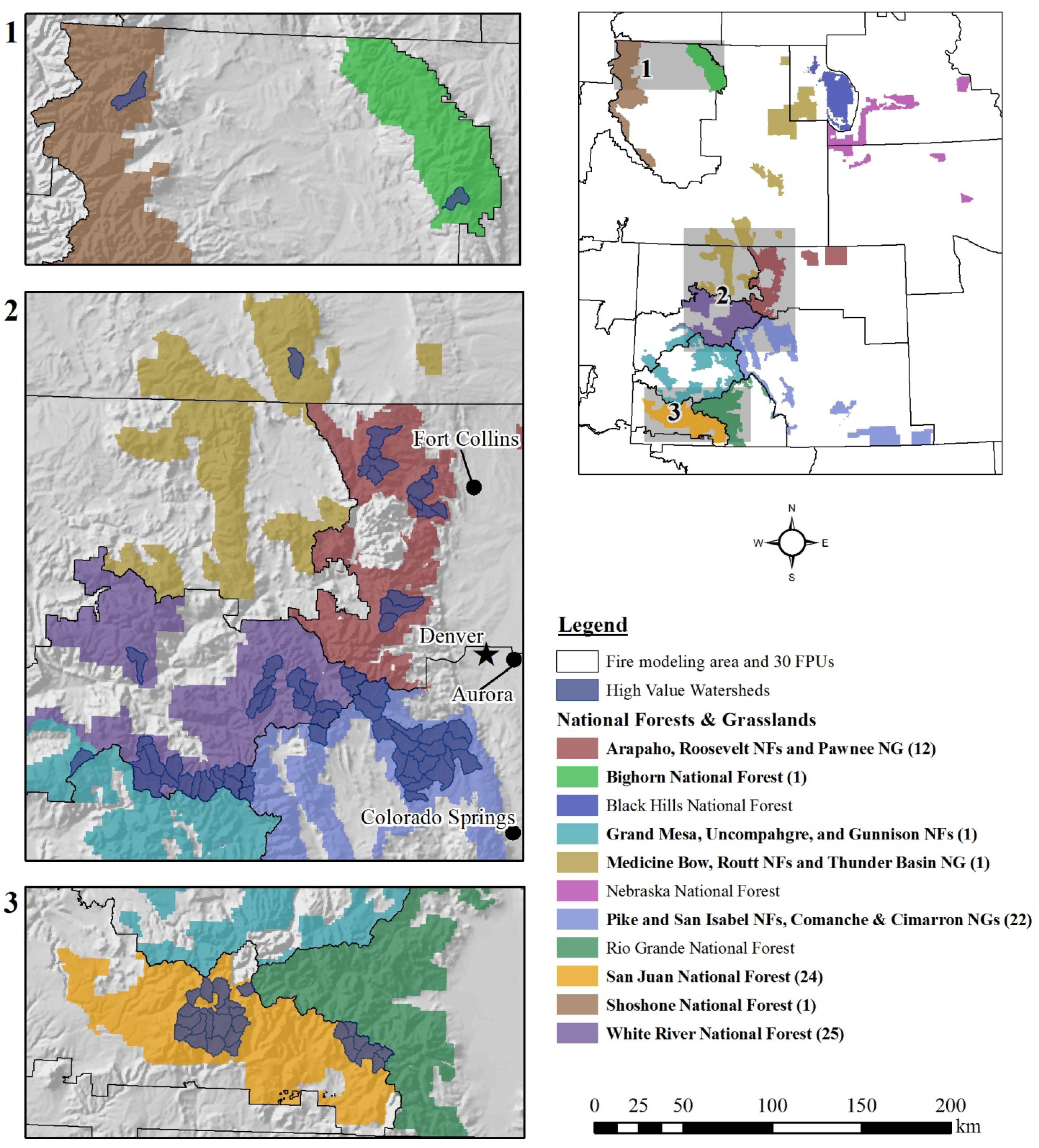
2.1. Case Study Location and Context

The Rocky Mountain Region provides a compelling study location, housing numerous high value watersheds that have been impacted or threatened by large wildfires in recent years [32]. Many of these watersheds contain or contribute to critically important reservoirs and watershed systems which provide drinking water to a large share of Colorado’s population; many of these watersheds are also located on National Forest System lands. Recent growth in human development and increased concerns over the impacts of future wildfire activity on water quality make this research particularly relevant.
Over the past two decades, the Region has experienced substantial wildfire-related impacts to critical watersheds, particularly in the Colorado Front Range Mountains. The Buffalo Creek Fire of 1996 burned 4800 ha of the Buffalo Creek watershed, destroying dwellings and leaving the vegetation highly susceptible to post-fire erosion. The Hayman Fire in 2002 burned approximately 56,000 ha more in the area, again leaving the basin vulnerable to damage from significant rain events. Subsequent rain events in these burned areas led to significant sediment accumulation—greater than 750,000 m3—in the Strontia Springs Reservoir, leading to significant costs—over $60 million for Denver Water and the Forest Service combined—for water treatment, sediment removal, reclamation, restoration, and watershed stabilization [33].
More recently, the 2012 fire season produced two large fires—again threatening water resources in the area. The High Park Fire burned 35,000 ha and, together with the Hewlett Gulch Fire earlier in the season, forced temporary diversion of Fort Collin’s water supply from the Poudre River to water from Horsetooth Reservoir fed by the Colorado River and Grand Lake portion of the water supply base [34]. The necessary treatment of the Poudre River water due to ash and particulate following the fire resulted in a water rate increase to Fort Collin’s residents. Further south, the Waldo Canyon Fire near Colorado Springs, burned 7000 ha around Rampart Reservoir—threatening water quality for the City of Colorado Springs and presenting additional costs for watershed rehabilitation and erosion mitigation [35]. The watershed health impacts caused by these fires, and concern over future wildfires prompted partnerships with federal and state agencies for investments in watershed protection and treatment of hazardous fuels. Denver Water Company and the Forest Service have entered into a partnership wherein matched funds totaling $33 million will be used for forest treatment and watershed protection [33].
Figure 2 illustrates the location of the Forest Service’s Rocky Mountain Region, which includes National Forests and Grasslands in the states of Colorado, Kansas, Nebraska, South Dakota, and Wyoming. In 2011, research scientists with the Forest Service’s Rocky Mountain Research Station engaged in a collaborative effort with the Rocky Mountain Region in order to perform a comprehensive wildfire risk assessment and to use those results to inform allocations of hazardous fuels budgets across Forests and Grasslands in the Region. In addition to watersheds, other resources and assets included in that original regional assessment include human communities, infrastructure (e.g., transmission lines), and critical habitat. When establishing priorities among these, regional leadership expressed a strong interest in watershed health and water quality, motivating the current study focusing specifically on assessment of watershed-wildfire risks.
For geospatial data on watersheds we turned to the Forest Service’s Forests to Faucets project [36], which models and maps the continental U.S. land areas most important to surface drinking water. Our specific interest was a data layer mapping the relative importance of all 12-digit Hydrologic Unit watersheds in the Region. Surface drinking water relative importance scores range from 0 to 100 and stem from an index derived from data on water supply, surface drinking water consumers at the point of intake, and the flow patterns to the surface water intakes. More information on the data sources and methods used to derive relative importance scores are provided in [36]. For our purposes we defined “high value watersheds” as the top 25% of watersheds by importance score as defined above, and for analysis purposes only assessed watersheds entirely contained within Forest Service boundaries (totaling 87 watersheds).
Figure 3 illustrates the location of these high value watersheds throughout the Region. Many of these watersheds are less than 80 km (50 miles) from Colorado’s most populous cities: Denver, Colorado Springs, Aurora, and Fort Collins. Most of the watersheds we assess are located throughout Colorado, with a few in Wyoming and none in the three eastern states. Of the 11 National Forests and Grasslands in the Region, 8 National Forests contain high value watersheds (listed alphabetically): Arapaho-Roosevelt; Bighorn; Grand Mesa, Uncompahgre and Gunnison; Medicine Bow-Routt, Pike-San Isabel; San Juan; Shoshone; and White River. None of the high value watersheds are located in National Grasslands.
Across the forested lands of the Region, vegetation compositions vary with elevation from the lower montane to subalpine zones. We used spatial layers from LANDFIRE [37], specifically Existing Vegetation Type and Fire Regime Group, to characterize the vegetation and historical fire regime expected in these watersheds. The large majority of selected watersheds are in higher-elevation subalpine forests typified by a mixture of subalpine fir (Abies lasiocarpa), lodgepole pine (Pinus contorta), aspen (Populus tremuloides), and Engelmenn spruce (Picea engelmanni). Mixed confiner forests make up the remaining majority of study area watersheds, with those in the higher elevations comprised of lodgepole pine, douglas fir (Psuedotsuga menziesii) and ponderosa pine (Pinus ponderosa), and those in lower elevations having a stronger ponderosa pine component. These characterizations are consistent with literature describing the forest types found in the Region [38,39]. There are three dominant fire regimes in this study area: (1) replacement severity with 35–200 year fire return interval; (2) low and mixed severity with 35–200 year fire return interval; and (3) low and mixed severity with ≤35 year fire return interval. One watershed, in the Bighorn National Forest in Wyoming, was characterized as a >200 year fire return interval at any severity.
Figure 2. National Forests and Grasslands in the Forest Service’s Rocky Mountain Region (CO = Colorado; KS = Kansas; NE = Nebraska; SD = South Dakota; WY = Wyoming).
Water 05 00945 g002
Figure 3. Fire modeling area (upper right box), with National Forest (NF) and Grassland (NG) boundaries and Fire Planning Unit (FPU) boundaries identified. The location and number of high value watersheds within each NF/NG are also identified (left three panels). Note that in the inset map state boundaries are not shown to allow for clearer presentation of FPU boundaries.
Water 05 00945 g003

2.2. Wildfire History and Simulation

Across the Rocky Mountain Region, between the years 1992–2011, large fires (>121 ha) burned approximately 2.5 million ha, accounting for 90% of all area burned, but only 2.4% of all fires [40]. Within National Forest System lands containing high value watersheds however, large fires comprise 1.2% of all fires and make up 97% of the area burned. Thus, our assessment of potential wildfire impacts to watersheds focused on those rare fires that grow to become very large under extreme fire weather.
We used the large-fire simulation system (FSim) [21] to simulate the occurrence, growth, and containment of fires on Forest Service and adjacent lands throughout the Region. FSim uses inputs related to the landscape (surface fuel, canopy fuel, forest vegetation, and topography), historical weather (fuel moisture, wind speed and wind direction) and historical fire occurrence (likelihood of large-fire occurrence in relation to fuel moisture) to simulate tens of thousands of fire seasons and provides results on both a per-fire and annual basis [21]. Simulation of a single fire season begins at the start of the large-fire season (an input) and proceeds day-by-day until large-fires no longer start and existing fires no longer spread. For each day, FSim determines whether to start one or more new fires based on the historical probability of large-fire occurrence. The number of large-fires to start is based on the historical distribution of number of large-fires per large-fire day. FSim simulates daily fire growth based on simulated fuel moisture and a random draw from the historical distribution of wind speed and direction. No fire spread is simulated if composite fuel moisture values falls below the year-long 80th percentile value. A containment module determines the likelihood that a simulated fire will be contained on a given day. If so, the fire is considered contained at its current size and will not grow on subsequent days of the season [21].
Primary outputs from FSim include pixel-level estimates of annual burn probability (BP), mean fireline intensity, and conditional flame length probabilities (binned into six flame length classes (FLCs; reported in English units): 0–2 ft, 2–4 ft, 4–6 ft, 6–8 ft, 8–12 ft, and 12+ ft), as well as polygon representations of simulated fire perimeters. Initially developed for national-scale assessment under the auspices of the interagency Fire Program Analysis (FPA) planning and budgetary system [41], FSim has since been used for myriad applications across a variety of geographic locations and planning scales [27,28,29,30,31,42]. The FPA wildfire simulations are conducted on pixelated (270 × 270 m2) landscapes, and parameterized and run at the scale of individual Fire Planning Units (FPUs) that are defined by FPA for the purposes of cooperative fire management planning and implementation. Spatial data inputs for the fire modeling landscape variables were obtained from LANDFIRE [37], and historical fire weather data from remote automated weather stations. FPUs range in size from approximately 1 to 6 million ha. For each FPU, FPA simulations were calibrated so that mean simulated BP was within the 95% confidence interval of the historical mean [21]. Compiling FPA simulation results across FPUs that span the Rocky Mountain Region, the simulated annual BP was 0.001480 relative to a historical value of 0.001506, and the simulated annual area burned was 110,873 ha relative to a historical value of 112,797 ha.
For this assessment we made two adjustments while stepping-down FPA’s most recent nationwide simulations to the regional level. First, we improved resolution by using FSim at a 180 m spatial resolution rather than 270 m. Second, we designed an alternative to FPA’s approach to generating a mosaic of separate FPU simulations. The FPA approach includes a 15 km buffer around each FPU, allowing fires to start in both the FPU and buffer area and spread into the FPU. The buffer is then removed and the results of adjacent FPUs compiled. With this approach, FSim’s fire intensity results (mean fireline intensity and flame length outputs) for pixels across adjacent FPU boundaries can be quite different, producing a seam line along FPU boundaries in the geospatial results. Such seam lines can exist if adjacent FPUs use significantly different wind speed, wind direction or fuel moisture inputs (FSim uses one input weather station data stream per FPU). This seam line modeling artifact can lead to perceptions that there are real world differences in fire occurrence and behavior patterns along FPU boundaries, when in fact, FPU boundaries are often defined along jurisdictional or other non-natural boundaries. The impact of these seam lines may be magnified for highly valued resources and assets that abut or cross FPU boundaries.
The fire modeling area for this assessment (Figure 3) is a rectangle (931 km east-west dimension by 1074 km north-south) that includes all Forest Service managed land in the Rocky Mountain Region plus a 60 km buffer, encompassing 100 million ha. The fire modeling area included all or part of 30 FPUs. We obtained LANDFIRE v1.1 fuel, vegetation and topography grids, at the native 30 m cell size, projected to NAD83 UTM Zone 13N projection, then resampled to a 180 m cell size. We generated 17 fire modeling landscape files (LCPs) to cover the fire modeling area; some LCPs could cover more than one FPU. Each LCP included a minimum 30 km buffer around the FPU for which it was to be used. The 30 km buffer was selected after recognizing that perimeters originating within FPU boundaries frequently grew larger than the 15 km buffer used by FPA. By doubling the buffered distance used by FPA combined with the 60 km forest buffer, we created a more natural transition in flame length outputs across FPU boundaries.
One input to FSim is a raster dataset that indicates the relative probability of a wildfire occurring across the fire modeling landscape, called an ignition density grid (IDG). The FPA program developed a nationwide IDG (25 km cell size) based on historical large-fire locations. FSim uses the IDG when locating simulated ignition points. We exploited this FSim input to develop an alternative method of compiling separate FSim runs for each FPU into an integrated result. We used the same IDG used by FPA, but modified it for each FPU simulation by setting the IDG value for a cell to zero for cells outside the FPU. This restricts FSim to ignition locations within the FPU. However, fires starting within the FPU can spread up to 30 km outside of it. Using this modified IDG would result in FSim placing the same number of fires as the FPA simulations into a smaller area. To ensure the correct number of fires relative to the FPA simulations, we adjusted the “AcreFract” FSim input. The AcreFract input is a linear adjustment factor on the number of simulated wildfires, originally designed to reflect the ratio of the total area of the fire modeling landscape to the land area for which historical fire occurrence data were actually available. That is, AcreFract inputs were adjusted to account for under-representation of limited or missing fire occurrence data for state, private, or other ownerships. In our case, we determined the appropriate AcreFract adjustment by summing the IDG values in the FPA landscape (which includes a 15 km buffer around each FPU) and dividing by the sum of IDG values in the portion of the FPU that occurs in the fire modeling area (without a buffer).
Because any given pixel can be burned by fires igniting in any adjacent FPU, the BP and fire intensity results required post-processing. Annual burn probability (BP) at a pixel is calculated as the sum of BP across all 30 FPU simulations.
Water 05 00945 i001
where BPk is the annual BP from the kth FPU at the pixel. Annual BP by flame length class (BPi) is calculated by weighting each FPU’s contribution to annual BP. FSim produces the conditional probability by flame length category (called the FLP, for flame length probability), so the calculation of BPi is:
Water 05 00945 i002
The implication of the BPi calculations is that the influence of the wind and fuel moisture from each FPU, which is determined from the historical weather recorded at a weather station representative of the FPU, is in proportion to how much each FPU contributes to BP. Near an FPU boundary there could be roughly equal representation of each FPU, but pixels further from the boundary will be more strongly influenced by one FPU than another. The result is a natural blurring of the intensity results near the FPU boundary, and a lessening of the potentially unrealistic seam line phenomenon.

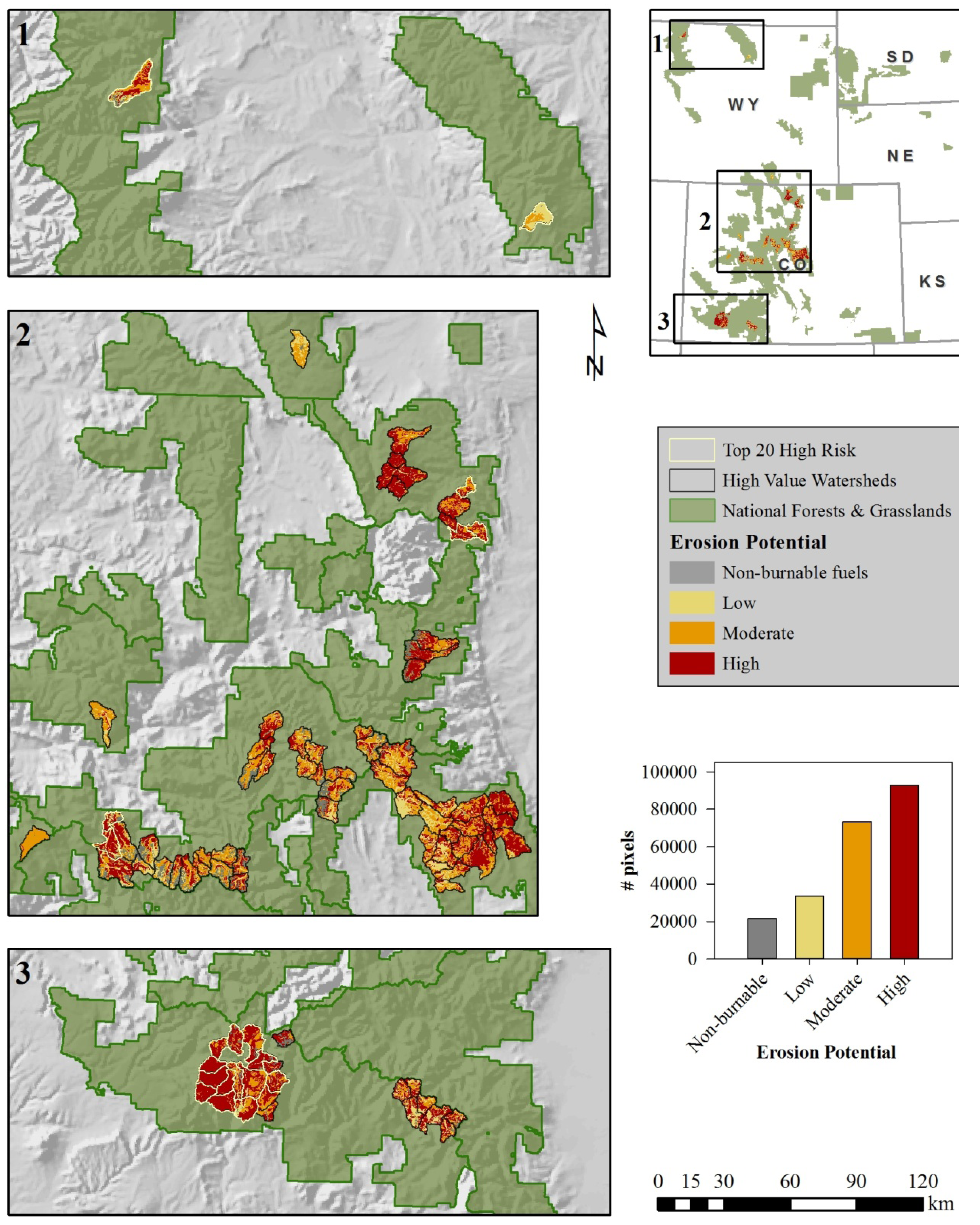
2.3. Erosion Potential

As described earlier, expert-based response functions can be designed to account for not only fire behavior characteristics but also landscape variables that could influence watershed susceptibility. Resource specialists with the Rocky Mountain Region identified erosion potential as a significant variable influencing likely post-fire sedimentation and water quality degradation. To characterize erosion potential we adopted methods described in the U.S. Department of Agriculture Natural Resources Conservation Service (NRCS) National Forestry Manual, Part 537: Soil Related Forest and Agroforestry Interpretations [43]. Our specific approach relied on the Potential Erosion Hazard (Off-Road/Off-Trail) criteria-based rating, which indicates the potential for soil loss after disturbance activities such as wildfire. The rating system yields four qualitative categories (slight, moderate, severe, and very severe) as a function of soil type and slope steepness.
Regional geospatial analysts compiled an erosion potential data layer combining forest-level data with NRCS Soil Survey data [44]. Erosion potential ratings are generally provided for individual soil components (including soil type and slope) that make up the soil mapping unit. Where the rating differed for various soil components within a soil mapping unit, we calculated a weighted average using the percent composition for each of the soil components. To calculate weighted averages we first generated a simple rubric for assigning numerical erosion potential scores: 0 (not rated, e.g., water); 1 (slight); 3 (moderate); and 5 (severe and very severe). Based upon weighted average calculations we then reclassified erosion potential indices in three bins: low (≤1.67), moderate (>1.67 and ≤3.33), or high (>3.33). We next used these bins for the purposes of categorical response function definition, as described in the following section.

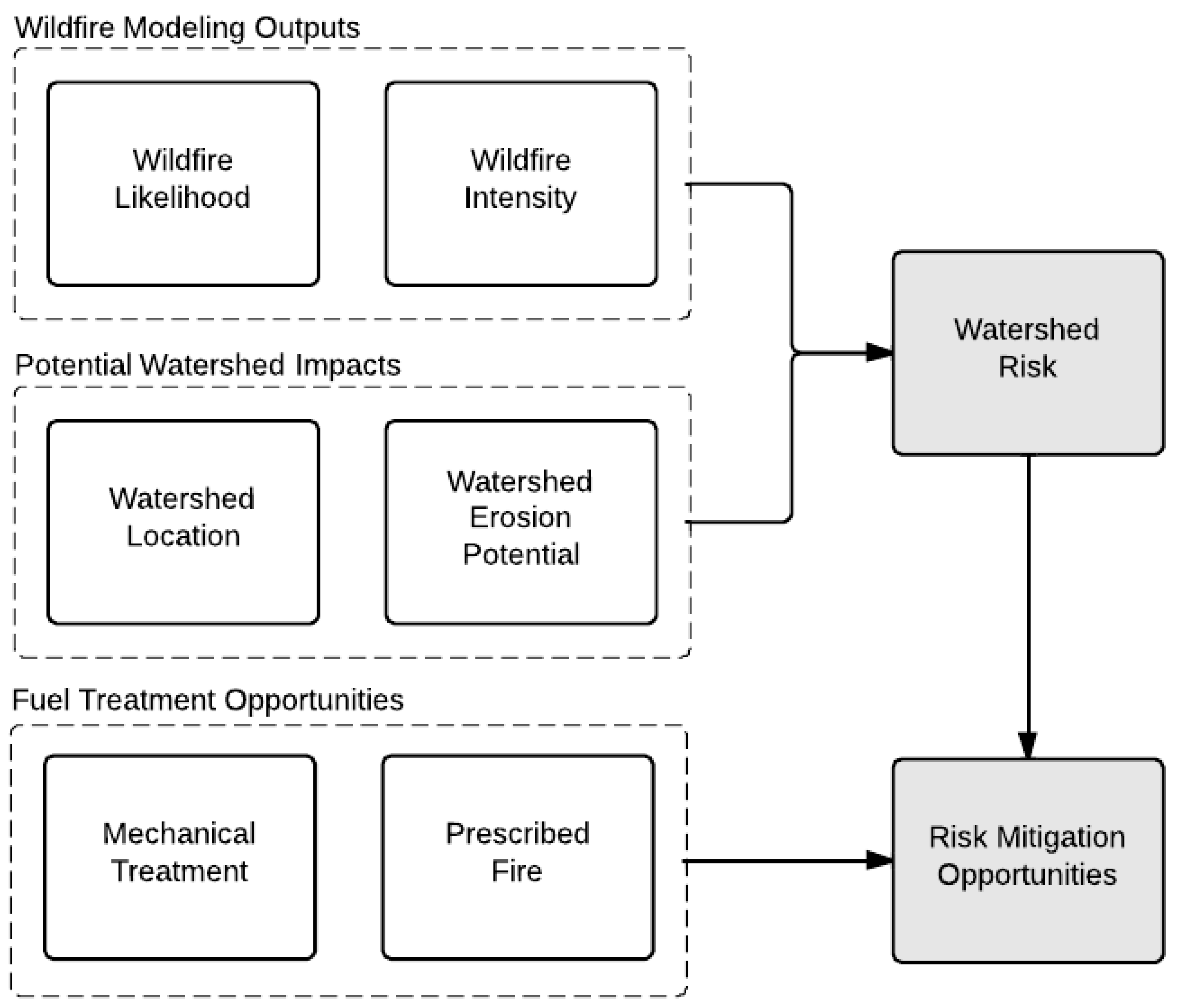
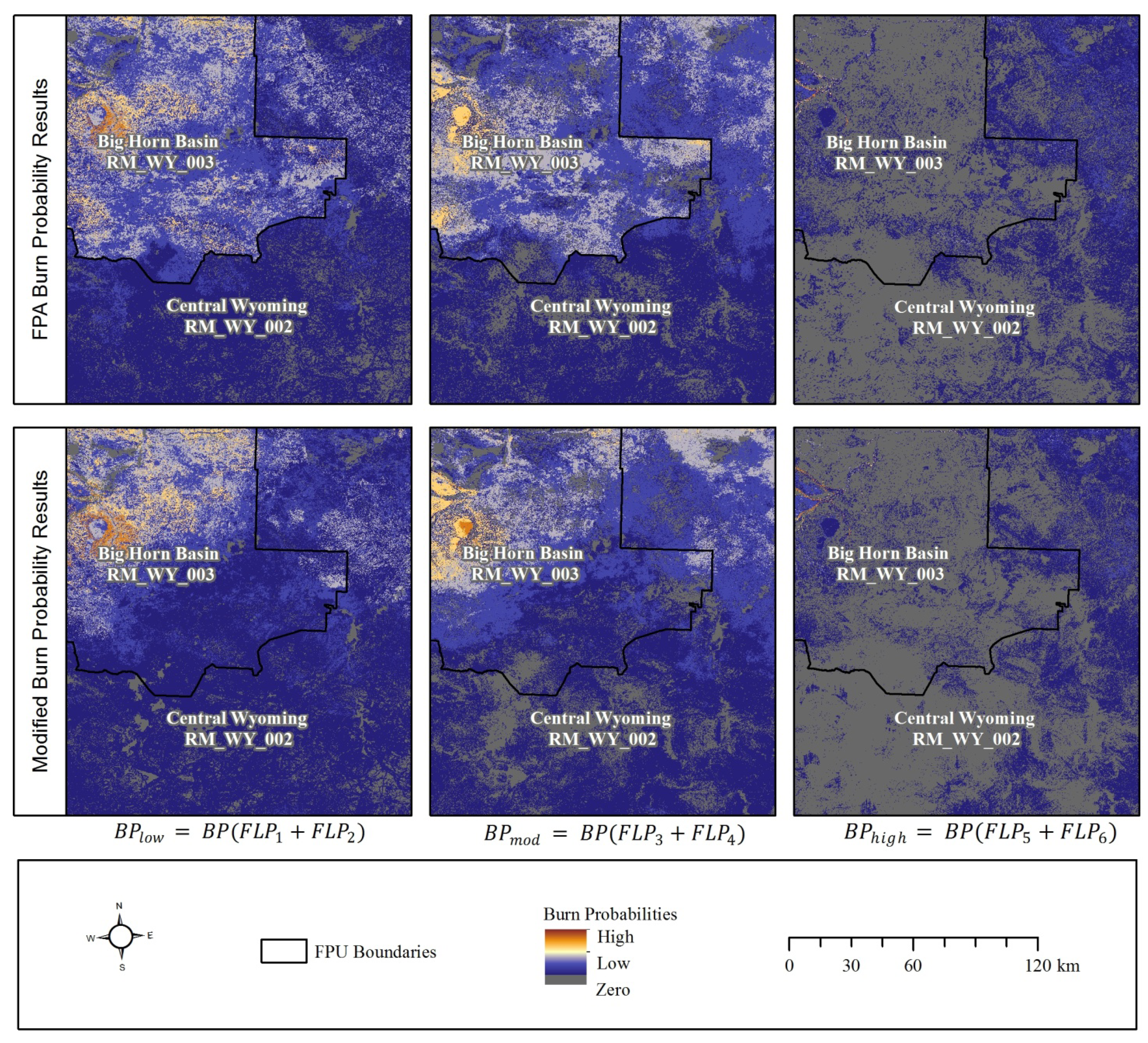
2.4. Wildfire Risk Assessment

The wildfire risk assessment framework we employ [18,31] quantifies risk in terms of expected net value change, or E(NVC). Results are calculated at the pixel level, which can be aggregated and summarized according to any polygon of interest (e.g., watershed, forest boundary). To geo-process risk calculations for all watersheds included in the assessment we used similar but more streamlined methods to those outlined in [30].
Expert-based response functions quantify net value change in relative terms ranging from −100% (complete loss) to +100% (maximum benefit). Where multiple socioeconomic and ecological resources are assessed, net value change results can be adjusted by weighting factors that reflect fire management priorities. Here we adopt a simpler approach that assumes all “high value” watersheds are of equal importance. Another adjustment to risk calculations relates to the mapped extent of watersheds, which normalizes net value change results according to the size of each watershed. We quantified E(NVC) for all watersheds as follows:
Water 05 00945 i003
where RFijl is the response function for watershed l at flame length class i at pixel j, and REl is the relative extent (watershed area) of watershed l.
To characterize exposure, we summarized BP and BPi metrics across all landscape pixels within watershed boundaries. This is primarily a geospatial exercise integrating fire modeling outputs with maps of the highly valued watersheds. Based on these pixel-level results, we calculated the expected annual watershed area burned by flame length category (EABi) for all watersheds using Equation (4):
Water 05 00945 i004
where Ap is the land area represented by a single pixel, and NW is the number of pixels in a given watershed. The overall expected watershed area burned (EAB) can be calculated as the sum of EABi values over the six flame length classes. Expected area burned represents the average amount of watershed area burned in a given year, and is driven largely by fire likelihood. These are simulated average values, and considerable variation from year to year in actual area burned can be expected (it may be likely that in most years no area of a given watershed will experience fire.)
Effects analysis is a more complicated effort, for which we adhered to a structured process for eliciting, synthesizing, and encapsulating expert judgment [31]. Reliance on expert judgment is often the best option for synthesizing available scientific knowledge, especially where assessments are time-sensitive and subject to uncertainty [45,46,47]. As part of the broader risk assessment, we held a full day workshop with Forest Service resource specialists who work for the Rocky Mountain Region, and who have expertise in fire ecology, soil science, and hydrology, among other disciplinary backgrounds. We asked these specialists to define response functions that provide estimates of net value change as a function of flame length and erosion potential.
Table 1 presents the multivariate response functions defined for and used in this analysis. Because our assessment effort does not model post-fire regeneration or vegetative succession through time, the response functions are short-term in temporal scope. These response functions focus on post-fire erosion and do not specifically model other concerns such as particulate emissions, although because sedimentation can deliver contaminants to stream these concerns are implicitly incorporated. The responses to fire have similar shapes across erosion potential classes, with expected losses monotonically increasing as flame length increases. Low intensity fires are considered neutral or modestly damaging, whereas with higher intensities the expectation is that burn severity, a primary determinant of watershed response, will also likely increase (recognizing that burn severity is influenced by a suite of factors beyond just fire intensity). Resource specialists identified areas with high erosion potential and high flame lengths to have the greatest potential for water quality degradation [2,3,4].
Table 1. Expert-defined response functions for fire effects to watersheds and surface drinking water quality. Numerical quantities in the table represent relative percentages of net value change for each erosion potential and flame length category.
Erosion Potential CategoryFlame Length Category
123456
0–2 feet2–4 feet4–6 feet6–8 feet8–12 feet12+ feet
Low00−10−20−30−30
Moderate0−10−20−30−40−50
High0−20−40−60−80−80

2.5. Prioritization and Mitigation Planning

The final step in our analysis was to generate information to facilitate the prioritization of areas for risk mitigation efforts. Here we focused on two spatial scales, providing exposure and risk rankings at the watershed as well as National Forest scale. Whereas the former may help identify particularly at-risk areas in need of treatment and help inform project planning at the forest level, the latter is more useful for budgetary planning at the regional level. The development of wildfire management strategies entails integrating risk assessment results with information on land and fire management objectives along with management opportunities and constraints (Figure 1). A critical factor to consider is the alignment of the spatiotemporal scope and evaluation criteria between the assessment and the broader decision process. The specific context of this assessment is a short-term risk assessment that relies on annual burn probability estimates and that is intended for informing annual allocation decisions and monitoring trends in risk over time.
One possible use of spatial risk assessment results is to guide post-fire mitigation planning. These results will likely be especially useful in the time period immediately after the wildfire, when fire severity measurements may not be available. The identified “hot spots” of high expected loss within burned areas can be given priority during field assessments of burn severity. When fire severity measurements are available the response functions can be rerun using the actual burn severity map rather than the FSim predictions. Flame length probabilities can help inform estimates of soil burn severity, which can in turn be used in post-fire erosion prediction tools [48]. A more in-depth analysis could first arrive at observation-based or worst-case estimates for flame length, and then re-run the tool over the burned area to identify areas of highest expected loss.
Another use of assessment results, which we focus on here, is for pre-fire planning and hazardous fuels reduction. This potential use of assessment results was in fact the primary reason for the collaborative science-management effort. As described above, developing risk mitigation strategies requires not only identification of high risk areas, but also which areas are suitable for fuel treatments. We relied on geospatial data provided by the Region that compiled spatial management area information stemming from individual National Forest and Grassland land management planning efforts. Specifically, we used two treatment filters, for mechanical treatment and for prescribed fire. Areas suitable for mechanical treatments are more restricted, due for instance to topographic limitations (slope steepness) as well as land designations such as Wilderness Areas in which mechanized equipment is prohibited. We then summarized risk rankings according to the highest levels of treatable risk.

3. Results and Discussion

3.1. Fire Modeling Landscape Characteristics

Figure 4 maps the BP values across the high value watersheds. The highest BPs occur in a watershed located in the Bighorn National Forest, with moderately high BPs also occurring in the watershed in the Shoshone National Forest and a cluster of watersheds in the southwestern corner in the San Juan National Forest. Elsewhere, BP values tend to be low.
Figure 4. Annual Burn Probability (BP) values mapped across the assessed high value watersheds [See Equation (1)]. The top 20 high risk watershed boundaries are highlighted. CO = Colorado; KS = Kansas; NE = Nebraska; SD = South Dakota; WY = Wyoming.
Water 05 00945 g004
Figure 5 similarly maps the variation in erosion potential across the assessed watersheds. Areas of high erosion potential are especially evident in the southwestern-most watersheds located in the San Juan National Forest. Scattered areas of moderate and high erosion potential are also evident along the Colorado Front Range in the Arapaho-Roosevelt National Forest, as well as in the Pike-San Isabel National Forest.
Figure 5. Erosion Potential categories mapped across the assessed high value watersheds, with the top 20 high risk watershed boundaries identified. CO = Colorado; KS = Kansas; NE = Nebraska; SD = South Dakota; WY = Wyoming.
Water 05 00945 g005

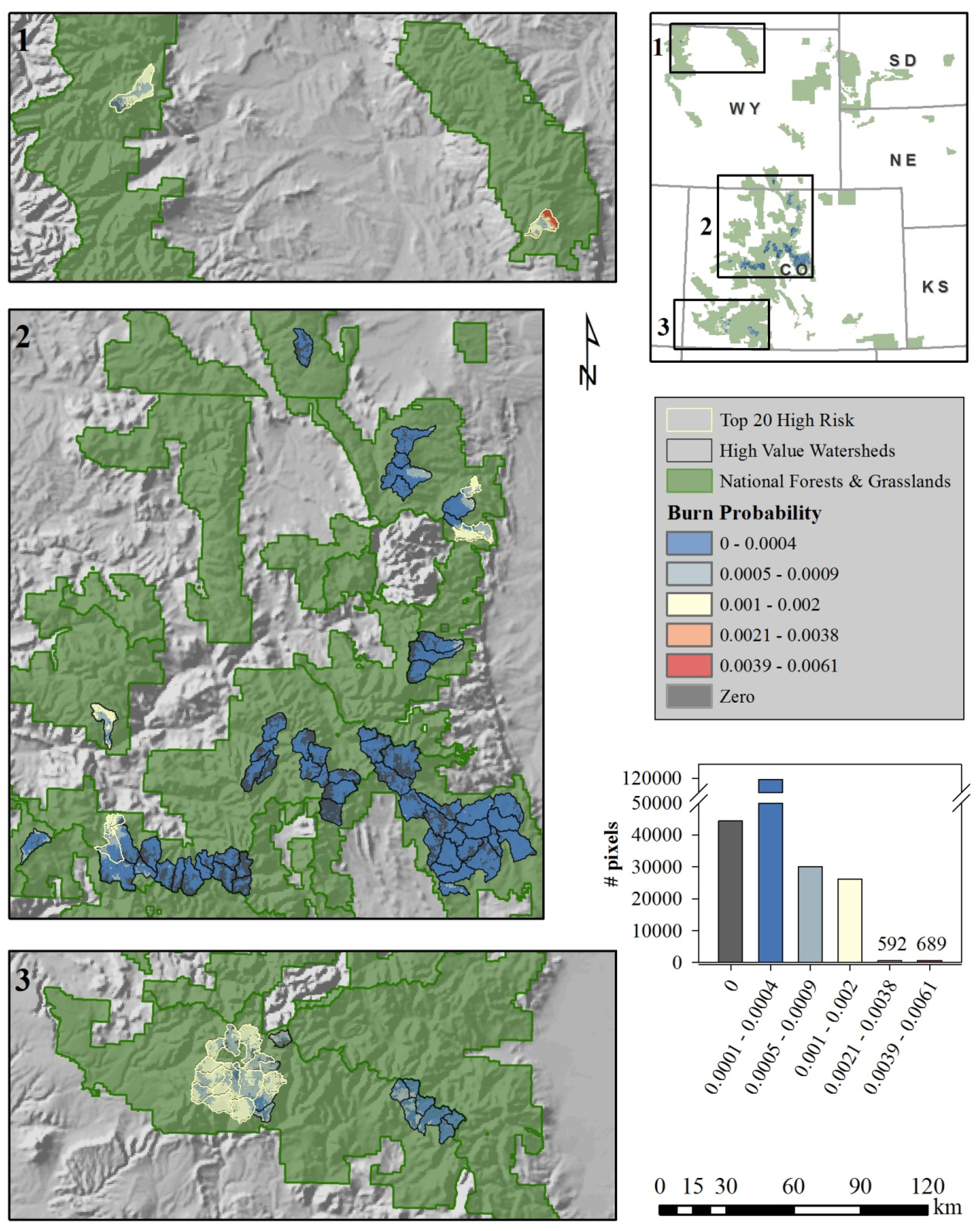
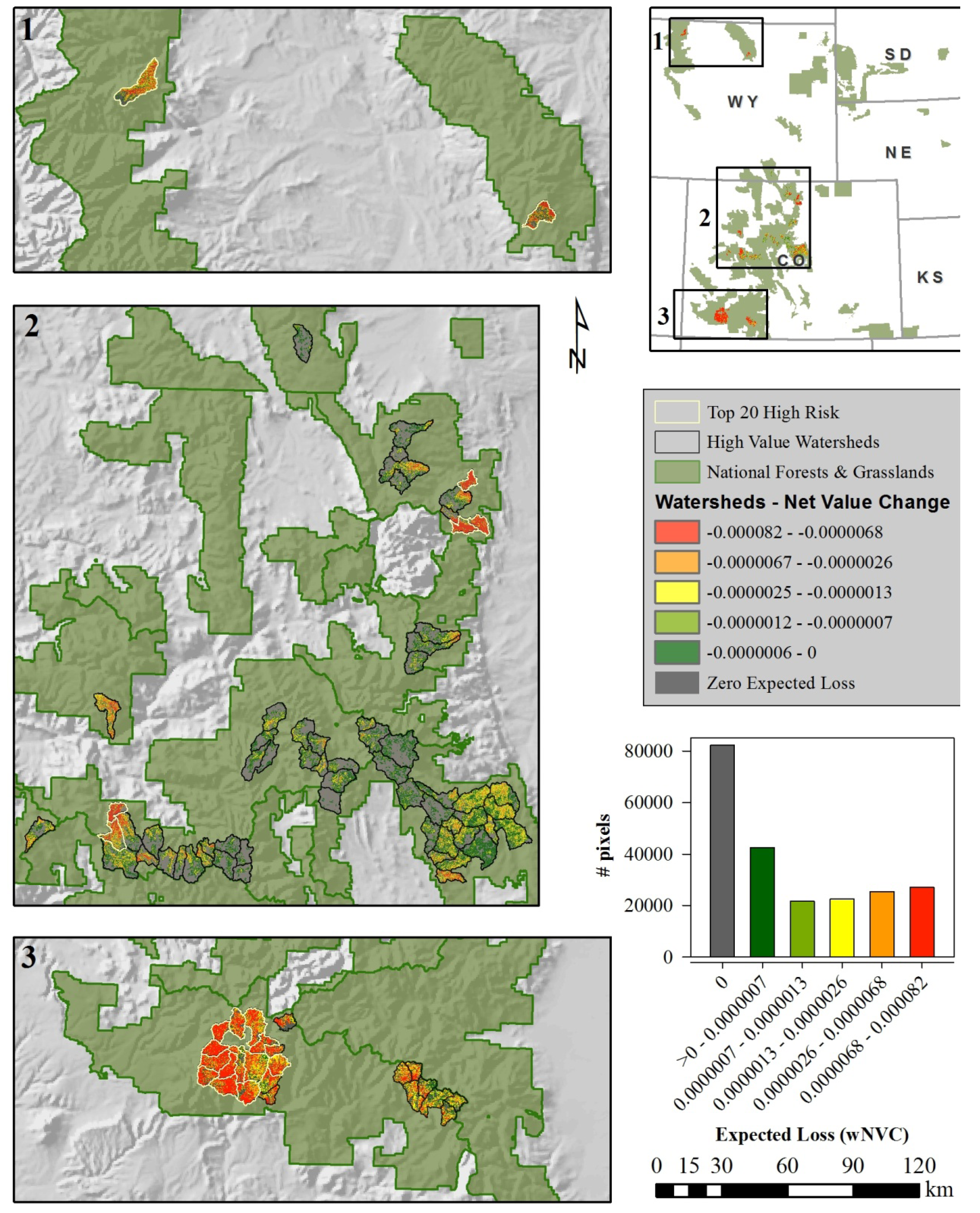
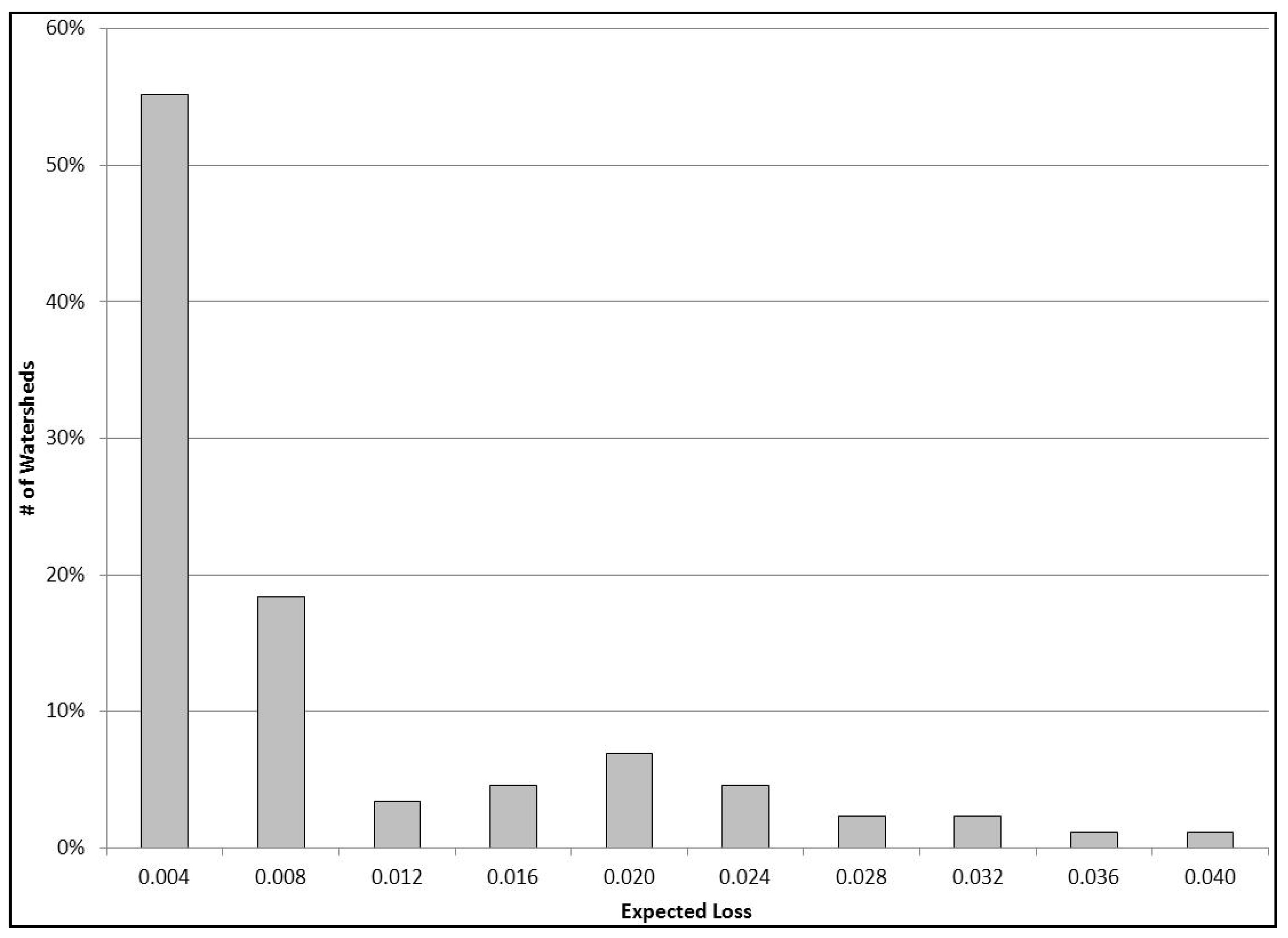
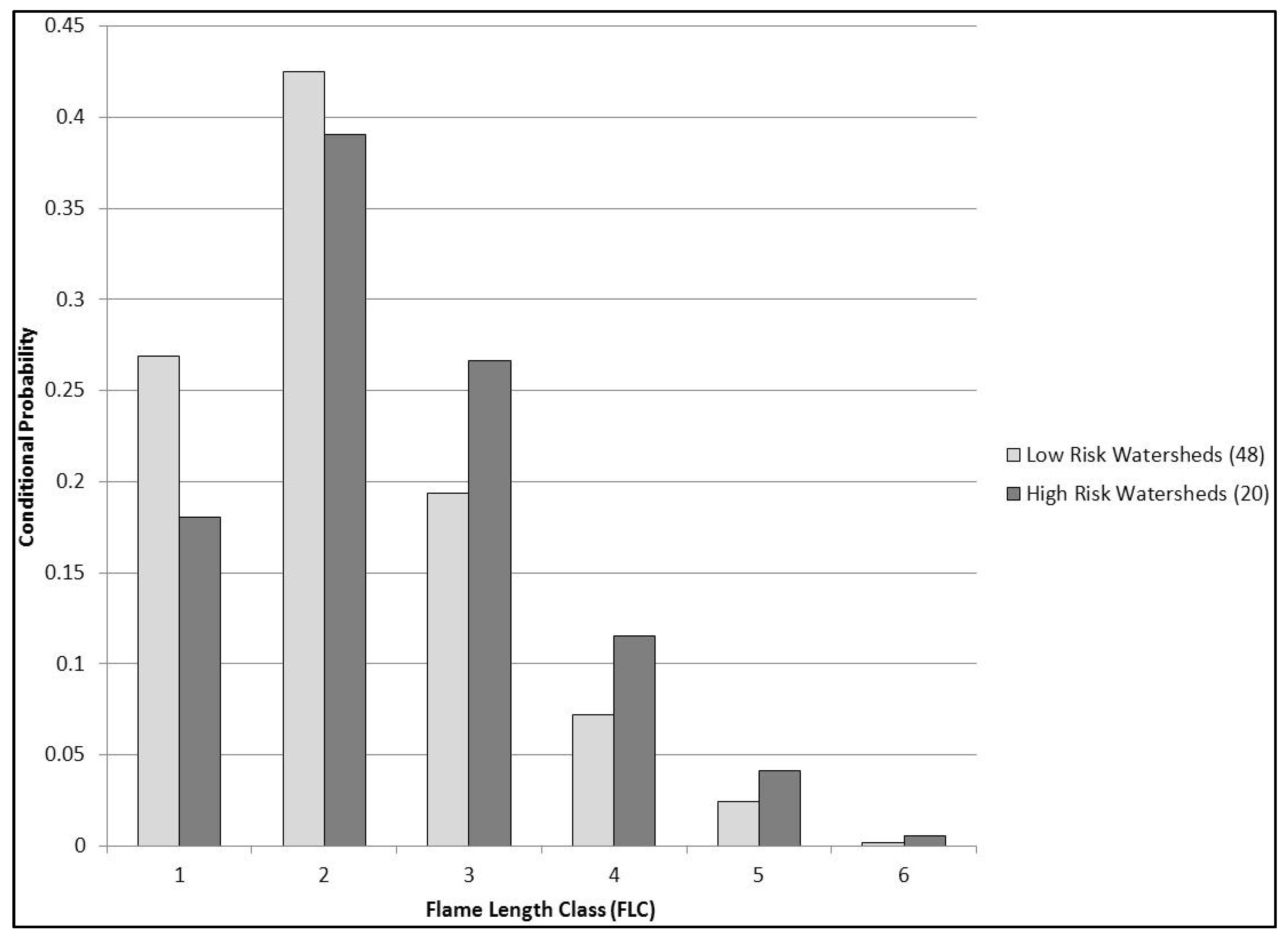
3.2. Watershed Exposure and Risk

Figure 6 maps expected net value change for all the watersheds we assessed. We present all risk outputs in terms of expected loss since the response function definitions were either neutral or damaging to watershed values; see Table 1. As might be expected from the information presented in Figure 4 and Figure 5, the southwestern-most watersheds present the highest levels of expected loss, due to the combination of relatively high BP and erosion potential.
Figure 6. Expected net value change (loss) mapped for the high value watersheds, with the top 20 high risk watersheds identified [See Equation (3)]. CO = Colorado; KS = Kansas; NE = Nebraska; SD = South Dakota; WY = Wyoming.
Water 05 00945 g006
Table 2 provides a ranked list of the 20 watersheds with the greatest expected loss. The table also provides information on mean watershed BP, watershed size, conditional watershed loss, erosion potential, and expected area burned. Conditional watershed loss relates to each watershed’s susceptibility if it were to experience fire, a function of the conditional distributions of flame length probability as well as erosion potential within the watershed. Conditional losses are obtained by dividing expected pixel-based losses values by pixel level BP, and then summarizing at the watershed level. The highest risk watershed has the highest conditional loss, due in large part to the vast majority of the watershed being in the highest erosion potential with associated larger potential for loss. Erosion potential is a primary factor driving conditional loss in our results, with a positive correlation of 0.71 between high erosion potential percentage and conditional loss across all 87 watersheds.
The correlation between conditional loss and expected loss drops to 0.63, reflecting the role of BP. BPi values for flame length classes (FLCs) 4–6 (Table 2), where losses are generally greater, exhibit a correlation with conditional loss of 0.70. By and large the flame length distributions are shifted to the left, with most of the expected area burned (84% on average for the top 20 watersheds; 88% overall) coming from FLCs 1–3. A notable exception is the 5th ranked watershed in the White River National Forest, where 34% of the expected area burned is from FLCs 4–6. The greater losses associated with higher fire intensities helps explain how a watershed with a relatively low value for total expected area burned can still rank high for expected loss.
As a general rule, watersheds with relatively high expected area burned have relatively high expected loss, although the rankings for total expected area burned do not match the rankings for expected loss. Across all 87 watersheds analyzed, the correlation between expected area burned and expected loss is 0.74. Divergence between expected loss and expected area burned can be explained in part by variable watershed size [NVC calculations are normalized by watershed area; Equation (3)], but as alluded to above this is mostly due to the multivariate response functions. For instance, although the watershed in the Bighorn National Forest (rank = 12) has by far the greatest amount of expected area burned, the majority burns at FLC 3 or lower, and because the watershed has mostly low erosion potential (Figure 5), the expected watershed response is dampened relative to other watersheds with less expected area burned but with higher erosion potential and/or higher flame length probabilities (Table 1).
Figure 7 presents a histogram of expected loss levels by watershed, sorted into 10 bins. The overwhelming majority of high value watersheds in the region present very low levels of expected loss. A total of 55.17% (48 of 87) of the watersheds have expected loss levels below 0.004, and a further 18.39% (16 watersheds) have expected loss levels below 0.008. The watersheds with the highest risk have expected losses that are orders of magnitude greater than low risk watersheds. These results indicate that many of the high value watersheds present minimal risk, due to spatial patterns of relatively low burn probabilities and relatively low erosion potential (Figure 4 and Figure 5). Figure 8 additionally compares conditional flame length probability distributions for the bottom 48 low risk watersheds and the top 20 high risk watersheds. Not only are the low risk watersheds less likely to burn (Figure 4), but when they do burn they tend to do so with lower intensity (Figure 8), thus leading to reduced expected loss.
Table 2. The top 20 at-risk watersheds, ranked according to expected (exp.) loss. Information is presented on watershed mean burn probability (BP), size, conditional (cond.) loss, erosion potential (in burnable areas), and expected area burned by flame length class (FLC).
Risk RankNational ForestExp. LossMean BPArea (ha)Cond. LossErosion Potential (%)Expected Area Burned (ha)
LMHFLC1FLC 2FLC 3FLC 4FLC 5FLC 6TotalRank
1San Juan0.03680.00125,68030.360.21.198.71.062.422.041.010.230.016.779
2San Juan0.03510.00138,69025.413.74.392.12.204.572.671.440.450.0311.363
3San Juan0.03180.00115,64129.100.711.188.20.802.261.880.860.200.026.0110
4San Juan0.02810.00108,56327.950.02.597.41.582.912.511.170.180.018.367
5White River0.02670.00094,23524.5832.512.954.60.231.561.080.630.670.194.3716
6Arapaho-Roosevelt0.02560.00105,39123.407.529.762.70.512.311.370.700.280.025.1913
7San Juan0.02380.00094,98324.410.525.873.70.931.501.690.550.100.004.7714
8San Juan0.02310.00138,63516.8817.024.958.11.845.922.330.800.250.0211.154
9San Juan0.02220.00095,93222.371.02.796.31.691.781.410.550.140.015.5811
10Arapaho-Roosevelt0.02050.00093,98820.423.559.537.00.371.421.260.530.140.013.7219
11San Juan0.01930.00109,81418.660.727.971.42.594.712.150.600.190.0310.286
12Bighorn0.01920.00239,3968.2567.832.00.22.618.776.312.710.970.2121.581
13Shoshone0.01910.000914,19819.0813.146.240.71.965.263.682.020.790.0713.792
14San Juan0.01850.00075,09022.805.53.191.30.871.490.800.490.240.033.9217
15Arapaho-Roosevelt0.01790.00084,87922.567.040.252.90.271.571.270.440.120.013.6720
16San Juan0.01680.000813,20020.234.235.860.12.503.743.000.970.260.0210.505
17San Juan0.01530.00086,26016.1214.330.455.31.142.261.420.390.090.015.3012
18San Juan0.01470.00106,58713.646.229.963.82.883.030.810.320.120.017.188
19San Juan0.01430.00066,16918.733.618.877.71.221.511.340.470.090.004.6315
20White River0.01280.00048,29825.1717.516.566.00.381.500.910.570.350.083.7918
Figure 7. Histogram of expected loss by watershed, presenting the total count of watersheds according to expected loss bins.
Water 05 00945 g007
Figure 8. Comparison of conditional probabilities by flame length class (FLC), for the bottom 48 low risk watersheds (1st column in Figure 6) and the top 20 high risk watersheds (4th–10th column in Figure 6; Table 2).
Water 05 00945 g008
Table 3 presents a ranked list of expected loss values across the 8 National Forests that contain high value watersheds. Generally, National Forests with a greater number of high value watersheds have a higher overall risk, as would be expected. The San Juan National Forest in particular stands out in terms of both expected area burned and expected loss relative to other National Forests in the Rocky Mountain Region.
Table 3. The National Forests with the greatest risk to watersheds and water quality, ranked according to expected loss [See Equations (3) and (4)].
Forest Risk RankNational ForestNumber of WatershedsExpected Area Burned (ha)Expected Loss
1San Juan24117.450.3696
2Arapaho and Roosevelt1226.160.0879
3White River2537.280.0864
4Pike-San Isabel2223.120.0483
5Bighorn121.580.0192
6Shoshone113.790.0191
7Grand Mesa, Uncompahgre and Gunnison12.700.0040
8Medicine Bow-Routt10.610.0005

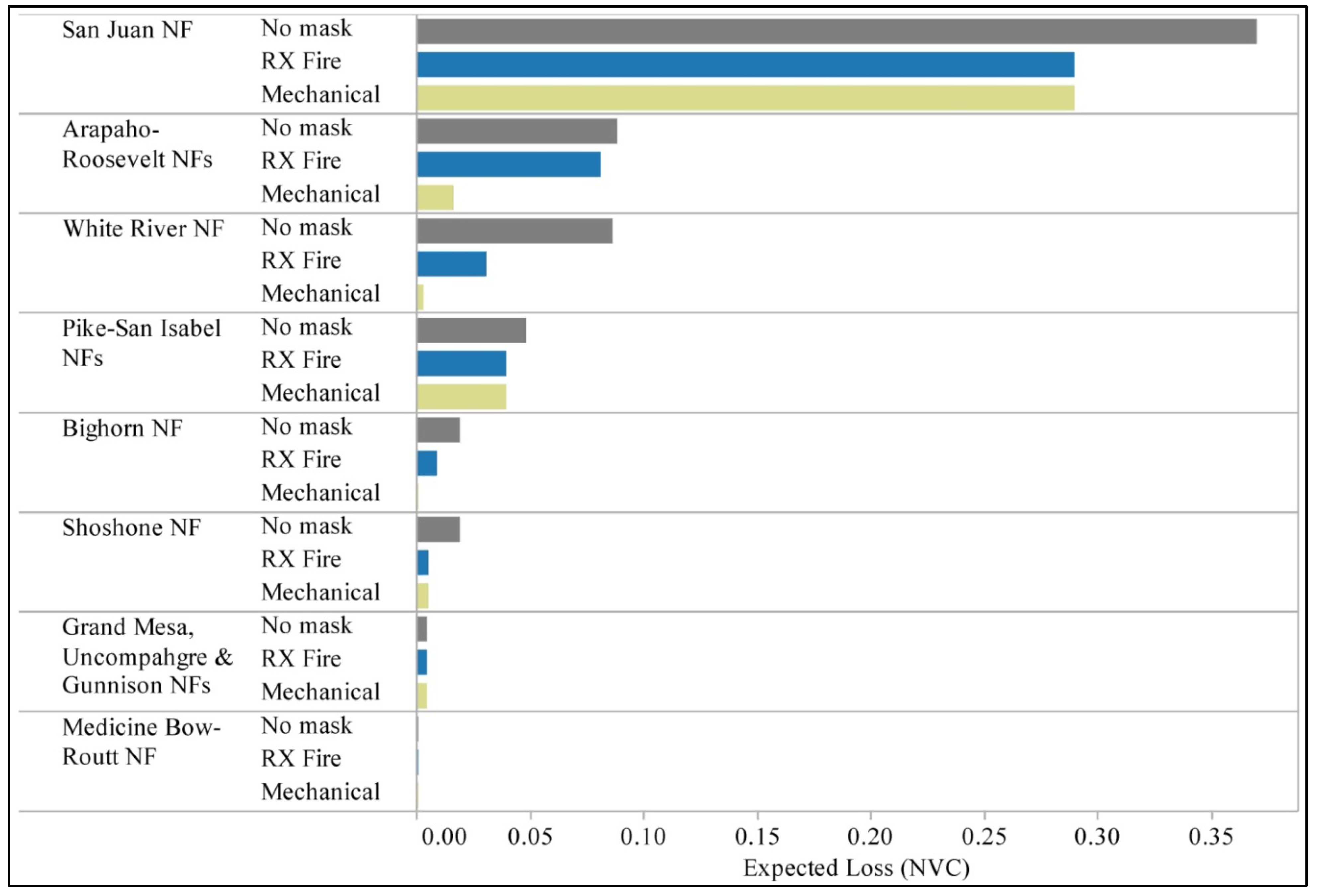
3.3. Watershed Risk Mitigation Opportunities

Figure 9 presents expected losses summarized at the forest-level, and further filtered according to areas suitable for prescribed fire or mechanical treatment. The unadjusted (no mask) results match those reported in Table 3; that is, the no mask results are total expected loss across both treatable and untreatable areas. In every National Forest, not all of the risk to high value watersheds is located in areas that can be treated. This disparity can help identify where investments in other risk mitigation activities beyond hazardous fuels reduction, particularly building initial attack response capacity, may be more efficient at reducing loss. The relative efficiency of such investments will depend on a suite of other factors not assessed here, including staffing levels, workforce training and qualifications, dispatch office locations, ownership patterns, firefighting resources, and transportation networks. Risk mitigation decisions of course will also depend on threats to other resources and assets, relative treatment opportunities, and managerial priorities.
Disparities in risk rankings and mitigation opportunities across Forests are also evident. For instance, although the White River National Forest has higher overall expected loss than the Pike-San Isabel National Forest, more of the risk can be mitigated on the Pike-San Isabel National Forest. In most cases there is an equal or lesser amount of risk that can be mitigated through mechanical treatment, highlighting the potential role for prescribed fire. However, real-world constraints associated with air quality, public and firefighter safety, and other concerns, may further limit prescribed fire opportunities. The results presented here provide a useful strategic overview for more detailed investigations into risk mitigation opportunities and challenges.
Figure 9. Expected loss summarized at the forest-level, and filtered according to spatial treatment opportunities [See Equation (3)]. RX Fire = Prescribed fire; NF = National Forest.
Water 05 00945 g009

3.4. FPU Weighting Approach

Although the emphasis of this paper is assessment of wildfire risk to watersheds, it is relevant to briefly compare simulated flame length probabilities across FPU boundaries using the original FPA approach and the approach we used here. Figure 10 compares flame length probability results across two FPUs located in the northwestern portion of the fire modeling landscape (Figure 3). Seam lines between the FPUs are more apparent when using FPA’s method (top panel) than with ours (bottom panel). Clearly, a seam line effect is still present even with our method, but it is significantly dampened, creating a more natural transition in fire intensities results. The overall effect of our weighting method depends on the distance wildfires burn across the FPU boundaries. Because FPUs are large relative to the sizes of the simulated wildfires, the zone of this natural weighting is relatively small, resulting in a reduction, but not elimination of seam lines.
Seam lines between FPUs are least prominent where the FPU boundary follows a significant, non-burnable landscape feature, like a tall mountain range whose upper reaches have insufficient fuel to support fire spread. In this study, the high-value watersheds near FPU boundaries happened to occur in such locations, so our FPU weighting method likely had little effect on the results. Nonetheless, we can recommend this method even for its slight improvement and more realistic representation of fire intensity transitions across FPU boundaries. The modified results align well with original FPA results: within the study area simulated annual BP was 0.000706 (relative to 0.000685), and simulated annual area burned was 5008 ha (relative to 4856 ha).
Figure 10. Comparison of unadjusted (top) and modified (bottom) FPA burn probability results. For display purposes fire modeling results are aggregated into three flame length probability (FLP) classes, and mapped across two FPU boundaries [See Equations (1) and (2)].
Water 05 00945 g010

3.5. Implications, Extensions and Limitations

Protecting watershed health and water quality from wildfire threats is a major management concern on National Forest System lands throughout the Rocky Mountain Region. Our results highlighted substantial variation in the exposure of and likely effects to highly valued watersheds throughout the Region, which carry significant implications for prioritization. In particular we identified the San Juan National Forest as having the highest concentration of at-risk highly valued watersheds in the Rocky Mountain Region, as well as the greatest amount of risk that can be mitigated via hazardous fuel reduction treatments.
Systematic application of a quantitative and geospatial wildfire risk assessment framework can lay the foundation for cost-effective mitigation of risks and restoration of landscapes, and further for monitoring exposure and risk trends through time. The joint identification of areas where risks are high and where risks can be treated will likely help guide future strategic fuels management efforts. Further, integrating risk assessment results into a broader structured decision making process could facilitate the evaluation of alternatives and examination of tradeoffs, and could ultimately help land managers decide on specific approaches to watershed management [49,50]. For instance, using response functions and maps of erosion potential, fire managers could target low-risk areas for implementation of low intensity prescribed fire. Comparative risk assessment could evaluate alternative fuel treatment strategies and their impact on future landscape conditions, and assessment results could be generated again to indicate changes in watershed exposure and risk. Policy tradeoffs could be examined as well, for instance asking whether the current agency focus on investing in fuel treatments near human development best achieves multiple land and resource objectives relative to other fuel treatment policies [51].
A number of potential expansions and extensions to this work are evident. The spatial scope of analysis could include a greater number of watersheds and a larger land base across federal, state, and private ownerships. The temporal scope of analysis could include potential long-term effects and broader landscape dynamics, in particular post-fire vegetation dynamics and their potential influence on the likelihood and/or magnitude of water quality impacts. Expanding the temporal scope of analysis even further could consider the potential impacts of a changing climate on both vegetation conditions and fire weather and occurrence. Modeling landscape dynamics through time however necessitates computational tradeoffs in terms of spatial resolution; in this case we were most interested in accurately capturing the spatial variability in watershed exposure and risk under current conditions. Of course, information on vegetation dynamics and recovery capacity could be brought into treatment prioritization decisions outside of the landscape risk assessment process, similar to the evaluation of management opportunity. In addition, at smaller planning scales more refined spatial data for modeling recovery capacity could be brought into assessments and project-level planning. At smaller scales it could also be possible to drill down into local land use history and determine potential impacts depending on the type and quantity of pollutants.
More immediate work relates to the modeling of watershed exposure and effects. A critical variable to capture is the areal extent of burning within a watershed. The current pixel-based approach however can only generate estimates of mean watershed area burned without capturing the associated variability. Moving beyond pixel-based estimates to include fire perimeter polygons in burn probability and area burned modeling in particular would be useful here [52,53]. This type of analysis would overlay simulated fire perimeters with watershed polygons, in order to generate conditional probability distributions for watershed area burned. Response functions could then be modified to account for both fire intensity and burned extent, and could potentially be defined to include threshold criteria for area burned, below which effects would be assumed negligible. Response functions could also include refined estimates of likely post-fire hillslope erosion [54].
Limitations of our assessment include uncertainties and errors surrounding fire simulations as well as response function definitions. Issues associated with fire modeling are discussed in more detail in [21,28], and issues associated with expert judgment elicitation are discussed in [31]. Careful attention to calibration, periodic critique and iterative refinement, and reliance on local knowledge and expertise are keystones of our modeling approach. As mentioned earlier, a better representation of both burn severity and the spatial extent of watershed area burned are critical for improving our understanding and ability to model the effects of fire on watershed health and water quality [55]. Broadly speaking however the risk modeling approaches employed here match well with the types of uncertainties faced [18], and present a robust and flexible approach to identifying, mapping, and prioritizing at-risk watersheds.

4. Conclusions

We presented application of an emerging geospatial wildfire risk assessment framework to quantify and map risks to watershed health and water quality, and further to help prioritize areas for risk mitigation efforts. The assessment is premised on explicitly modeling the spread of fire across the landscape, in order to capture spatial variation in wildfire likelihood and intensity and watershed exposure. Incorporating additional geospatial data on watershed susceptibility can also better capture spatial variation in watershed risk. Case study results did in fact evince substantial variation in expected loss across watersheds, and highlighted areas of particularly high risk that may be targeted for efficient mitigation investments.
The aims of this research were to facilitate an improved ability to understand the risks and mitigation opportunities across landscapes in the Rocky Mountain Region, and ultimately to foster an improved ability to make science-based land management decisions with the objectives of improving watershed and forest health. The fundamental assessment framework is flexible and scalable, and could thus provide utility to other land managers across ownerships and geographic areas. The framework is flexible in the sense that the primary analytical components of risk—exposure and effects—can be modeled and characterized in various ways. The framework is scalable in the sense that the spatial scope of analysis can vary from national to regional to forest-level to project-level. For instance, regional-scale planning may be concerned with prioritization and allocation decisions across forests, whereas forest-level planning may focus on smaller administrative units or specific watersheds. Suitability for various scales of analysis will vary according to the planning context and the availability of geospatial data.

Acknowledgments

We would like to thank the many individuals the Rocky Mountain Region who participated in this assessment, in particular the resource specialists who helped define response functions and members of regional leadership who helped articulate assessment endpoints and management priorities. Don Helmbrecht helped outline the fire modeling and assessment process, Karen Short provided assistance with fire modeling and fire history data, and Jim Menakis and Dave Calkin helped get the collaboration up and running. The National Fire Decision Support Center and the Rocky Mountain Research Station supported this effort.

Conflict of Interest

The authors declare no conflict of interest.

References

  1. Brown, T.C.; Hobbins, M.T.; Ramirez, J.A. Spatial distribution of water supply in the coterminous United States. J. Am. Water Res. Assoc. 2008, 44, 1474–1487. [Google Scholar] [CrossRef]
  2. Ice, G.G.; Neary, D.G.; Adams, P.W. Effects of wildfire on soils and watershed processes. J. For. 2004, 102, 16–20. [Google Scholar]
  3. Neary, D.G.; Ryan, K.C.; DeBano, L.F. Wildland Fire in Ecosystems: Effects of Fire on Soils and Water; General Technical Report RMRS-GTR-42-Vol.4; Rocky Mountain Research Station, USDA Forest Service: Ogden, UT, USA, 2005.
  4. Shakesby, R.A.; Doerr, S.H. Wildfire as a hydrological and geomorphological agent. Earth Sci. Rev. 2006, 74, 269–307. [Google Scholar] [CrossRef]
  5. Huey, G.M.; Meyer, M.L. Turbidity as an indicator of water quality in diverse watersheds of the Upper Pecos River Basin. Water 2010, 2, 273–284. [Google Scholar] [CrossRef]
  6. Oliver, A.A.; Reuter, J.E.; Heyvaert, A.C.; Dahlgren, R.A. Water quality response to the Angora Fire, Lake Tahoe, California. Biogeochemistry 2012, 111, 361–376. [Google Scholar] [CrossRef]
  7. Meixner, T.; Wohlgemuth, P. Wildfire impacts on water quality. Southwest Hydrol. 2004, 3, 24–25. [Google Scholar]
  8. Jung, H.Y.; Hogue, T.S.; Rademacher, L.K.; Meixner, T. Impact of wildfire on source water contributions in Devil Creek, CA: Evidence from end-member mixing analysis. Hydrol. Process. 2009, 23, 183–200. [Google Scholar] [CrossRef]
  9. Stein, E.D.; Brown, J.S.; Hogue, T.S.; Burke, M.P.; Kinoshita, A. Stormwater contaminant loading following southern California wildfires. Environ. Toxicol. Chem. 2012, 31, 2625–2638. [Google Scholar] [CrossRef]
  10. Stephens, S.L.; Meixner, T.; Poth, M.; McGurk, B.; Payne, D. Prescribed fire, soils, and stream water chemistry in a watershed in the Lake Tahoe Basin, California. Int. J. Wildland Fire 2004, 13, 27–35. [Google Scholar] [CrossRef]
  11. Burke, M.P.; Hogue, T.S.; Ferreira, M.; Mendez, C.B.; Navarro, B.; Lopez, S.; Jay, J.A. The effect of wildfire on soil mercury concentrations in Southern California watersheds. Water Air Soil Pollut. 2010, 212, 369–385. [Google Scholar] [CrossRef]
  12. Agee, J.K.; Skinner, C.N. Basic principles of forest fuel reduction treatments. For. Ecol. Manag. 2005, 211, 83–96. [Google Scholar] [CrossRef]
  13. Finney, M.A. A computational method for optimising fuel treatment locations. Int. J. Wildland Fire 2008, 16, 702–711. [Google Scholar] [CrossRef]
  14. Miller, C.; Ager, A.A. A review of recent advances in risk analysis for wildfire management. Int. J. Wildland Fire 2012, 22, 1–14. [Google Scholar] [CrossRef]
  15. Chuvieco, E.; Aguado, I.; Yebra, M.; Nieto, H.; Salas, J.; Martín, M.P.; Vilar, L.; Martínez, J.; Martín, S.; Ibarra, P.; et al. Development of a framework for fire risk assessment using remote sensing and geographic information system technologies. Ecol. Model. 2010, 221, 46–58. [Google Scholar] [CrossRef]
  16. Calkin, D.E.; Thompson, M.P.; Finney, M.A.; Hyde, K.D. A real-time risk assessment tool supporting wildland fire decisionmaking. J. For. 2011, 109, 274–280. [Google Scholar]
  17. Finney, M.A. The challenge of quantitative risk analysis for wildland fire. For. Ecol. Manag. 2005, 211, 97–108. [Google Scholar] [CrossRef]
  18. Thompson, M.P.; Calkin, D.E. Uncertainty and risk in wildland fire management: A review. J. Environ. Manag. 2011, 92, 1895–1909. [Google Scholar] [CrossRef]
  19. Bar Massada, A.; Radeloff, V.C.; Stewart, S.I.; Hawbaker, T.J. Wildfire risk in the wildland-urbaninterface: A simulation study in northwestern Wisconsin. For. Ecol. Manag. 2009, 258, 1990–1999. [Google Scholar] [CrossRef]
  20. Finney, M.A.; Grenfell, I.C.; McHugh, C.W.; Seli, R.C.; Tretheway, D.; Stratton, R.D.; Brittain, S. A method for ensemble wildland fire simulation. Environ. Model. Assess. 2011, 16, 153–167. [Google Scholar] [CrossRef]
  21. Finney, M.A.; McHugh, C.W.; Stratton, R.D.; Riley, K.L. A simulation of probabilistic wildfire risk components for the continental United States. Stoch. Environ. Res. Risk Assess. 2011, 25, 973–1000. [Google Scholar] [CrossRef]
  22. Ager, A.A.; Vaillant, N.M.; Finney, M.A.; Preisler, H.K. Analyzing wildfire exposure and source-sink relationships on a fire prone forest landscape. For. Ecol. Manag. 2012, 267, 271–283. [Google Scholar] [CrossRef]
  23. Parks, S.A.; Parisien, M.A.; Miller, A. Spatial bottom-up controls on fire likelihood vary across western North America. Ecosphere 2012, 3. Article 12. [Google Scholar]
  24. Parisien, M.A.; Miller, C.; Ager, A.A.; Finney, M.A. Use of artificial landscapes to isolate controls on burn probability. Landsc. Ecol. 2010, 25, 79–93. [Google Scholar] [CrossRef]
  25. Parisien, M.A.; Walker, G.R.; Little, J.M.; Simpson, B.N.; Wang, X.; Perrakis, D.D.B. Considerations for modeling burn probability across landscapes with steep environmental gradients: An example from the Columbia Mountains, Canada. Nat. Hazards 2013, 66, 439–462. [Google Scholar] [CrossRef]
  26. Salis, M.; Ager, A.A.; Arca, B.; Finney, M.A.; Bacciu, V.; Duce, P.; Spano, D. Assessing exposure of human and ecological values to wildfire in Sardinia, Italy. Int. J. Wildland Fire 2012, 22, 549–565. [Google Scholar]
  27. Ager, A.A.; Buonopane, M.; Reger, A.; Finney, M.A. Wildfire exposure analysis on the National Forests in the Pacific Northwest, USA. Risk Anal. 2013, 33, 1000–1020. [Google Scholar] [CrossRef]
  28. Scott, J.; Helmbrecht, D.; Thompson, M.P.; Calkin, D.E.; Marcille, K. Probabilistic assessment of wildfire hazard and municipal watershed exposure. Nat. Hazards 2012, 64, 707–728. [Google Scholar] [CrossRef] [Green Version]
  29. Thompson, M.P.; Calkin, D.E.; Gilbertson-Day, J.; Ager, A.A. Advancing effects analysis for integrated, large-scale wildfire risk assessment. Environ. Monit. Assess. 2011, 179, 217–239. [Google Scholar] [CrossRef]
  30. Thompson, M.P.; Calkin, D.E.; Finney, M.A.; Ager, A.A.; Gilbertson-Day, J.W. Integrated national-scale assessment of wildfire risk to human and ecological values. Stoch. Environ. Res. Risk Assess. 2011, 25, 761–780. [Google Scholar] [CrossRef]
  31. Thompson, M.P.; Scott, J.; Helmbrecht, D.; Calkin, D.E. Integrated wildfire risk assessment: Framework development and application on the Lewis and Clark National Forest in Montana, USA. Integr. Environ. Assess. Manag. 2013, 9, 329–342. [Google Scholar] [CrossRef]
  32. Rhoades, C.C.; Entwistle, D.; Butler, D. The influence of wildfire extent and severity on streamwater chemistry, sediment and temperature following the Hayman Fire, Colorado. Int. J. Wildland Fire 2011, 20, 430–442. [Google Scholar] [CrossRef]
  33. Denver Water Web Page. From Forests to Faucets: U.S. Forest Service and Denver Water Watershed Management Partnership. Available online: http://www.denverwater.org/supplyplanning/watersupply/partnershipUSFS/ (accessed on 4 May 2013).
  34. Magill, B. Potential for Catastrophic Fire Threatens Fort Collins Water Supply. Available online: http://www.coloradoan.com/article/20130330/NEWS01/303300032/Potential-catastrophic-fire-threatens-Fort-Collins-water-supply (accessed on 4 May 2013).
  35. Eichenseher, T. Colorado Wildfires Threaten Water Supplies. Available online: http://news.nationalgeographic.com/news/2012/07/120703/colorado-wildfires-waldo-high-park-hayman-threaten-water-supplies/ (accessed on 4 May 2013).
  36. USDA Forest Service. Forests to Faucets. Available online: http://www.fs.fed.us/ecosystemservices/FS_Efforts/forests2faucets.shtml (accessed on 30 January 2013).
  37. Ryan, K.C.; Opperman, T.S. LANDFIRE—A national vegetation/fuels data base for use in fuels treatment, restoration, and suppression planning. For. Ecol. Manag. 2013, 294, 208–216. [Google Scholar] [CrossRef]
  38. Sibold, J.S.; Veblen, T.T.; González, M.E. Spatial and temporal variation in historic fire regimes in subalpine forests across the Colorado Front Range in Rocky Mountain National Park, Colorado, USA. J. Biogeogr. 2006, 32, 631–647. [Google Scholar]
  39. Schoennagel, T.; Veblen, T.T.; Romme, W.H. The interaction of fire, fuels, and climate across Rocky Mountain forests. BioScience 2004, 54, 661–676. [Google Scholar] [CrossRef]
  40. Short, K. Personal communication. U.S. Forest Service Rocky Mountain Research Station: Missoula, MT, USA, June 2013. [Google Scholar]
  41. Forests and Rangelands Web Page. Fire Program Analysis (FPA). Available online: http://www.forestsandrangelands.gov/FPA/index.shtml (accessed on 30 January 2013).
  42. Thompson, M.P.; Vaillant, N.M.; Haas, J.R.; Gebert, K.M.; Stockmann, K.D. Quantifying the potential impacts of fuel treatments on wildfire suppression costs. J. For. 2013, 111, 49–58. [Google Scholar]
  43. U.S. Department of Agriculture Natural Resources Conservation Service, National Forestry Manual; U.S. Department of Agriculture: Washington, DC, USA, 1998; Available online: ftp://ftp-fc.sc.egov.usda.gov/NSSC/National_Forestry_Manual/2002_nfm_complete.pdf (accessed on 4 May 2013).
  44. U.S. Department of Agriculture Natural Resources Conservation Service. Description of Soil Survey Geographic (SSURGO) Database. Available online: http://soils.usda.gov/survey/geography/ssurgo/description.html (accessed on 4 May 2013).
  45. Krueger, T.; Page, T.; Hubacek, K.; Smith, L.; Hiscock, K. The role of expert opinion in environmental modelling. Environ. Model. Softw. 2012, 36, 4–18. [Google Scholar] [CrossRef]
  46. MacMillan, D.C.; Marshall, K. The Delphi process—An expert-based approach to ecological modelling and data-poor environments. Anim. Conserv. 2006, 9, 11–19. [Google Scholar] [CrossRef]
  47. Knol, A.B.; Slottje, P.; van der Sluijs, J.P.; Lebret, E. The use of expert elicitation in environmental health impact assessment: A seven step procedure. Environ. Health 2010, 9, 19:1–19:16. [Google Scholar] [CrossRef]
  48. Robichaud, P.R.; Ashmun, L.E. Tools to aid post-wildfire assessment and erosion-mitigation decisions. Int. J. Wildland Fire 2013, 22, 95–105. [Google Scholar] [CrossRef]
  49. Ohlson, D.W.; Serveiss, V.B. The integration of ecological risk assessment and structured decision making into watershed management. Integr. Environ. Assess. Manag. 2009, 3, 118–128. [Google Scholar] [CrossRef]
  50. Marcot, B.G.; Thompson, M.P.; Runge, M.C.; Thompson, F.R.; McNulty, S.; Cleaves, D.; Tomosy, M.; Fisher, L.A.; Bliss, A. Recent advances in applying decision science to managing national forests. For. Ecol. Manag. 2012, 285, 123–132. [Google Scholar] [CrossRef]
  51. Ager, A.A.; Vaillant, N.M.; Finney, M.A. A comparison of landscape fuel treatment strategies to mitigate wildland fire risk in the urban interface and preserve old forest structure. For. Ecol. Manag. 2010, 259, 1556–1570. [Google Scholar] [CrossRef]
  52. Scott, J.H.; Helmbrecht, D.J.; Parks, S.A.; Miller, C. Quantifying the threat of unsuppressed wildfires reaching the adjacent wildland-urban interface on the Bridger-Teton National Forest, Wyoming. Fire Ecol. 2012, 8, 125–142. [Google Scholar] [CrossRef]
  53. Thompson, M.P.; Scott, J.; Kaiden, J.D.; Gilbertson-Day, J.W. A polygon-based modeling approach to assess exposure of resources and assets to wildfire. Nat. Hazards 2013, 67, 627–644. [Google Scholar] [CrossRef]
  54. Miller, M.E.; MacDonald, L.H.; Robichaud, P.R.; Elliot, W.J. Predicting post-fire hillslope erosion in forest lands of the western United States. Int. J. Wildland Fire 2011, 20, 982–999. [Google Scholar] [CrossRef]
  55. Hyde, K.; Dickinson, M.B.; Bohrer, G.; Calkin, D.; Evers, L.; Gilbertson-Day, J.; Nicolet, T.; Ryan, K.; Tague, C. Research and development needs supporting risk-based wildfire effects prediction for fuels and fire management: status and needs. Int. J. Wildland Fire 2012, 22, 37–50. [Google Scholar]

