Identification of Outlier Loci Responding to Anthropogenic and Natural Selection Pressure in Stream Insects Based on a Self-Organizing Map

Abstract

Water quality maintenance should be considered from an ecological perspective since water is a substrate ingredient in the biogeochemical cycle and is closely linked with ecosystem functioning and services. Addressing the status of live organisms in aquatic ecosystems is a critical issue for appropriate prediction and water quality management. Recently, genetic changes in biological organisms have garnered more attention due to their in-depth expression of environmental stress on aquatic ecosystems in an integrative manner. We demonstrate that genetic diversity would adaptively respond to environmental constraints in this study. We applied a self-organizing map (SOM) to characterize complex Amplified Fragment Length Polymorphisms (AFLP) of aquatic insects in six streams in Japan with natural and anthropogenic variability. After SOM training, the loci compositions of aquatic insects effectively responded to environmental selection pressure. To measure how important the role of loci compositions was in the population division, we altered the AFLP data by flipping the existence of given loci individual by individual. Subsequently we recognized the cluster change of the individuals with altered data using the trained SOM. Based on SOM recognition of these altered data, we determined the outlier loci (over 90th percentile) that showed drastic changes in their belonging clusters (D). Subsequently environmental responsiveness (E_k’) was also calculated to address relationships with outliers in different species. Outlier loci were sensitive to slightly polluted conditions including Chl-a, NH₄-N, NO_X-N, PO₄-P, and SS, and the food material, epilithon. Natural environmental factors such as altitude and sediment additionally showed relationships with outliers in somewhat lower levels. Poly-loci like responsiveness was detected in adapting to environmental constraints. SOM training followed by recognition shed light on developing algorithms de novo to characterize loci information without a priori knowledge of population genetics.

1. Introduction

Water, a highly sensitive substrate environment in the biogeochemical cycle, is extremely vulnerable to various anthropogenic effects since disturbing agents are highly diffusive in aquatic ecosystems and their impacts are critical to the survival of living organisms (e.g., drinking resource) as well [1,2]. In addition to the hydrological aspect, water quality maintenance should also be considered from ecological and systematical viewpoints. Water is an essential element in aquatic ecosystems. Consequently water quality affects the status of biological organisms (i.e., distribution and abundance).

Whereas physico-chemical indicators may only present non-biological aspects of water quality, monitoring biological organisms garners special attention since their status would reveal how water quality directly affects the survival of living organisms. Among various taxa, benthic macroinvertebrates respond characteristically to pollution sources and are suitable for monitoring aquatic ecosystems [3,4,5] since they are taxonomically diverse and sedentary in a habitat range with a reasonably long life span [4,6].

Moreover, biological organisms present another dimension in responding to environmental stress; gene information would correspondingly adapt to environmental constraints. Here, we report genetic information of aquatic insects adapting to natural and anthropogenic selection pressures in streams. Detecting adaptive genes under selection is a critical issue to infer how environmental heterogeneity can drive genetic divergence [7,8]. Studies on the genetic basis of adaptation are often based on candidate genes [9,10,11] and quantitative trait loci (QTL) approaches [12,13,14]. However, these methods are limited to model organisms and well-characterized genes, making it difficult to apply the approach in non-model organisms and anonymous genes.

An alternative approach is genome scanning for identifying large numbers of candidate loci including Amplified Fragment Length Polymorphism (AFLP) with statistical tests to detect outlier loci (candidate adaptive gene) under direct or indirect selection pressure [15,16,17,18]. A locus (plural loci) is a unique chromosomal location defining the position of a gene or DNA sequence in genetics [19]. In our study, it was simply defined as a gene but its position and DNA sequence are unknown due to AFLP analysis [15]. Conventionally, the two statistical methods Dfdist and BayeScan are widely used for outlier loci detection. Dfdist (adapted from Fdist [15]) uses coalescent simulations to generate thousands of loci evolving under a neutral model of islands with a mean global F_ST close to the observed global F_ST. Empirical loci with F_ST values significantly higher or lower than the simulated distribution were considered to be outlier loci under divergent (i.e., high F_STs) or balancing (i.e., low F_STs) selection [15]. BayeScan, based on a hierarchical Bayesian model, detects locus-specific (e.g., selection) and population-specific (e.g., immigration rates, local effective size) effects based on F_ST variability [16,18]. In practice, however, these statistical methods are prone to be affected by various factors such as dispersal, genetic drift, sample size, and nonselective evolutionary forces [20]. Assumptions used for data analyses regarding population structure, history, migration, and mutation rates may introduce a bias in the results if the genetic data violate the assumptions [7].

An alternative means could be considered to infer the complex relationships between genetic data and environmental impacts based on information processing. A separate line of research has been conducted with information processing in the field of water quality maintenance and ecosystem management since the 1990s [21], including the BayeScan model applied to prediction of harmful algal bloom [22] and an empirical modeling approach including neural networks and extra trees in phytoplankton dynamics to improve water-quantity-oriented management in reservoirs [23]. In this study we focus on implementation of information processing to gene information in association with environmental effects based on a self-organizing map (SOM).

SOM performs dimension compression of complex multivariable data while keeping the topology of the original data structure by training [24], and has been efficiently used in various fields including biology and ecology [25,26]. By adjusting weights between input (matching to variables in sample units) and output nodes adaptively through lateral inhibition among the nodes (i.e., winner taking the chance of updating weights), the sample units sharing similar variables will be clustered together on the map of the reduced dimension. In molecular biology, SOM has been used in clustering of high-dimension molecular composition since the early 1990s [27], and earned great popularity recently in various fields including gene expression [28,29], genetic structure [30], and elucidating the effects of selection pressures [31].

SOM has been mainly used for patterning and visualization of complex datasets. Recently, however, a sensitivity test using SOM garnered additional attention for two purposes: characterizing network architecture and revealing the output sensitivity of the SOM responding to input data variability (e.g., data alteration). First, regarding network architecture, SOM performance was evaluated in response to model parameters including connection radius (neighbor size) and lateral inhibition (i.e., proportion of weight contribution of the target variable comparing with competing neighbor variables) in modeling muscle groups in the proprioceptive cortex [32], whereas SOM sensitivity was also examined according to the number of clusters, sample size, and neighboring function parameters including initial neighbor size and reduction rate in image analysis [33].

Whereas sensitivity of network architecture focuses on model development, the second aspect of sensitivity analysis puts an emphasis on addressing output response to the input data variability in determining important variables, especially in ecosystem management for practical purposes. In revealing the input–output relationships, Paini et al. [34] conducted a SOM sensitivity test by altering presence/absence data of species occurrence (variables) in different sampling sites (sample units) in pest management. They revealed that small changes in a limited range of data supported the SOM’s robust predictions of pest invasion risks. However, there has been no extensive study focusing on how to quantify the importance of each variable, specifically the SOM clustering results.

In this study, we implemented SOM to detect outlier loci in AFLP band presence/absence data. Being partly inspired by Paini et al. [34], we adopted a recognition process instead of retraining. We intended to investigate the local effect of altered data on trained clusters specifically for each individual instead of checking overall output variability in addressing stability of SOM performance. After initial training we altered the presence/absence data in each variable (loci) and recognized the cluster change on the trained map individual by individual (sample unit) across all the loci present in each species. This would allow a local alteration effect for each locus on the SOM, while not causing global cluster conformation changes due to retraining. The AFLP datasets of aquatic insects collected at various sampling sites across different streams [8] were used in this study (1) to characterize overall loci composition patterns by SOM training; (2) to reveal environmental responsiveness according to altered input data (presence/absence of loci) based on SOM recognition, and 3) to address associations between outlier loci and environmental variables.

2. Materials and Methods

2.1. Ecological and Genetic Data

The AFLP datasets were collected from three aquatic insect species in Trichoptera in six adjacent stream catchments in Miyagi Prefecture, Japan in July and November (summer and autumn) of the year 2006 [8] (Figure 1a). The surveyed region is largely mountainous, and streams in the area are characterized by high environmental heterogeneity with short and steep corridors. While the highland areas are generally clean, the lowland areas are slightly polluted due to agriculture or development of residential and commercial areas [8].

DNA band presence (1) or absence (0) (binary values) data for loci (DNA fragments) in AFLP were used for three aquatic insect species in Trichoptera: Hydropsyche albicephela, Stenopsyche marmorata, and Hydropsyche orientalis. In addition, 15 environmental factors including water quality indicators were concurrently recorded: “altitude”, “stream order”, “width”, “velocity”, “mean gravel size”, “sediment”, “epilithon”, “Benthic Coarse Particulate Organic Matter (BCPOM)”, “Suspended Fine Particulate Organic Matter (SFPOM)”, “Chlorophyll-a (Chl-a)”, “Biochemical Oxygen Demand (BOD)”, “Suspended Solid (SS)”, “nitrite/nitrate nitrogen (NO_X-N)”, “ammonia nitrogen (NH₄-N)”, and “orthophosphate phosphorus (PO₄-P)”. Since anthropogenic variables were not in a full scope (i.e., less polluted), we characterized the habitats of the sampling sites using SOM according to nine natural variables (

Table 1. Summary of natural environmental variables measured at sampling sites (n = 57) during the survey period. When precise values were measured the higher number of significant digits are listed with the symbol “^a”.

Variables	Mean ± SD	Minimum	Maximum
Altitude (m)	180.33 ± 142.36	2	590
Stream order	2.44 ± 1.17	1	5
Width (m)	7.83 ± 7.87	1.24	38.33
Velocity (m·s−1)	0.55 ± 0.23	0.03	1.28
Mean gravel size (cm)	12.71 ± 4.21	4.81	23.03
Sediment (mm)	10.43 ± 4.45	0.50	19
Epilithon (mg Chl-a·cm−2)	0.0016 ± 0.0024 a	0.0001 a	0.01
BCPOM (mg AFDM·m−2)	10.20 ± 9.58	0.89	54.07
SFPOM (mg AFDM·L−1)	0.0069 ± 0.0052 a	0.0009 a	0.02

). Anthropogenic variables were separately dealt with regarding the effect of pollution on loci composition of surveyed species (see Section 3.3).

2.2. SOM Applied to Environmental and AFLP Data

In order to characterize AFLP data and habitat features, a self-organizing map (SOM) [24] was applied to both environmental and AFLP data collected from the sampling sites. SOM performs dimension compression of complex multivariable data while keeping the topology of the original data structure by training. By adjusting weights adaptively between input nodes (matching variables of sample units) and output nodes through lateral inhibition, the sample units sharing similar variables will be clustered together on the map of reduced dimension. The SOM consists of two layers of artificial neurons (or nodes) in the input and output layers. Input nodes comprise the same number of variables with each neuron connected to all nodes in the output layer, on which learning procedures are projected through dimension compression. Starting with a randomly projected weight vector that connects input and output layers, the distance between input data and weight vector was calculated. The neuron that has the minimum distance was defined as the best matching neuron and selected as the winner. For the best matching neuron and its neighborhood neurons, the new weight vectors are adaptively updated (See [32,35,36] for details on SOM training in the ecological sciences).

According to Vesanto’s rule [37], the number of map units (m) could be approximately determined as m = 5$\surd n$, where n is the number of sample units. Starting from the initial value proposed by this rule, quantization error (QE) and topographic error (TE) [25] were obtained by SOM training by slightly adjusting the map size. We chose the map size with minimum QE and TE.

SOMs were used separately for both habitat and loci patterning. For habitat patterning, input data consisted of 57 sampling sites (sample units) and nine natural environmental factors (variables), and the number of nodes were 7 (vertical) × 6 (horizontal). For training AFLP, the number of nodes used for training was different since input data matrix (individuals (sample units) × loci (variables)) for each species varied according to the process of determining the number of nodes for training as stated above: 251, 571, and 753 individuals with 128, 220, and 129 loci were provided to the SOM consisting of 10 × 8, 14 × 10, and 14 × 10 output nodes for species H. albicephela, S. marmorata, and H. orientalis, respectively.

The SOM learning process was conducted under a Matlab environment (The Mathworks, R2009) using the SOM Toolbox [37] developed by the Laboratory of Information and Computer Science at the Helsinki University of Technology (http://www.cis.hut.fi/). The training was performed following suggestions made by the SOM Toolbox and Park et al. [36]. To reveal the degree of association between the SOM units, Ward’s linkage method [38,39] was used to cluster the sample units according to the Euclidean distance.

2.3. Screening Outlier Loci and Environmental Responsiveness

In order to address associations between outlier loci and environmental variables, we adopted three processes: (1) initial training; (2) sensitivity analysis with altered datasets through recognition; and (3) calculating environmental responsiveness due to outlier loci. The following procedure was conducted for screening outlier loci and checking environmental responsiveness (Figure 2):

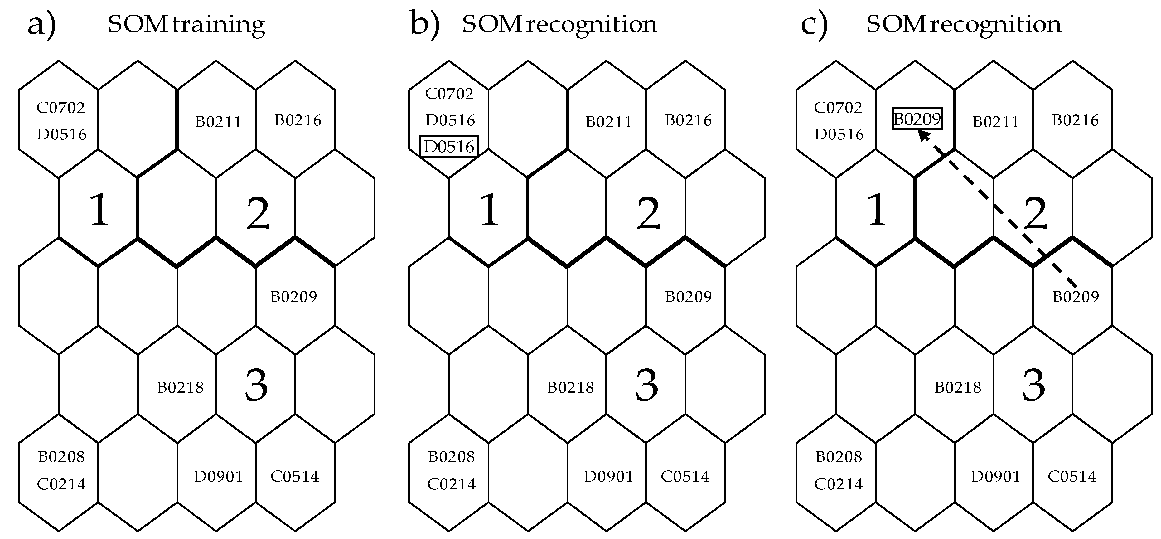
• SOM is trained with the AFLP data and the trained SOM output units are classified to clusters (I, II, …, N) (see Section 2.2).
• A vector, B (list of clusters with training data for each individual) is produced (e.g., B = (I, II, I, III) with the first, second, third, and fourth individual matching cluster I, II, I, and III, respectively). Euclidian distance is calculated between clusters.
• Each locus is altered by flipping over (switching either “presence to absence” or “absence to presence”) separately for each individual.
• Sensitivity analysis is conducted with altered datasets through recognition (See Figure A1).
• A vector, G (list of clusters with altered data) is produced (e.g., G = (I, II, I, I) with each individual sequentially belonging to I, II, I, and I, similar to the case of B in process 2).
• Mean cluster distance for each locus (D) is defined to determine the overall differences between training and recognition for individuals. D is calculated as average of the summed Euclidian distance according to B compared with G. If the change crossed over clusters with higher distance, higher values of distance would be given to this individual.
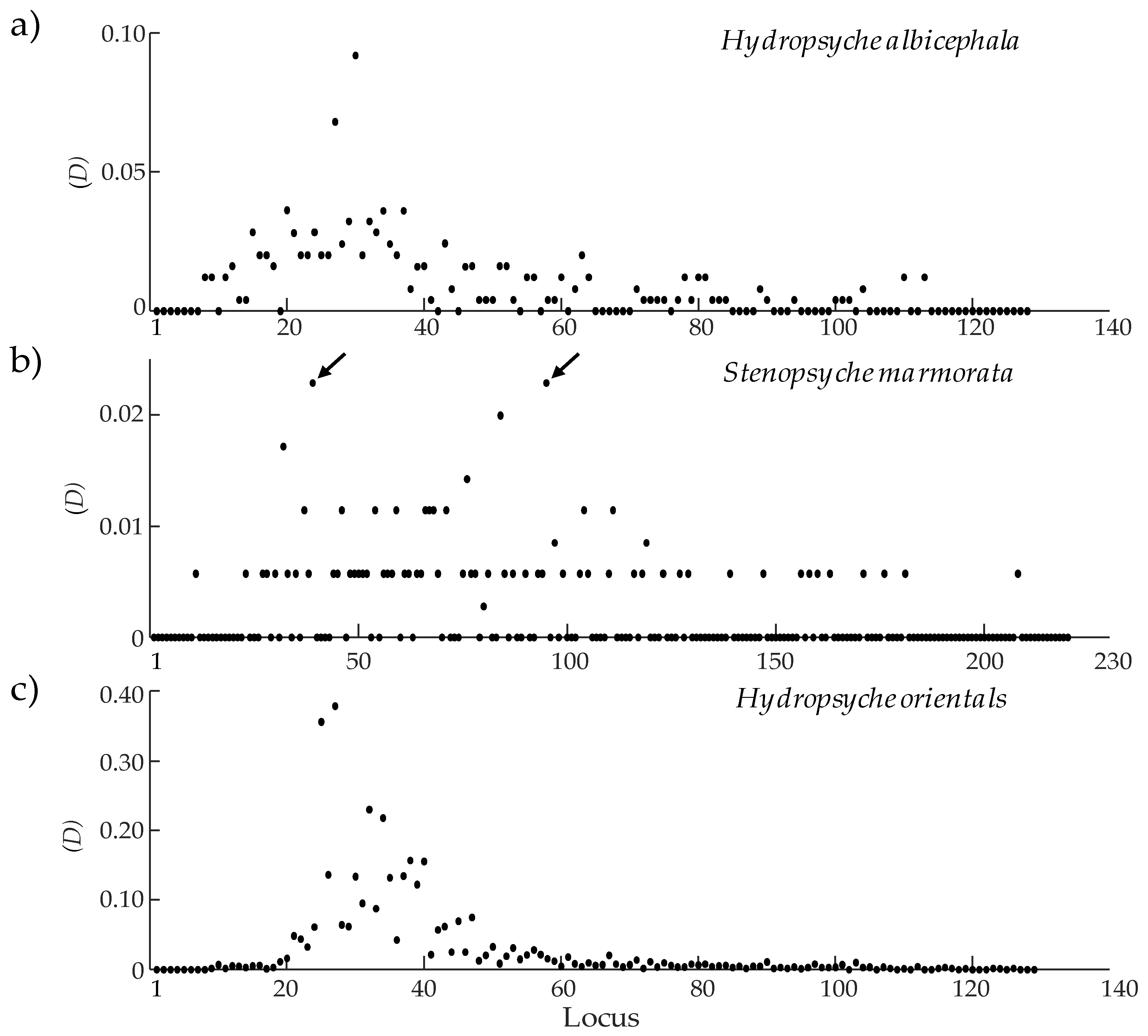
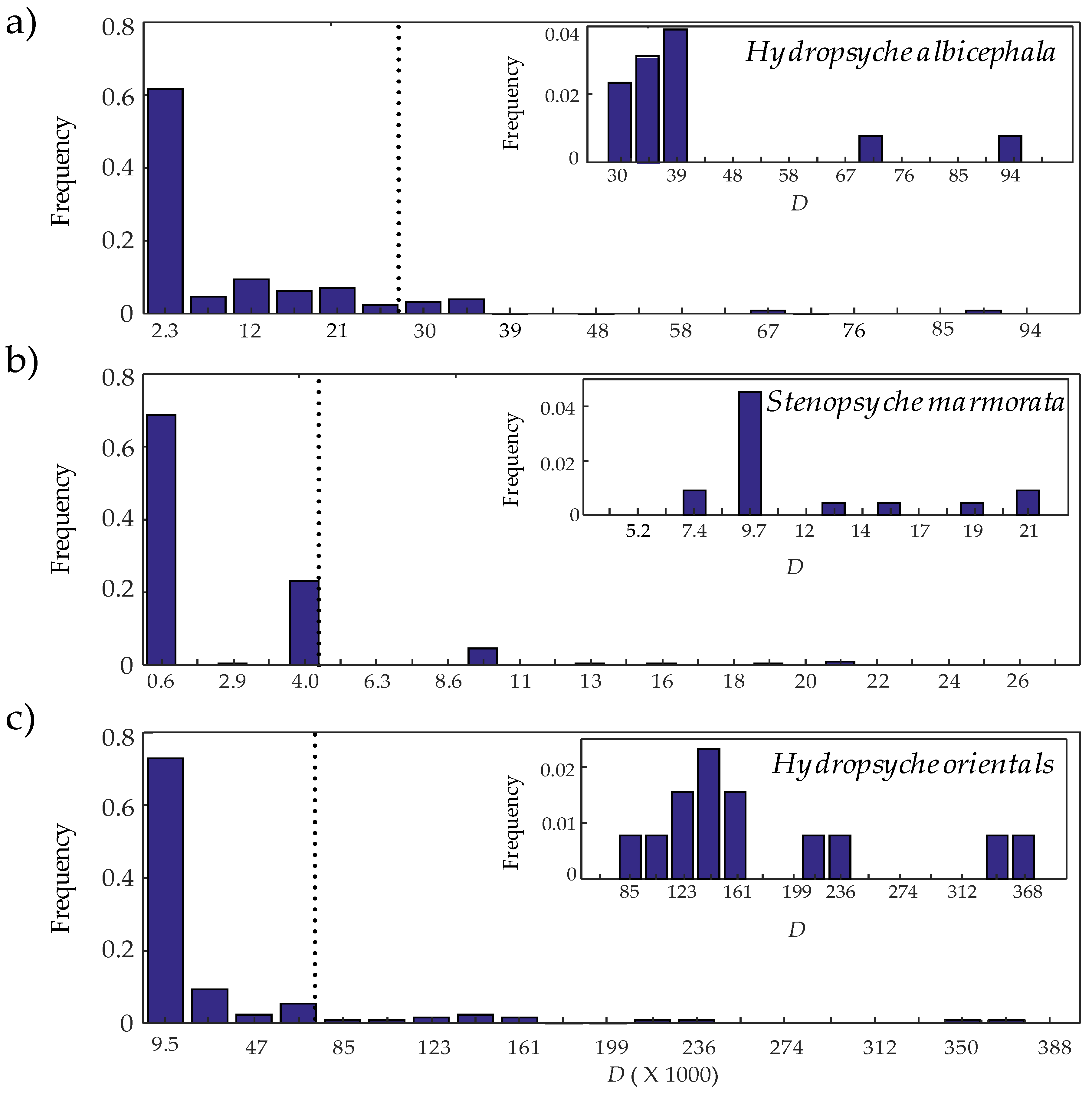
• According to D outlier loci are determined. Loci with D value higher than the 90th percentile [40] were considered as outliers under selection in this study.
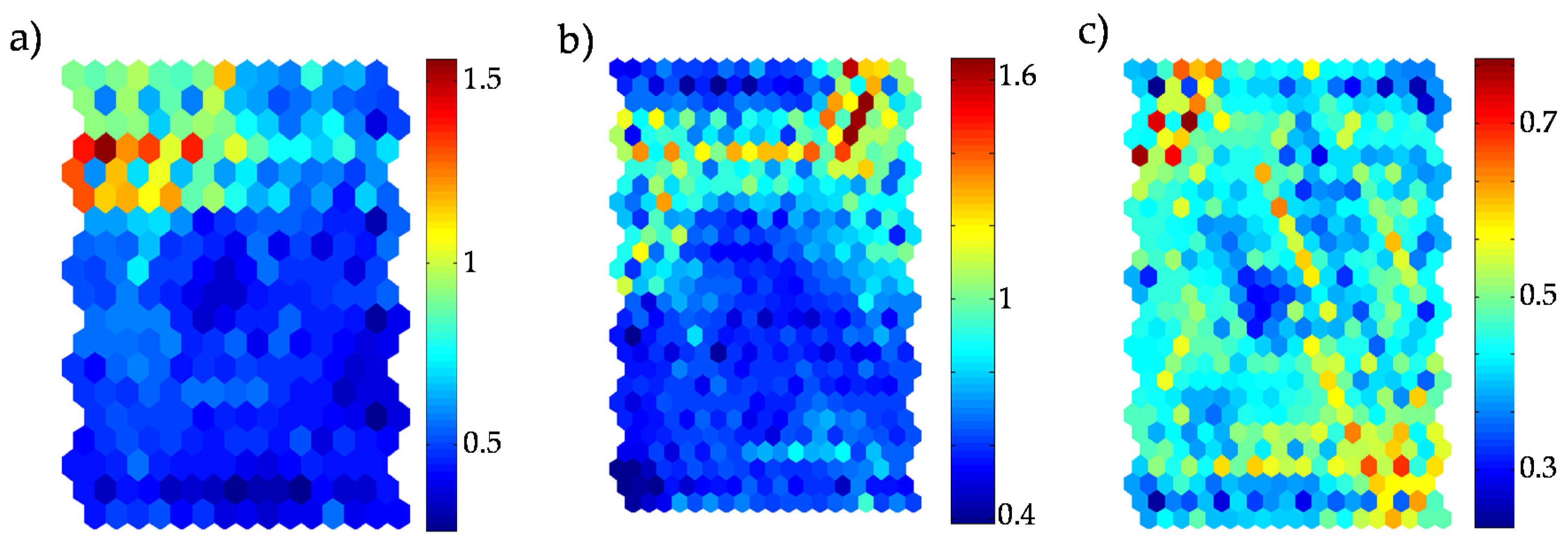
• Once outlier loci were identified, we examined their relationships with each environmental variable. Indices E_k,i and E_k were devised to present responsiveness of each environmental variable (k) in each cluster (i) and overall responsiveness across clusters, respectively, after SOM recognition as follows:

  $$E_{k,i}=|\frac{e_{k,i}-h_{k,i}}{e_{k,i}}|$$

  (1)

  $$E_k=\frac{1}{N}{{\displaystyle \sum }}_1^N{E}_{k,i},$$

  (2)

  where e_k,i is the mean of environmental variable k for all individuals belonging to cluster i before data alteration, h_k,i is the mean of the same environmental variable k for all individuals belonging to cluster i after recognition, and N is the total number of clusters. Higher E_k,i value indicates a higher potential of variation in specific environmental factor, k, due to loci alteration between training and recognition in cluster i, whereas a higher E_k value represents overall responsiveness across all clusters on the SOM.

Take B = (I, II, I, III) and G = (I, II, I, I) in Figure 2 for the case of altitude matching to a certain locus as an example. In B, two individuals belonged to cluster I, corresponding with two values of altitude (100 m and 150 m). Subsequently, the average value was expressed as e_k,i (=125 m). In G, cluster I has three individuals (corresponding with altitudes of 100 m, 150 m, and 200 m) after recognition, and the average of altitude was calculated as 150 m (h_k,i). In order to check the variability in environmental responsiveness, absolute values were used in this study. In the example case, the ratio of change in the mean altitude (absolute value) was 0.2 (E_k,1) between training and recognition in cluster I according to Equation (1). Similarly, we have E_k,2 and E_k,3 values of 0.0 and 1.0 for cluster II and III, respectively. Subsequently the E_k, value for altitude was calculated as the mean value of the three clusters, or 0.4. This indicates the degree of responsiveness of altitude due to data alteration in the locus as 0.4.

In order to present the relative importance of specific environmental factor to the maximum environmental responsiveness, the E_k value was further normalized as E_k’ in relation to maximum value of E_k across all environmental variables (Figure 9) as shown below:

$$E_k^{’}=\frac{E_k}{\max \left(E_k\right)}$$

(3)

Suppose that there are only two environmental variables, altitude and Chl-a with E_k values of 0.4 and 0.8, respectively, for example. Then E_k’ for altitude would be 0.5 whereas E_k’ for Chl-a would be 1.0.

9.

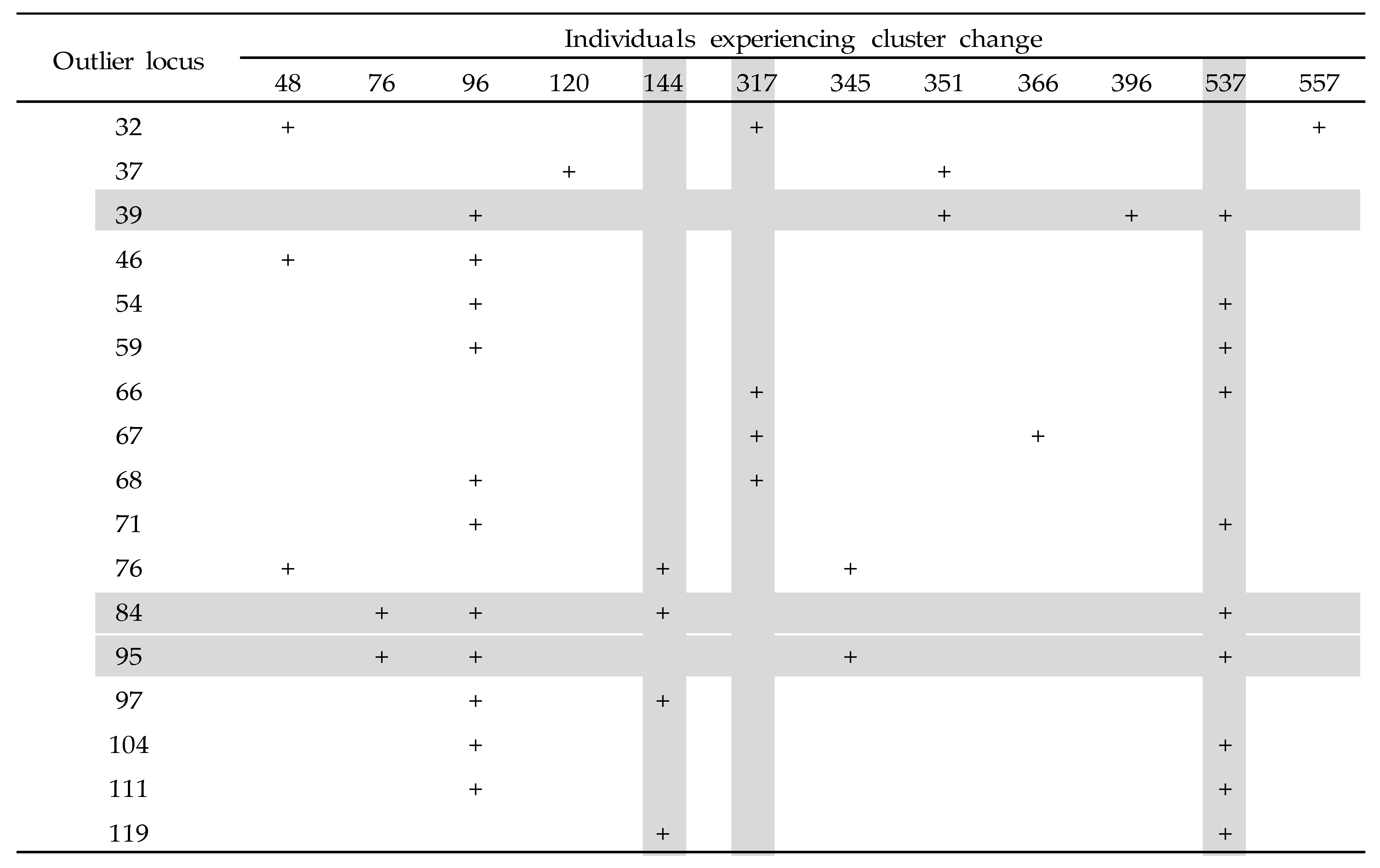
Based on outliers according to D (process 7), a locus-specific pattern showing degree of associations between outlier loci and environmental factors was determined according to the level of E_k’ (process 8) (see Figure 9 for details).

The obtained environmental factors corresponding to outlier loci were cross-checked with the Kolmogorov-Smirnoff test (K-S test) to see whether environmental variables were indeed different across sampling sites [41,42]. In our study, the environmental values were divided into five classes according to different levels. Presence/absence of locus was counted for each individual belonging to the same environmental class and combined to give the overall frequency of loci presence for the individuals collected across different environmental classes. The hypothesis of uniform frequency of loci (i.e., equal presence of loci in different environmental classes) was tested according to the K-S test. For comparing outlier loci, two conventional analyses, the Dfdist and BayeScan methods, were additionally conducted with the same datasets according to Watanabe et al. [8].

3. Results

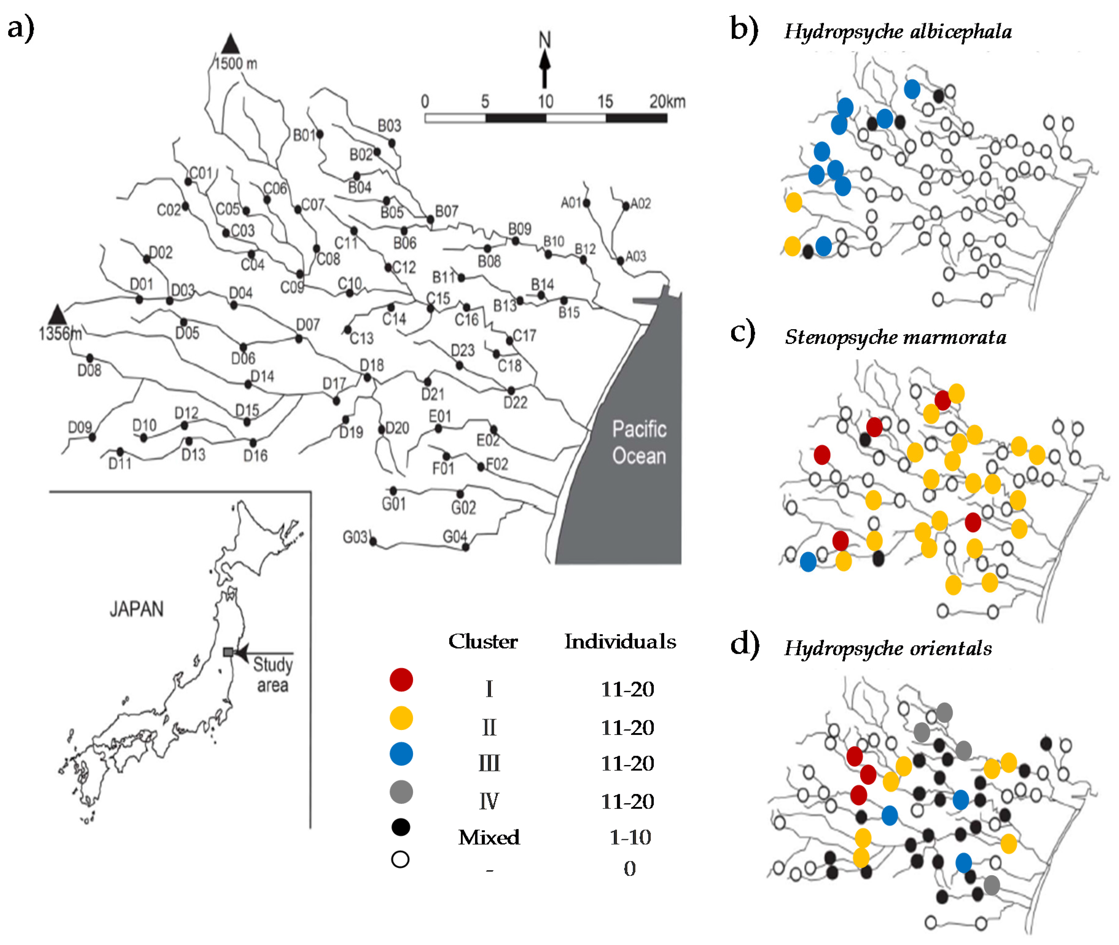
3.1. Habitat Specialization

Based on the SOM trained with nine natural environmental variables (57 sample sites in six streams), grouping was observed according to cluster analysis (Ward linkage method) (Figure 3a). Five clusters were formed based on the dendrogram. Clusters 1, 3, and 4 were observed at the upper area, corresponding with somewhat higher levels in altitude, sediment, BCPOM, and SFPOM according to profiles on the component plane (Figure 3c). Clusters 2 and 5 were placed at the lower area matching higher levels of order, width, mean gravel size, and SFPOM. However, the degree of matching varied according to clusters and environmental variables in both upper and lower groups. For instance, SFPOM was high in both upper and lower groups (Figure 3c). The sampling sites appeared to be mixed in all clusters (Figure 3b). There seemed to be no major environmental factors in determining the overall gradients at the surveyed area according to a visualization of the component profiles (Figure 3c). Habitats are variably characterized by heterogeneous environmental conditions at the sampling sites.

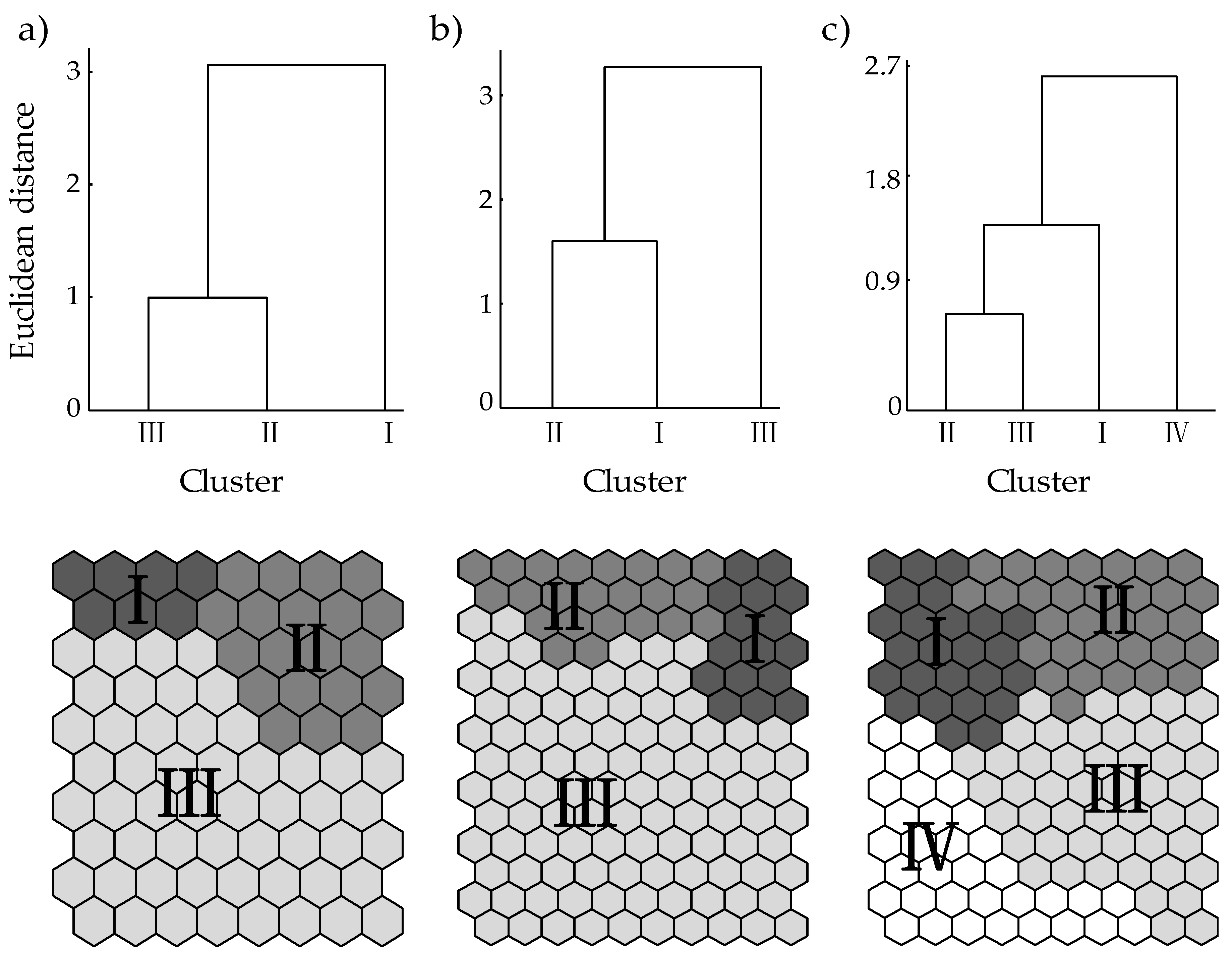
3.2. Patterning of Loci Data

Loci presence/absence data for all individuals were additionally trained with the SOM in each species (see Section 2.2). The number of clusters was determined according to conformation patterns on the U-matrix as shown in Figure A2. Three clusters were chosen for H. albicephela and S. marmorata (Figure 4a,b). In H. orientalis, however, diverse grouping was observed in the U-matrix (Figure A2). After initial training with various numbers of clusters in preliminary studies, four clusters were chosen for grouping the sample units since further division into more clusters did not provide feasible information in characterizing overall loci composition patterns in H. orientalis in this study (Figure 4c).

For the sake of convenience, I was assigned for the most strongly grouped cluster according to the U-Matrix (Figure A2, Figure 4), and the numbers II, III, and IV were subsequently given to the remaining clusters based on the Euclidean distance from cluster II, in ascending order. Clusters I and II occupied a small area and were strongly separated from clusters III and IV, which, by contrast, spanned over a broad area on the SOM (bottom panels, Figure 4).

Figure 1 additionally shows the degree of grouping in different clusters in each site for each species according to the SOM training in Figure 4. The size of solid circles indicates the groups of individuals within the same sampling site (the total number in one site was 20 individuals) in each cluster. The group size of individuals varied according to species. Overall, H. albicephela (Figure 1b) was collected in narrow upstream areas whereas S. marmorata (Figure 1c) and H. orientalis (Figure 1d) were broadly presented over the surveyed streams. In S. marmorata, the large groups (≥ 11 individuals) mostly belonged to intermediately (II) and strongly (I) grouped clusters (Figure 1c). The large groups were similarly found at the intermediately grouped cluster II in H. orientalis (Figure 1d). However, large groups were also found in all other clusters to a somewhat lesser degree in this species. It was also noteworthy that small groups (≤ 10 individuals) without dominant clusters were abundantly observed in H. orientalis. In H. albicephela, which was narrowly distributed upstream only, large groups were mainly observed in the weakly grouped cluster III (Figure 1b).

3.3. Identifying Outlier Loci and Environmental Responsiveness

The importance of variables (i.e., loci) was checked by recognizing the altered data with the trained SOM in a similar sensitivity test (see Section 2.3 and Processes 3–9 in Figure 2). Cluster distances according to presence of loci (i.e., higher presence, higher rank on x axis) are presented in Figure 5. The patterns of distance distribution varied according to species. The D values were variably observed in H. albicephela and H. orientalis (Figure 5a,c). The highest range, including peaks, was commonly observed at the ranks of 20–35 for both species. In S. marmorata, however, we found several fixed values of D, including 0.006 and 0.011 (Figure 5b). This indicated that a fixed number of individuals were commonly selected to experience cluster changes in this species. It was noteworthy that the two loci with the maximum D value (0.023) in S. marmorata were observed at loci 39 and 95, respectively (arrows in Figure 5b).

Profiles of cluster distance are presented according to the order of D values, from low to high, in each species (Figure 6). Although SOMs could not be directly compared between species due to the separate SOM trainings for each species (see Section 2.2), overall trends and conformation of D values were separable and characteristic according to species. Usually a sharp drop of D was observed immediately after the peak by one or two-top ranked loci (Figure 6). The maximum D value (0.378) was observed in H. orientalis (Figure 6c), whereas S. marmorata had the minimum value (0.023) for the top rank locus (Figure 6b). Ranges in the number of individuals experiencing cluster changes (the gray shades in Figure 6) varied, with 0%–7.6%, 0%–0.7%, and 0%–21.5% for H. albicephela, S. marmorata, and H. orientalis, respectively. S. marmorata had the minimum proportion of individuals experiencing cluster changes, whereas the total number of individuals (571) used for training was intermediate compared with H. albicephela (251) and H. orientalis (753). Cluster change patterns were overall similar in the three species in accordance with the rank of loci, decreasing as the rank decreased (Figure 6).

When frequencies were presented across different levels of D in the histogram, the maximum value was observed with the minimum level of D in different species (Figure 7). Frequencies sharply decreased in all species as D increased along the x axis. According to the frequency distribution shown in Figure 7, the outlier loci that responded strongly to data alteration were identified. In order to determine outliers, the 90th percentile was set as the threshold for each species (vertical lines in Figure 7) (see Section 2.3); the loci showing higher levels of D than the threshold were chosen as outlier loci in this study. Since many individuals showed the same value of D at the boundary of the 90th percentile line for S. marmorata, the grouped individuals that crossed the boundary of the percentile line were not included as outliers for S. marmorata. The numbers of outlier loci were 14, 17, and 12 for H. albicephela, S. marmorata, and H. orientalis, respectively (

Table 2. Similarity indices and number of common outliers between Dfdist, BayeScan, and SOM.

Species	No. of Outlier Loci				Dfdist vs. BayeScan		Dfdist vs. SOM		BayeScan vs. SOM
	BayeScan	Dfdist	SOM	Common Outliers	Similarity Index	No. of Common Outliers	Similarity Index	No. of Common Outliers	Similarity Index	No. of Common Outliers
Hydropsyche albicephala	16	7	14	3	0.35	6	0.17	3	0.2	5
Stenopsyche marmorata	56	23	17	10	0.36	21	0.34	10	0.28	16
Hydropsyche orientals	31	9	12	4	0.29	9	0.22	4	0.16	6

), and the outlier loci were listed in

Table A1. List of outlier loci identified by Dfdist, BayeScan, and SOM.

Species	Dfdist vs. BayeScan	Dfdist vs. SOM	BayeScan vs. SOM	Common Outliers
Hydropsyche albicephala	4, 5, 11, 15, 29, 43	15, 29, 43	15, 29, 33, 35, 43	15, 29, 43
Stenopsyche marmorata	32, 33, 34, 43, 45, 56, 66, 67, 68, 70, 76, 78, 80, 84, 85, 95, 97, 104, 106, 111, 116	32, 66, 67,68, 76,84, 95, 97, 104, 111	32, 37, 39, 46, 54, 59, 66, 67, 68, 71, 76, 84, 95, 97, 104, 111	32, 66, 67, 68, 76, 84, 95, 97, 104, 111
Hydropsyche orientals	20, 25, 27, 39, 40, 47, 49, 53, 67	25, 27, 39, 40	25, 26, 27, 32, 39, 40	25, 27, 39, 40

.

Subsequently we checked what clusters on the SOM responded to data alteration more sensitively. Figure 8 shows how clusters were affected when cluster change occurred for individuals in each species after SOM recognition (see Section 2.3). The cluster difference was evaluated according to the Jaccard similarity index [43] (J = c/(a + b − c), where c is the commonly found individuals and a and b are the total number of individuals found in the cluster before and after recognition, respectively). Subsequently the value of F = 1 − J was used to represent cluster difference. For convenience of visualization, all values were normalized to 0 to 1 based on the maximum F value obtained for each species, as shown by the vertical bars in Figure 8. The patterns of cluster change were different according to species. In H. albicephela, cluster II followed by cluster I were mainly affected by the altered data (Figure 8a). One locus in cluster II (locus 35) showed an especially high level of cluster difference. S. marmorata similarly showed a stronger response in clusters I and II (Figure 8b). In this case cluster I presented the highest level of F in selected loci (e.g., loci 71, 97, and 111). In H. orientalis, by contrast, cluster II and the weakly grouped clusters IV and III were more affected by the altered data (Figure 8c). The overall results indicated that sensitivity in loci composition varied according to different species.

By calculating environmental responsiveness E_k‘ (Equation (3), see Section 2.3), each environmental factor was presented to associate specifically with outlier loci (Figure 9). For convenience of visualization, all E_k‘ values were normalized in the range of 0.00–1.00 based on the maximum E_k value across environmental variables in each species, as stated above (vertical bars, Figure 9). Maximum E_k values were found with Chl-a (1.28), NH₄-N (0.76), and Chl-a (0.22) for species H. albicephela, S. marmorata, and H. orientalis respectively. E_k values were relatively small for H. orientalis although the proportion of individuals experiencing cluster change was high (Figure 6c). The environmental responsiveness was characteristically observed according to species. In H. albicephela, Chl-a (0.94–1.00) showed outstandingly high E values, followed by epilithon (0.43–0.44) (Figure 9a). H. orientalis similarly showed the highest responsiveness to Chl-a (0.75–1.00) and epilithon (0.64–0.72). In addition, PO₄-P (0.56–0.67), NO_X–N (0.54–0.56), and altitude (0.43–0.60) presented higher values in this species (Figure 9c). S. marmorata was characteristically sensitive to various anthropogenic stresses of NH₄–N (0.97–1.00), followed by PO₄–P (0.45–0.46), SS (0.32–0.33), and somewhat to sediment (0.24–0.25) (Figure 9b). Species overall responded highly to various anthropogenic factors and epilithon, and to a lower degree to natural factors (i.e., altitude and sediment).

Two points can be summarized in terms of environment-outlier relationships. First, many loci were concurrently involved in responding to specific environmental factors, suggesting poly-loci-like responsiveness to environmental constraints (Figure 9). Secondly, outliers were mainly sensitive to either pollution agents (e.g., Chl-a, NH₄–N, NO_X–N, PO₄–P, and SS) or feeding material (i.e., epilithon).

We further checked whether the results from SOM sensitivity would be in accordance with the difference in environmental factors measured at different sampling sites. A K-S test was conducted to check the significant difference between different levels of environmental variables (see Section 2.3). With all the environmental variables, the significance was only observed at p < 0.05 without a lower level of alpha error (e.g., p < 0.01). The symbol “*” was superimposed on the cells (presenting each combination of locus and environmental variable) shown in Figure 9. Significance in the K-S test corresponded with a high overall environmental responsiveness, indicating that the sensitivity in loci was in accordance with differences in environmental variables. There were some mismatches, however. PO₄–P in S. marmorata and H. orientalis, for instance, did not show overall significance in the K-S test, although the environmental responsiveness was high (Figure 9b,c).

It was noteworthy that the maximum values of pollution at the sampling sites were not indicative of severe conditions but rather indicated a low degree of pollution (

Table 3. Summary of water quality indicators measured at sampling sites (n = 57) compared with WHO standards. (Minimum value of suspended solid is not recorded in WHO standards). For Chl-a, the number of significant digits is four for precise measurement.

Variables	Unit	Mean ± SD	Observed Values		WHO Standards a		Comparison (%) b
			Minimum	Maximum	Minimum	Maximum
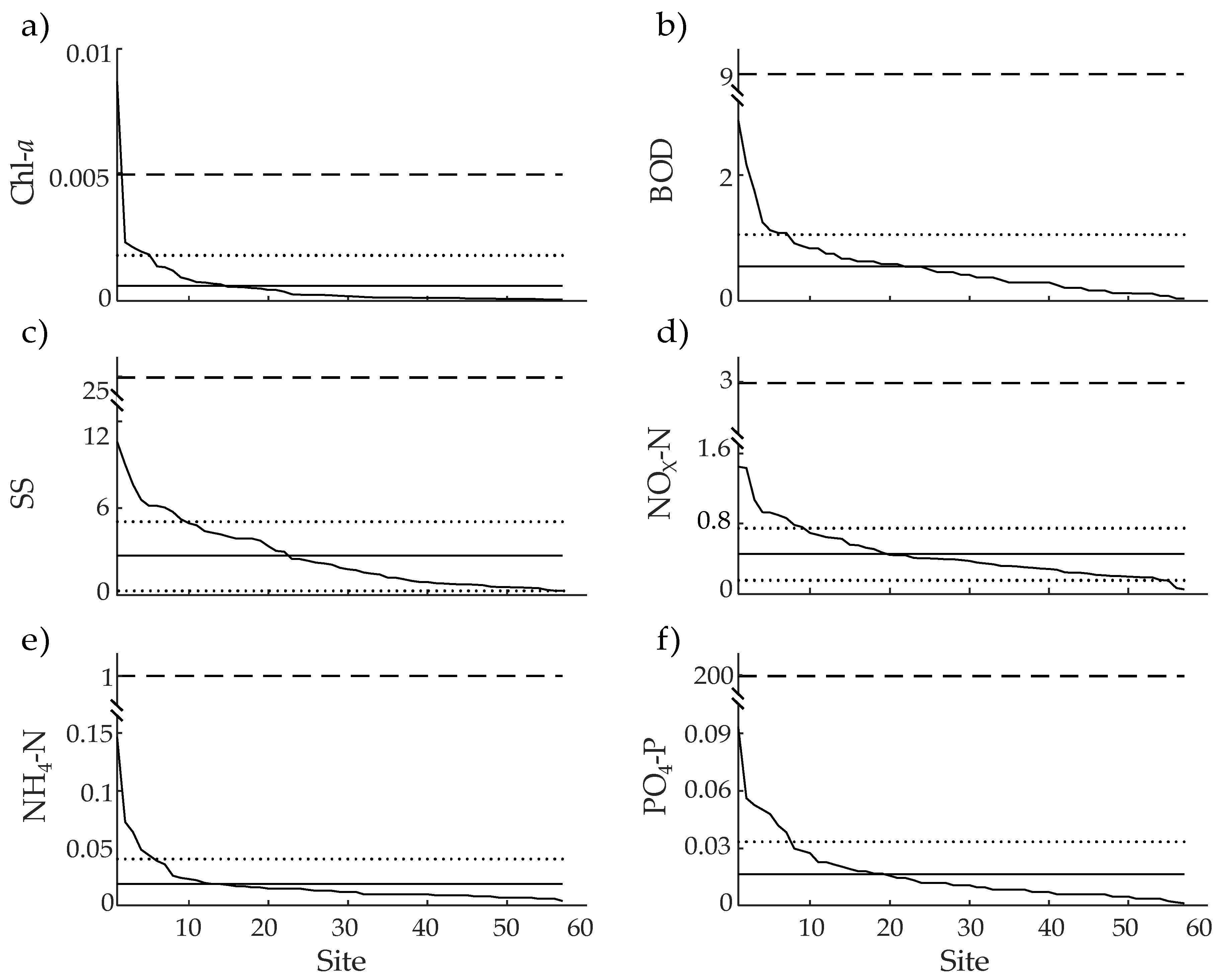
Chl-a	mg·L−1	0.000,6 ± 0.001,2	0.0001	0.0087	<0.0025	0.005,0–0.140,0 c	12.000,0
BOD	mg·L−1	0.455 ± 0.430	0.035	2.394	2 or less than 2	9	5.057
SS	mg·L−1	3.004 ± 2.653	0.318	11.756	–	25	12.016
NOX–N	mg·L−1	0.475 ± 0.313	0.055	1.513	<0.1	3	15.817
NH4–N	mg·L−1	0.019 ± 0.022	0.004	0.147	0.04	1	1.880
PO4–P	mg·L−1	0.013,4 ± 0.014	0.001	0.078	0.001	200	0.007

^a: Significant digits are based on the original data; ^b: Mean of observed value divided by maximum value (WHO standards); ^c: Maximum concentration of Chl-a was chosen as 0.0050 mg·L⁻¹ instead of 0.1400 mg·L⁻¹.

). The gradients of water quality indicators across all the sampling sites are presented in Figure A3. According to WHO standards [44], water quality indicators measured in this study were substantially low. When the average values of the observed data were compared with the maximum level in the WHO standards, PO₄–P and NH₄–N showed the minimal range with 0.007%–1.880%. BOD had a somewhat higher level of 5.057% whereas NOx–N, SS, and Chl-a presented maximal levels of 15.817%, 12.016%, and 12.000%, respectively (Table 3). All observed measurements in this study, however, were substantially low compared with the WHO standards.

The outliers detected by SOM, Dfdist [15], and BayeScan [18] are compared in Table 2. Since the number of detected outliers varied according to different methods, similarity in outliers between different methods was measured by the Jaccard similarity index [43] (J = c/(a+b–c), where c is the commonly detected loci and a and b are the total number of detected loci by each method, respectively). Between Dfdist and BayeScan, the indices were in the range of 0.18–0.36 for all species (Table 2). Indices of SOM in relation to Dfdist and BayeScan were in a comparable range, 0.16–0.34. Among the three species, S. marmorata showed the highest number of outliers with 17, 56, and 23 loci for SOM, BayeScan, and Dfdist, respectively (Table 2, Table A1). A substantial number of common loci between different methods were also observed in S. marmorata: 21 in Dfdist vs. BayeScan, followed by 16 in BayeScan vs. SOM, and 10 in Dfdist vs. SOM. In the other two species the number of common loci between different methods was in the range 3–9 (Table 2).

4. Discussion

The current study demonstrated that specific associations between outlier loci and environmental variables could be effectively mined based on SOM even though a priori knowledge regarding population genetics (e.g., coalescent theory) is not available. Complexity residing in the presence/absence of loci was effectively extracted when they were exposed to complex effects of environmental factors according to different sampling sites. Whereas conventional methods such as Dfdist and BayeScan are mainly based on population genetics theories and statistical parameters (e.g., correlation coefficient between Wright’s fixation index (F_ST) and environmental variables) [8,45,46], the SOM approach reveals relationships between outlier loci and environmental variables through information processing (Figure 4, Figure 5, Figure 6, Figure 7, Figure 8 and Figure 9). The topology of complex data structure in multiple dimensions was effectively preserved in a reduced dimension through a self-organizing process [24]. It was noteworthy that environmental variables were specifically identified in association with each outlier based on the SOM approach de novo (Figure 9).

Loci were responsive to anthropogenic environmental change although the pollution level was low at the sampling sites (Figure 9, Table 3, and Figure A3). Based on the conventional methods (Dfdist and BayeScan), Watanabe et al. [8] reported that differences in F_ST at non-neutral loci were strongly related with natural and anthropogenic sources of Chl-a in H. albicephela, BCPOM in S. marmorata, and altitude in both S. marmorata and H. orientalis. A somewhat weak response was observed with velocity, epilithon, and NH₄–N in H. orientalis. This study partly confirmed results by Watanabe et al. [8] including Chl-a in H. albicephela, and altitude and epilithon in H. orientalis. However, overall differences were also observed. Response to anthropogenic stress appeared to be more prevalent in this study. H. orientalis showed high responsiveness to Chl-a in addition to H. albicephela (Figure 9c). S. marmorata additionally showed diverse responsiveness to NH₄–N, followed by PO₄–P and SS (Figure 9b). It was noteworthy that BOD showed generally lower levels of environmental responsiveness than other indicators in this study, except in H. orientalis (E_k’ ranging from 0.31 to 0.44) (Figure 9c). Response to natural environmental factors, however, was not strongly observed except for the feeding material, epilithon, followed by altitude and sediment to a lesser degree, as stated above. Future study is warranted in revealing these loci-environment relationships in natural and anthropogenic variability more precisely along with gene functioning and physiological network studies.

Although overall trends were in accordance between the environmental response and the K-S results, there were discrepancies between the two tests (Figure 9). Whereas the K-S test only reveals statistical differences in environmental factors separately (i.e., factor by factor), SOM deals with all variables together, accommodating complex interrelationships among variables concurrently in a non-linear manner through information processing. For instance, PO₄-P values were significantly different according to the K-S test in S. marmorata and H. orientalis, although the E_k‘ values were substantially lower (Figure 9). However, the detailed mechanism whereby environmental responsiveness was specifically sensitive to outlier loci is unknown. More studies regarding genetic functioning and molecular ecology are needed in the future.

Clusters with a small number of individuals (≤ 10 individuals) were characteristically found in H. orientalis (Figure 1d). In S. marmorata, however, not many small groups were found and large groups of individuals were observed mainly in the intermediately grouped cluster II (Figure 1c). Following cluster II, more large individual groups were additionally found in the strongly grouped cluster I than in the weakly grouped cluster III in this species. In H. albicephela, by contrast, a large number of individuals were mainly observed in cluster III (Figure 1b). This indicated that loci composition patterns varied according to species. The somewhat more closely related loci (i.e., being more different from other clusters according to SOM) observed in S. marmorata, for instance, had a stronger susceptibility to selection pressure, and consequently a higher potential for cluster change in more strongly grouped clusters. In H. albicephela, by contrast, the selection pressure may be not strong enough to cause loci variability in the strongly grouped clusters.

Difference in cluster change (F) also reflected the group responses of individuals. For instance, the intermediately and strongly grouped clusters I and II were particularly affected in S. marmorata (Figure 8b); large groups of individuals experiencing cluster changes were found in these clusters (Figure 1c). In H. orientalis, by contrast, the cluster change effect was mainly observed in the intermediately and weakly grouped clusters II, III, and IV, whereas a minimum response was observed in the strongly grouped cluster I (Figure 1d and Figure 8c).

The loci composition patterns according to the SOM may match the dispersal ability of a species. It was reported that dispersal potential is weak for H. orientalis, whereas it is intermediate for S. marmorata according to Watanabe et al. [47]. The patterns of individual groupings were different between the two species. Whereas the intermediately and strongly grouped clusters II and I had large groups of individuals for cluster change at the same sampling sites in S. marmorata (Figure 1c), the small-group individuals (≤ 10 individuals) within one cluster (i.e., without dominating clusters) were mainly observed for cluster change in H. orientalis (Figure 1d), as stated above. This indicated that loci information is more fractional (i.e., there is a higher chance of variation in loosely grouped loci) in species like H. orientalis with low dispersal potential. However, in S. marmorata, which has intermediate dispersal potential, selection pressure would more strongly occur in strongly-grouped loci compositions (Figure 1c). However, drawing any conclusion regarding the relationships between dispersal ability and genetic divergence is still premature; additional studies on molecular ecology and gene functioning are needed in this regard in the future.

Specific individuals causing cluster changes could also be identified. We checked the fixed levels of D observed in S. marmorata (Figure 5b). The discrete values shown in S. marmorata were due to specific individuals changing consistently across different loci either in groups or as individuals. Initially S. marmorata showed individuals experiencing cluster changes separately. For example, individual 96 experienced cluster changes in numerous loci including 11, 23, 27, 44, etc., while individual 537 separately experienced cluster changes in loci including 30, 45, 49, 64, etc. (Figure A4). In addition, certain individuals (e.g., (48, 317, 557), (96, 537)) contributed to cluster changes together. Since a fixed number of individuals showed cluster changes, this was the reason why these species showed discreteness in D (Figure 5b). Two peaks were additionally observed in D values in relation to the frequency of loci presence in S. marmorata (arrows in Figure 5b). The reason for obtaining two peaks in this species is currently unavailable. The strong responsiveness may be due to different types of data alteration (e.g., difference in “presence to absence” and “absence to presence” of loci), but close examination is required regarding input–output data relationships and genetic/ecological functioning.

In this study binary values were used as input (presence/absence). If continuous variables are used as input data, a small amount of noise could be added to cause continuous variability in the input data over a small range, similar to a conventional sensitivity analysis. However, the binary values were changed totally (either “1 to 0” or “0 to 1”) in this study for training and recognition. Subsequently recognition was conducted to address the local effect of data alteration; the cluster change due to an altered datum for each locus was examined for each individual on the trained map (see Section 2.3).

In Paini et al. [34] binary data (presence or absence of pest species in different regions) were similarly used for training pest occurrence in different sampling sites. A different number of species (variables) was selected for data alteration (flipping over) according to different proportion levels (0.05, 0.10, 0.20, and 0.30). Subsequently the SOM was newly generated after data alteration. The variability of SOM output due to retraining was used as a criterion to determine stability in risk assessment. Data alteration of 0.30 indicated significant changes compared to original groupings whereas 0.20 indicated stability in groupings. The sensitivity test performed by Paini et al. [34] was useful for confirming the robustness of our predictions of pest invasion risk.

In our study, however, we focused on investigating the specific contribution of each locus (variable) on the cluster patterns. We adopted a recognition process after training (Figure 2). By examining the result of recognition on the trained SOM locally, the patterns of cluster change were specifically observed locus by locus for each individual (Figure A1). Further associations between loci and environmental variable were revealed according to this type of SOM training followed by recognition (Figure 9). However, variability would still be obtained in initial training if random conditions were different in different trials. Since convergence is obtained adaptively through a random process, as stated above, a minor degree of variability would exist in either clustering or determining outliers, although the overall trends would be similar. Further research is required to optimize the variability caused by randomness in SOM training in relationship with outlier determination in the future.

Considering flexibility in data handling and information extraction processes, SOM could be extended to link with the models used in conventional methods based on population genetics. Either a hybrid model or SOM network modification could be considered for addressing the interplay between information processing and molecular ecology. In addition, SOM could be further applied to diverse taxa and experimental data related to ecological (e.g., functional feeding group) and genetic functioning.

5. Conclusions

Addressing ecological functioning garners special attention in association with aquatic ecosystem management since the status of live organisms in ecosystems would reveal the direct effects of water quality. SOM was effective in addressing relationships between loci and environmental factors through training and recognition, although specific gene information and/or population genetics (e.g., coalescent theory) are not available for loci data. By applying the SOMs to AFLP of aquatic insects collected in six streams in Japan, we proved that the genetic information of aquatic insects responds sensitively to anthropogenic and natural selection pressures. Outlier loci over the 90th percentile were associated with environmental factors pertaining to specific sampling sites and were comparable with the conventional methods (Dfdist and BayeScan). Some loci were sensitive to pollutants at low levels including Chl-a, NH₄–N, NO_X–N, PO₄–P, and SS. The feeding material, epilithon, also served as a source of selection pressure. Loci compositions further responded to natural factors including altitude and sediment, but to a lesser degree. In addition, poly-loci-like responsiveness was detected in respond to environmental constraints.

Gene information adapting to environmental stress would be accordingly reflected in information processing. SOM training combined with recognition shed a light on developing algorithms de novo to characterize loci without a priori knowledge of population genetics used for conventional methods. For further understanding of genetic diversity in adapting to environmental constraints, more studies are warranted on both informatics (e.g., the development of networks) and biological (e.g., ecological/genetic functioning) aspects in the future.

References

- Allan, J.D. Landscapes and riverscapes: The influence of land use on stream ecosystems. Annu. Rev. Ecol. Evol. Syst. 2004, 35, 257–284. [Google Scholar] [CrossRef]
- Walsh, C.J.; Roy, A.H.; Feminella, J.W.; Cottingham, P.D.; Groffman, P.M.; Morgan, R.P. The urban stream syndrome: Current knowledge and the search for a cure. J. North Am. Benthol. Soc. 2005, 3, 706–723. [Google Scholar] [CrossRef]
- Hellawell, J.M. Biological indicators. In Biological Indicators of Freshwater Pollution and Environmental Management, 1st ed.; Hellawell, J.M., Ed.; Elsevier Science Publishing Co., Inc: New York, NY, USA, 1986; pp. 45–63. [Google Scholar]
- Rosenberg, D.M.; Resh, V.H. Introduction to Freshwater Biomonitoring and Benthic Macroinvertebrates. In FreshwaterBiomonitoring and Benthic Macroinvertebrates, 1st ed.; Rosenberg, D.M., Resh, V.H., Eds.; Chapman & Hall: New York, NY, USA, 1993; pp. 1–30. [Google Scholar]
- Wright, J.F. An introduction to RIVPACS. In Assessing the Biological Quality of Freshwaters, RIVPACS and Other Techniques; Wright, J.F., David, W.S., Mike, T.F., Eds.; Freshwater Biological Association: Ambleside, UK, 2000; pp. 5–26. [Google Scholar]
- Park, Y.S.; Song, M.Y.; Park, Y.C.; Oh, K.H.; Cho, E.C.; Chon, T.S. Community patterns of benthic macroinvertebrates collected on the national scale in Korea. Ecol. Model. 2007, 203, 26–33. [Google Scholar] [CrossRef]
- Storz, J.F. Invited Review: Using genome scans of DNA polymorphism to infer adaptive population divergence. Mol. Ecol. 2005, 14, 671–688. [Google Scholar] [CrossRef] [PubMed]
- Watanabe, K.; Kazama, S.; Omura, T.; Michael, T.M. Adaptive Genetic Divergence along Narrow Environmental Gradients in Four Stream Insects. PLoS ONE 2014, 9, e93055. [Google Scholar] [CrossRef] [PubMed]
- Kim, J.; Lee, T. An integrated approach of comparative genomics and heritability analysis of pig and human on obesity trait: Evidence for candidate genes on human chromosome 2. BMC Genom. 2012, 13, 711. [Google Scholar] [CrossRef] [PubMed]
- Tabor, H.K.; Risch, N.J.; Myers, R.M. Candidate-gene approaches for studying complex genetic traits: Practical considerations. Nat. Rev. Genet. 2002, 3, 391–397. [Google Scholar] [CrossRef] [PubMed]
- Carneiro, M.; Afonso, S.; Geraldes, A.; Garreau, H.; Bolet, G.; Boucher, S.; Tircazes, A.; Queney, G.; Nachman, M.W.; Ferrand, N. The genetic structure of domestic rabbits. Mol. Biol. Evol. 2011, 28, 1801–1816. [Google Scholar]
- Daniels, S.E.; Bhattacharrya, S.; James, A.; Leaves, N.I.; Young, A.; Hill, M.R.; Faux, J.A.; Ryan, G.F.; le Souef, P.N.; Lathrop, G.M.; et al. A genome-wide search for quantitative trait loci underlying asthma. Nature 1996, 383, 247–250. [Google Scholar] [CrossRef] [PubMed]
- Verhoeven, K.J.F.; Vanhala, T.K.; Biere, A.; Nevo, E.; van Damme, J.M. The genetic basis of adaptive population differentiation: A quantitative trait locus analysis of fitness traits in two wild barley populations from contrasting habitats. Evolution 2004, 58, 270–283. [Google Scholar] [CrossRef] [PubMed]
- Rogers, S.M.; Bernatchez, L. Integrating QTL mapping and genome scans towards the characterization of candidate loci under parallel selection in the lake whitefish (Coregonus clupeaformis). Mol Ecol. 2005, 14, 351–361. [Google Scholar] [CrossRef] [PubMed]
- Beaumont, M.A.; Nichols, R.A. Evaluating loci for use in the genetic analysis of population structure. Proc. Roy. Soc. B Biol. Sci. 1996, 263, 1619–1626. [Google Scholar] [CrossRef]
- Beaumont, M.A.; Balding, D.J. Identifying adaptive genetic divergence among populations from genome scans. Mol Ecol. 2004, 13, 969–980. [Google Scholar] [CrossRef] [PubMed]
- Foll, M.; Gaggiotti, O.E. Identifying the environmental factors that determine the genetic structure of populations. Genetics 2006, 74, 875–891. [Google Scholar] [CrossRef] [PubMed]
- Foll, M.; Gaggiotti, O.E. Estimating selection with different markers and varying demographic scenarios: A Bayesian perspective. Genetics 2008, 180, 977–993. [Google Scholar] [CrossRef] [PubMed]
- Strachan, T.; Read, A. Genes in Pedigrees and Populations. In Human Molecular Genetics; Garland Science: New York, NY, USA, 2009. [Google Scholar]
- Lotterhos, K.E.; Whitlock, M.C. Evaluation of demographic history and neutral parameterization on the performance of FST outlier tests. Mol. Ecol. 2014, 23, 2178–2192. [Google Scholar] [CrossRef] [PubMed]
- Straškraba, M. Ecotechnological models for reservoir water quality management. Ecol. Model. 1994, 74, 1–38. [Google Scholar] [CrossRef]
- Hamilton, G.; McVinish, R.; Mengersen, K. Bayesian model averaging for harmful algal bloom prediction. Ecol. Appl. 2009, 19, 1805–1814. [Google Scholar] [CrossRef] [PubMed] [Green Version]
- Fornarelli, R.; Galelli, S.; Castelletti, A.; Antenucci, J.P.; Marti, C.L. An empirical modeling approach to predict and understand phytoplankton dynamics in a reservoir affected by interbasin water transfers. Water Resour. Res. 2013, 49, 3626–3641. [Google Scholar] [CrossRef]
- Kohonen, T. The self-organizing map. Proc. IEEE 1990, 78, 1464–1480. [Google Scholar] [CrossRef]
- Park, Y.-S.; Tison, J.; Lek, S.; Coste, M.; Giraudel, J.; Delmas, F. Application of a self-organizing map in ecological informatics: Selection of representative species from large community dataset. Ecol. Inform. 2006, 1, 247–257. [Google Scholar] [CrossRef]
- Chon, T.-S. Self-Organizing Maps applied to ecological sciences. Ecol. Inform. 2011, 6, 50–61. [Google Scholar] [CrossRef] [PubMed]
- Ferrán, E.A.; Ferrara, P. Clustering proteins into families using artificial neural networks. Bioinformatics 1992, 8, 39–44. [Google Scholar]
- Nikkilä, J.; Törönen, P.; Kaski, S.; Venna, J.; Castrén, E.; Wong, G. Analysis and visualization of gene expression data using Self-Organizing Maps. Neural Netw. 2002, 15, 953–966. [Google Scholar] [CrossRef]
- Chavez-Alvarez, R.; Chavoya, A.; Mendez-Vazquez, A. Discovery of Possible Gene Relationships through the Application of Self-Organizing Maps to DNA Microarray Databases. PLoS ONE 2014, 9, e93233. [Google Scholar]
- Giraudel, J.L.; Aurelle, D.; Berrebi, P.; Lek, S. Application of the self-organizing mapping and fuzzy clustering to microsatellite data: How to detect genetic structure in brown trout (Salmo trutta) populations. In Artificial Neuronal Networks; Lek, S., Guégan, J.F., Eds.; Springer: New York, NY, USA, 2000; pp. 187–202. [Google Scholar]
- Kontunen-Soppela, S.; Parviainen, J.; Ruhanen, H.; Brosché, M.; Keinäen, M.; Thakur, R.C.; Kolehmainen, M.; Kangasjävi, J.; Oksanen, E.; Karnosky, D.F.; et al. Gene expression responses of paper birch (Betula papyrifera) to elevated CO2 and O3 during leaf maturation and senescence. Environ. Pollut. 2010, 158, 959–968. [Google Scholar] [CrossRef] [PubMed]
- Cho, S.Z.; Jang, M.; Reggia, J.A. Effects of Varying Parameters on Properties of Self-Organizing Feature Maps. Neural Process. Lett. 1996, 4, 53–59. [Google Scholar] [CrossRef]
- Gonzalez, A.I.; Grana, M.; Anjou, A.D.; Albizuri, F.X.; Cottrell, M. A sensitivity analysis of the self-organizing maps as an adaptive one-pass non-stationary clustering algorithm: The case of color quantization of image sequences. Neural Processing Lett. 1997, 6, 77–89. [Google Scholar] [CrossRef]
- Paini, D.R.; Worner, S.P.; Cook, D.C.; De Barro, P.J.; Thomas, M.B. Using a self-organizing map to predict invasive species: Sensitivity to data errors and a comparison with expert opinion. J. Appl. Ecol. 2010, 47, 290–298. [Google Scholar] [CrossRef]
- Lek, S.; Guégan, J.F. Artificial Neuronal Networks: Application to Ecology and Evolution; Springer: Berlin, Germany, 2000. [Google Scholar]
- Park, Y.-S.; Céréghino, R.; Compin, A.; Lek, S. Applications of artificial neural networks for patterning and predicting aquatic insect species richness in running waters. Ecol. Model. 2003, 160, 265–280. [Google Scholar]
- Vesanto, J.; Alhoniemi, E. Clustering of the self-organizing map. Neural Netw. 2000, 11, 586–600. [Google Scholar] [CrossRef] [PubMed]
- Ward, J.H. Hierarchical Grouping to Optimize an Objective Function. J. Am. Stat. Assoc. 1963, 58, 236–244. [Google Scholar] [CrossRef]
- Wishart, D. An algorithm for hierarchical classifications. Biometrics 1969, 25, 165–170. [Google Scholar] [CrossRef]
- Kolmogorov, A. Sulla determinazione empirica di una legge di distribuzione. Giornale dell’Istituto Italiano degli Attuari 1933, 4, 83–91. [Google Scholar]
- Marsaglia, G.; Tsang, W.W.; Wang, J. Evaluating Kolmogorov’s Distribution. J. Stat. Softw. 2003, 8, 1–4. [Google Scholar] [CrossRef]
- Parkhomenko, E.; Tritchler, D.; Lemire, M.; Pingzhao, H.; Beyene, J. Using a higher criticism statistic to detect modest effects in a genome-wide study of rheumatoid arthritis. BMC Proceed. 2009, S40, 1–4. [Google Scholar] [CrossRef]
- Jaccard, P. The distribution of the flora in the alpine zone. New Phytol. 1912, 11, 37–50. [Google Scholar] [CrossRef]
- Chapman, D.; Kimstach, V. Selection of water quality variables. In Water Quality Assessments-A Guide to Use of Biota, Sediments and Water in Environmental Monitoring, 2nd ed.; Chapman, D., Ed.; E&FN Spon: London, UK, 1996; pp. 90–100. [Google Scholar]
- Bonin, A.; Miaud, C.; Taberlet, P.; Pompanon, F. Explorative genome scan to detect candidate loci for adaptation along a gradient of altitude in the common frog (Ranatemporaria). Mol. Biol. Evol. 2006, 23, 773–783. [Google Scholar] [CrossRef] [PubMed]
- Fischer, M.C.; Foll, M.; Excoffier, L.; Heckel, G. Enhanced AFLP genome scans detect local adaptation in high-altitude populations of a small rodent (Microtusarvalis). Mol. Ecol. 2011, 20, 1450–1462. [Google Scholar] [CrossRef] [PubMed]
- Watanabe, K.; Monaghan, M.T.; Takemon, Y.; Omura, T. Dispersal ability determines the genetic effects of habitat fragmentation caused by reservoirs in three species of aquatic insect. Aquat. Conserv. Mar. Freshw. Ecosyst. 2010, 20, 574–579. [Google Scholar] [CrossRef]