Unsteady State Water Level Analysis for Discharge Hydrograph Estimation in Rivers with Torrential Regime: The Case Study of the February 2016 Flood Event in the Crati River, South Italy

Abstract

Discharge hydrograph estimation during floods, in rivers with torrential regime, is often based on the use of rating curves extrapolated from very low stage–discharge measurements. To get a more reliable estimation, a reverse flow routing problem is solved using water level data measured in two gauged stations several kilometers from each other. Validation of the previous analysis carried out on the flood event of February 2016 at the Europa Bridge and Castiglione Scalo sections of the Crati River (Cosenza, Italy) is based on the use of ‘soft’ discharge measurement data and the comparison of the water level data computed in the downstream gauged section by three different hydraulic models with the ‘hard’ available water level measures. Results confirm that the 1D diffusive model provides more reliable results than the 1D complete one and no significant improvement is gained by the use of a more computationally demanding 2D model.

1. Introduction

The monitoring of river discharge is fundamental for water resources management, water balance evaluation at basin scale, and flood design as well as for the calibration and validation of hydrological/hydraulic models. In spite of the major impact of discharge data on many environmental management issues, their evaluation almost always relies on the use of the so-called rating curves. Rating curves are one-to-one relationships assumed to hold between water stage and discharge in a given gauged section of the river and are plagued by many severe restrictions and approximations. The first restriction is that the discharge in the rising limb of the hydrograph is well known to be greater, for the same water stage, than the discharge in the falling part of the same hydrograph; because many hydrometric stations are located in the upper part of the river, with high bed slope, kinematic approximation [1] usually holds and the difference between the two values can often be neglected. A second, more important approximation, is that rating curves are computed as interpolation of water stage–discharge points measured during the years. Direct discharge measurement is quite difficult [2], has to be planned ahead of time and requires collaboration of several personnel units. This implies that the probability of measuring high stage–discharge points in relatively short time periods (10–20 years) is quite low and peak flows during floods are usually estimated with large approximation from extrapolation of much lower available measured points.

This deficiency is amplified in basins with strongly irregular torrential hydrological regime, where rivers have a low or even negligible discharge in a large part of the year and attain a peak of several hundred or even a thousand cubic meters per second during very short flood events. Due to the occurring climate changes, this type of events is also more and more frequent in Mediterranean regions like Calabria [3].

In the last years, some researchers have developed indirect methods for the discharge hydrograph estimation, based on the measure of two stage hydrographs at the ends of a selected reach of the river and on the use of unsteady-state hydraulic modeling [4,5,6,7]. The main advantage of the method is that it allows the simultaneous estimation of the unknown river bed parameters and discharge hydrographs. Because stage measurements can be carried out by means of non-contact sensors, the proposed method allows getting a complete view of all the discharge hydrographs occurring during the year, including floods.

The methodology has been extensively tested by authors in the field using historical data recorded in gauged sections of the Tiber and the Arno rivers, in Italy, and of the Alzette River in Luxembourg, where accurate rating curves were available. On the other hand, these basins are located in the central part of Italy and in central Europe, where the hydrologic regime is not as extreme as in the southern regions, and the proposed methodology has some possible alternatives. In the following, the methodology is applied to the case of the Crati River, located in the Italian Calabria region with a strongly torrential regime and only two available hydrometric gauged sections.

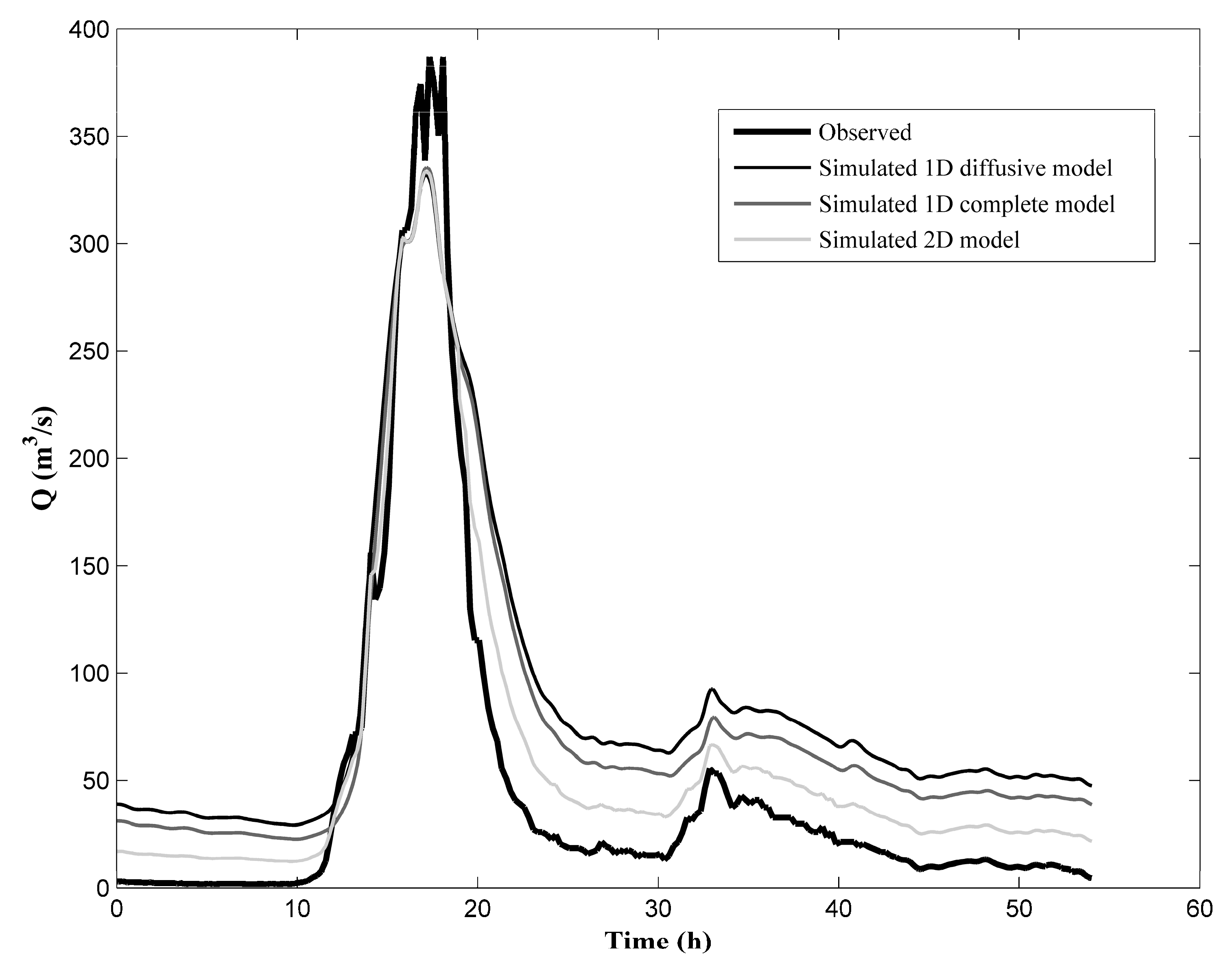
In the paper, we make a distinction between ‘hard’ and ‘soft’ data [8,9]. By ‘hard’ we mean data that are a direct measure of a physical variable, in our case only the water stage measured in the two gauged sections during the event; by ‘soft’ we mean data that are inferred from measures of different variables and are affected by a large uncertainty, in our case discharge hydrographs at the same gauged sections obtained from existing rating curves. The validation of the methodology is based on (1) comparison between the results of three different hydraulic models and the ‘hard’ measured water level data, (2) comparison of the model results with the remaining ‘soft’ data. Because reliable ‘hard’ rating curves are not available, the validation of the methodology is based on (1) ‘soft’ data coming from hydrological rainfall–runoff models or the available rating curves; (2) comparison between the results computed using three different hydraulic models and the ‘hard’ measured water level data.

2. The Reverse Flow Routing Problem

In the methodology proposed by [7], the discharge hydrographs are computed as solution of a flow routing problem, solved along a domain of some kilometers, where the upstream boundary condition is given by the stage hydrograph measured in the reach upstream section. The zero diffusion downstream boundary condition is set in a river section located some hundred meters downstream of the second gauged section, far enough to avoid any significant inference with the stages here computed. A numerical hydraulic model provides the relationship between the measured upstream stage hydrograph and both the stage and discharge hydrographs in all the sections. Initial conditions are almost irrelevant if measures are available shortly before the sought-after investigation time.

If one or more tributaries flow into the investigated reach between the two gauged sections, the corresponding discharge $Q_j^T$ is estimated as:

$$Q_j^T=K_j^T(H_j)C_j,$$

(1)

where j is the tributary index, $K_j^T(H_j)$ is the conveyance—that is the discharge per unit energy slope and per unit roughness coefficient—H_j is the water stage in the inlet section of the main reach and C_j can be considered as a calibration parameter accounting for both the energy slope, S_j, and the bed roughness along the tributary. If linearity occurs between the inverse of the average Manning coefficient and the specific discharge, parameter C_j will be equal to:

$$C_j=\frac{\sqrt{S_j}}{n^T}.$$

(2)

Model parameters are the Manning coefficient n and the tributary parameters C_j. They are calibrated by searching the best match between the computed stage hydrograph in the second gauged section and the measured one.

3. Hydraulic Models

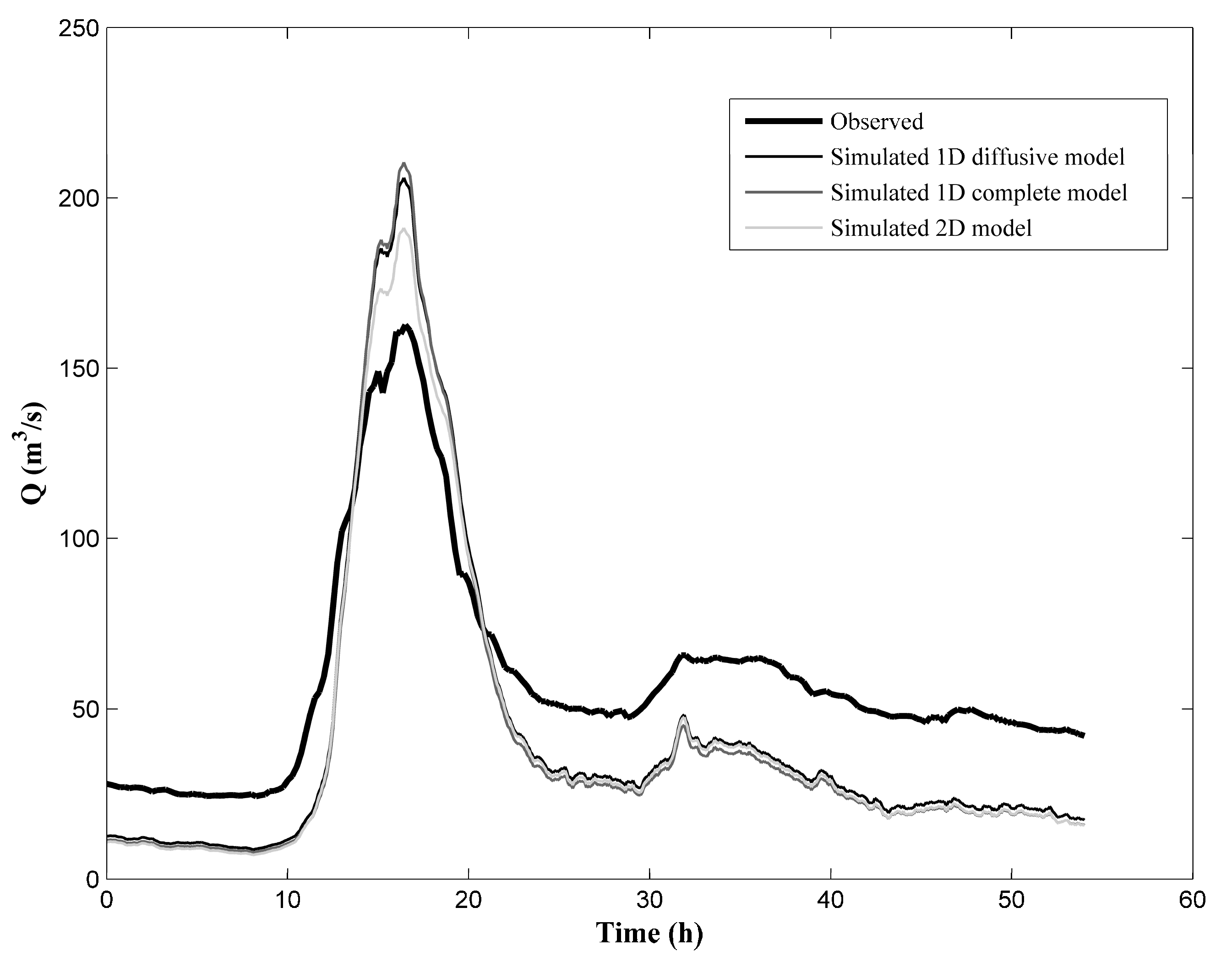
The link between the input stage hydrograph in the upstream section and the computed one in the downstream measurement section is provided, for each trial parameter set, by the hydraulic model. In order to investigate about the robustness of the adopted model with respect to the sought after discharge estimation, three different options have been tested. Model 1: Complete 1D model; Model 2: Diffusive 1D model; Model 3: Diffusive 2D model.

All the models have been solved using the MAST numerical technique [10,11], assuming a piece-wise linear variation of water levels and discharges between sections in the 1D model and inside elements of an unstructured triangular mesh in the 2D model. Optimization of tributary parameters C_j has been carried out only with the 1D models and the tributary discharges computed with the 1D diffusive model have been assigned to the tributary inflow nodes of the 2D diffusive model.

3.1. Model 1: Complete 1D Model

Saint Venant governing equations of the 1D model are:

$$\frac{\partial A}{\partial t}+\frac{\partial Q}{\partial x}=p,$$

(3)

$$\frac{\partial Q}{\partial t}+\frac{\partial (Q^2/A)}{\partial x}+gA\frac{\partial h}{\partial x}+gA(S_f-S_0)=0,$$

(4)

where Q is the discharge in the main river, A is the cross-section area, h is the water depth, p is the lateral inflow per unit length (assumed normal to the flow direction), S₀ is the bottom bed slope and S_f is the friction slope. Friction slope is estimated according to the uniform flow formula, that is:

$$S_f=\frac{Q^2}{K^2},$$

(5)

where K is the conveyance—that is the river discharge according to uniform-flow condition and unit bottom slope—and g is set equal to 9.81 when the international unit system is adopted. Conveyance K is computed as function of the Manning coefficient n, the geometry of the river section and the water depth h, according to [6]. The investigated reach is discretized in N − 1 channels, linking N sections at the centre of N computational cells. The water depth in each section and the discharge in each channel are computed at each time level k + 1 starting from the known values at level k according to a prediction-correction approach, named MAST (MArching in Space and Time). In the prediction step the piezometric gradients of each computational element between two sections are kept constant in time, as computed at the end of the kth time step and governing equations are solved in the form of ordinary differential equations one computational cell after the other.

The correction step leads to the solution of a simple, very well conditioned diffusive problem of order N. Details of the mentioned procedure can be found in [8].

Some computational sections are located on weirs. Because in the prediction step a fully upwind scheme is used, the geometry of the section immediately downstream the weir is assigned to the ith element between sections i and i + 1, and the piezometric gradient in the upstream channel between sections i − 1 ad i during the prediction step is computed as:

$$\frac{\partial \left(z+h\right)}{\partial x}\approx \frac{\max \left(z_{w,i}+C{r}_i,z_i+h_i^k\right)-z_{i-1}-h_{i-1}^k}{L_{i,i-1}}.$$

(6)

where L_i,i−1 is the length of the element i − 1 between sections i − 1 and i, z_w,i is the minimum level of the weir sill, $h^k{}_{i-1}$ is the water depth computed at time level k and Cr_i is the minimum between the critical depth of the discharge in the upstream element i − 1 and its water depth, computed at time level k. If the first argument of the max function is the maximum one, free-fall conditions hold on the weir. In this case the water stage in section i is assumed to be the stage downstream of the weir, and in the next corrective step the diffusive flux entering in cell i from the upstream element is neglected. In the other case, continuity is assumed to hold in section i between the stages of the elements i − 1 and i.

3.2. Model 2: Diffusive 1D Model

According to several researchers [12,13,14], the inertial terms in the momentum Equation (4) can be neglected in the computation of the propagation of most of the natural events, as shown in [15] for the Tiber and the Arno River, leading to the so-called diffusive model. The use of the diffuse model instead of the complete one has several advantages. The first advantage is that water levels, or their spatial derivatives, are always suitable boundary conditions at the two ends of the model and the previously mentioned calibration procedure can always be carried out as explained in the introduction even if supercritical conditions hold in the upstream or in the downstream section; the second advantage is that the sensitivity of the computed water levels with respect to the topographic error is smaller for the diffusive model than for the complete one. This implies that the results of the diffusive model, unless very precise information on the river bed morphology are available, are likely to be more precise than the results of the complete model.

On the other hand, the input flux variability during the two mentioned test cases in Italy (Tiber and Arno basin flood events), as well as during most of the events in hydrological basins located in the central and northern part of Europe, is usually much lower than the input flux variability in small basins located in the southern part of Europe. This suggests the opportunity of checking out the difference between the results obtained using the two models for the analysis of the events in a case study characterized by torrential flow regime, the Crati River. Observe that the diffusive model can be derived from the complete one by increasing indefinitely the gravity acceleration g in Equation (4), which turns the same equation into:

$$\frac{\partial h}{\partial x}+S_f-S_0=0.$$

(7)

Use of the MAST technology also allows to differentiate the gravity acceleration term along the domain, from the minimum 9.81 value (in the IS unit system) to the infinite asymptotic value. In this last case, the critical water depth Cr_i in Equation (6), for sections in the weir location, becomes infinitesimal.

3.3. Model 3: Diffusive 2D Model

The previously mentioned 1D models rely on the assumption of neglecting the velocity components along the horizontal direction normal to the main stream direction, and also of approximating to 1.0 the average kinetic energy and momentum flux coefficients. Both hypotheses are questionable in the case of floods, when large flat areas can be inundated at the peak time. In order to compare the results obtained by the 2D model with the previous ones, the same MAST procedure has been applied [9] to find the solution of the diffusive approximation of the 2D Saint Venant equations, that are:

$$\frac{\partial hu}{\partial x}+\frac{\partial hv}{\partial x}-\frac{\partial h}{\partial t}=0,$$

(8a)

$$\frac{\partial hu}{\partial x}+\frac{\partial hv}{\partial x}-\frac{\partial h}{\partial t}=0,$$

(8b)

$$\frac{\partial h}{\partial y}+S_{f,y}-S_{0,y}=0,$$

(8c)

where u and v are the vertically averaged velocity components in the x and y direction, respectively; S_0,x and S_0,y are the ground slope in the x and y directions, respectively; and S_f,x , S_f,y are the bottom friction components in the x and y directions, computed as:

$$S_{f,x}=u\sqrt{u^2+v^2}\frac{n^2}{h^{4/3}},$$

(9a)

$$S_{f,x}=u\sqrt{u^2+v^2}\frac{n^2}{h^{4/3}},$$

(9b)

Equations (8) and (9) can be solved inside a 2D domain around the river bed axis including all the potentially inundated area. The domain is laterally bounded by an arbitrary line located in the always dry area, as well as by the trace of the upstream and downstream sections. A triangular unstructured mesh is used for the domain discretization. The water depth is given as boundary condition at all the nodes on the trace of the upstream section, and the diffusive fluxes leaving the boundary nodes on the trace of the downstream section are neglected. Impervious boundary conditions are assigned to the lateral, dry boundary. Zero water depth is assigned to all the nodes as initial condition.

In the proposed 1D models, tributary inlet discharges are computed as the product of a parameter times a known function of the main river water stage at the inlet section. For the sake of simplicity, in the 2D model the discharge hydrographs computed using the optimal diffusive 1D model have been distributed among the nodes of the boundary of the 2D model located along the trace of the inlet tributary sections.

4. Case Study

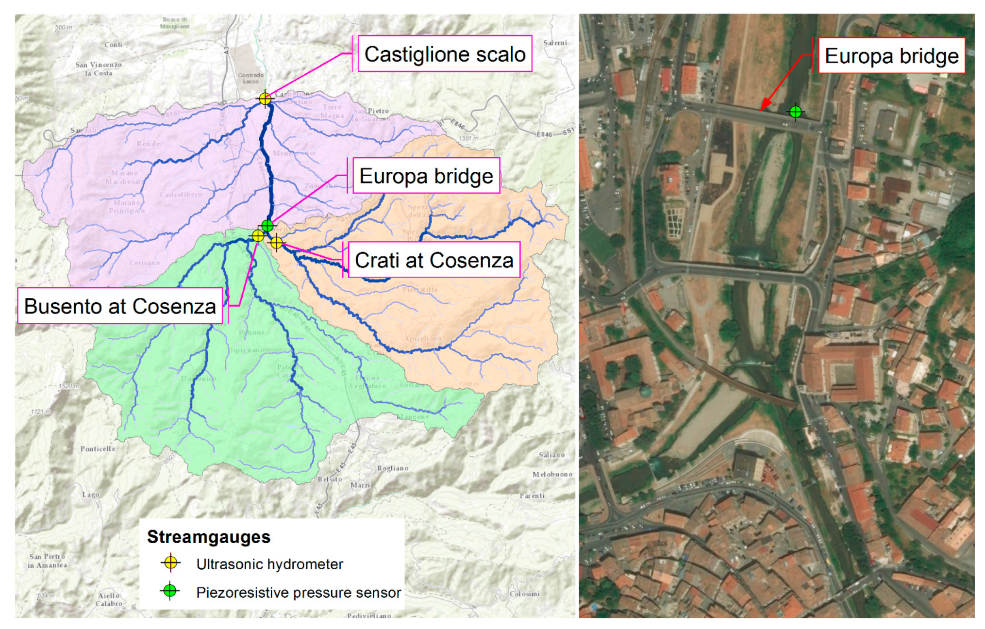
The upper Crati River basin, located in the Calabria region of southern Italy (Figure 1) is selected as the case study. The Crati River catchment represents the largest basin in the region; it originates from the western part of the Sila Mountains, at around 1700 m altitude, descends steeply northward, runs through the city of Cosenza, where the catchment area doubles in size thanks to the confluence on the left of the Busento River, and then flows into the Ionian Sea. The investigated reach is about 10 km long and is located in the urban area of the city of Cosenza starting from the section at the ‘Europa’ bridge, immediately after the confluence with the Busento River, with an initial catchment area of approximately 270 km². The selected reach is bounded downstream by the section of Crati at ‘Castiglione Scalo’, which drains a total area of about 400 km² and has been equipped since 1999 with an ultrasonic hydrometer managed by the public environmental protection authority.

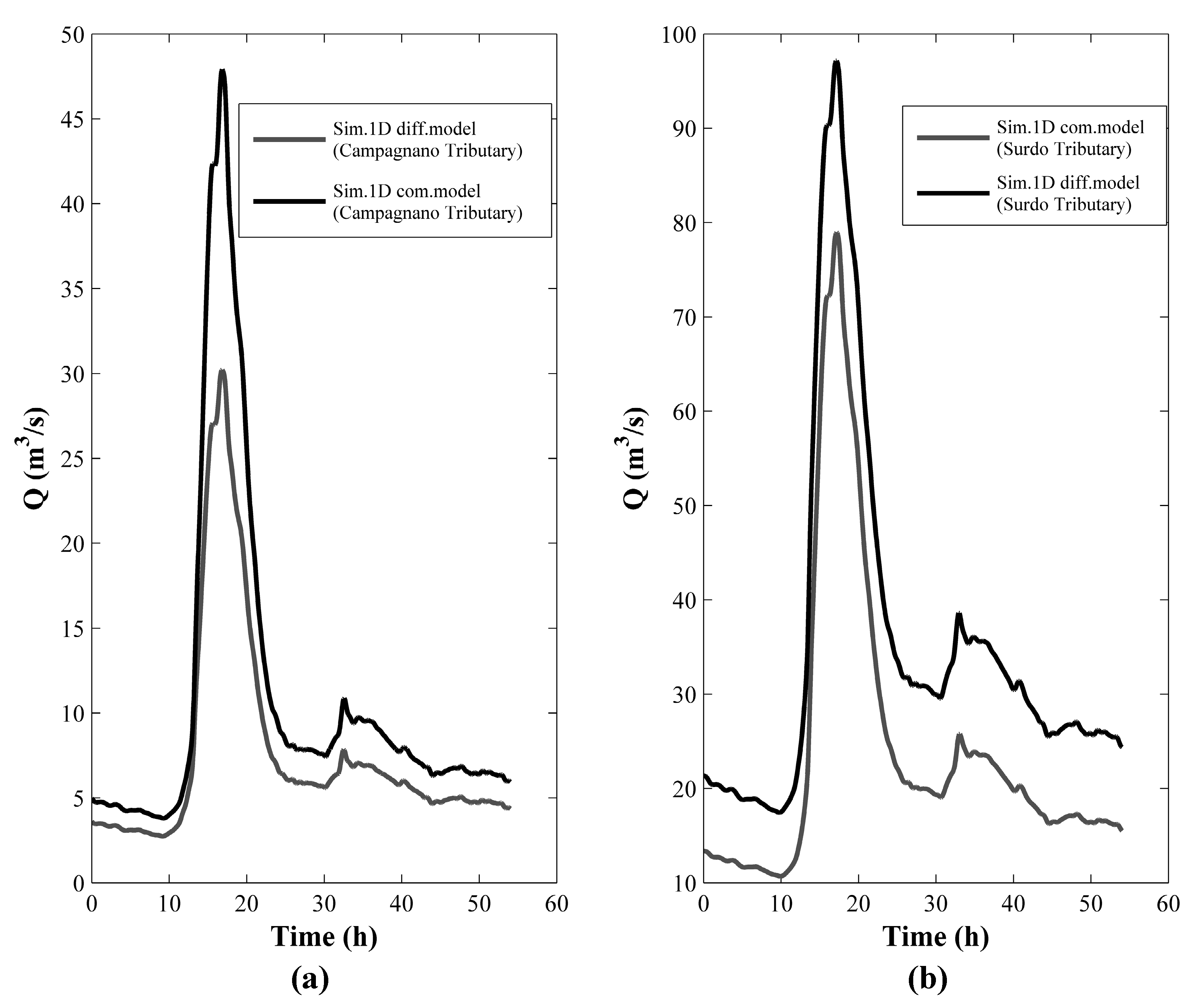
Along this reach we can find the confluence of several small tributaries. The two main ones are the Campagnano and the Surdo creeks (32 km² and 49 km² respectively), that join the Crati River at approximately the middle and the end of the reach. Many other ones, for a total catchment area of about 50 km², have small cross sections and are not accounted for in the present study.

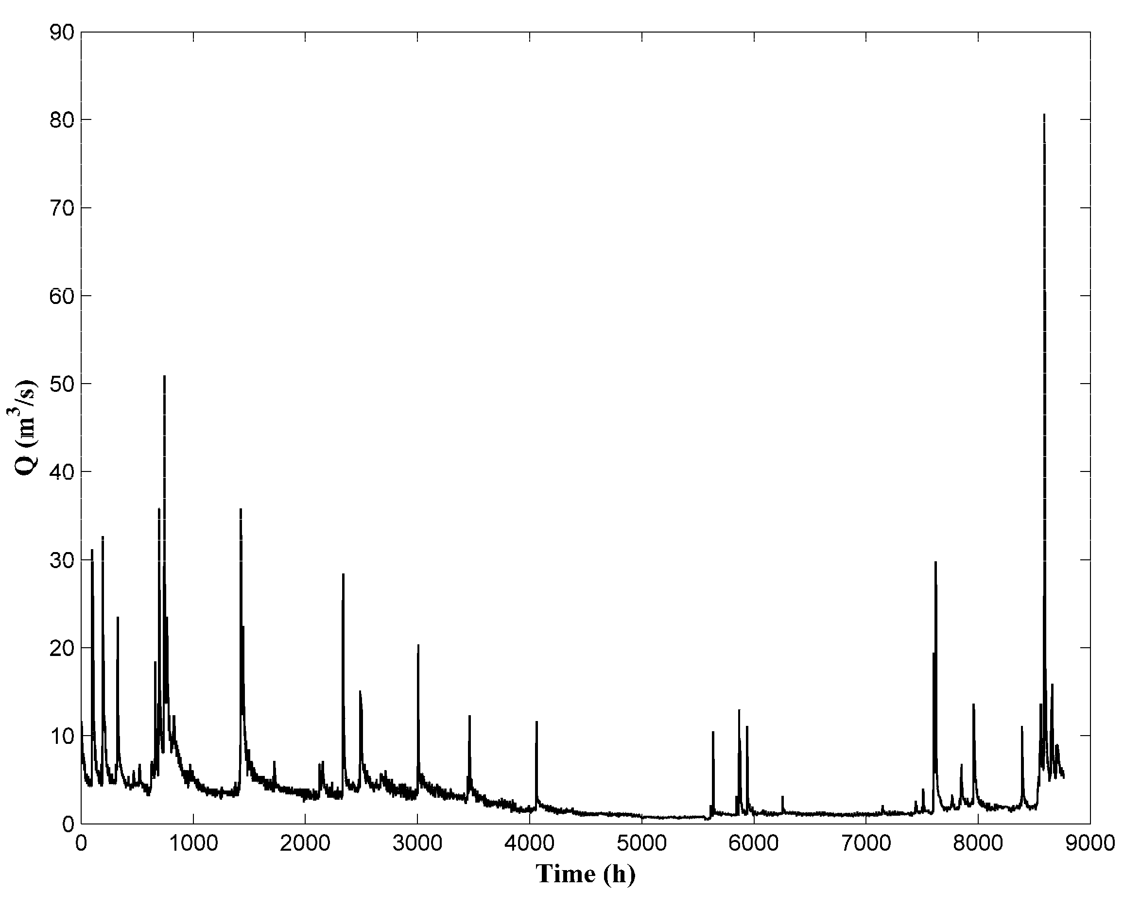
The river basin has a torrential regime, alternating long periods of low water levels during summer season to rapidly rising level closely related to flood events (e.g., 1951, 1953, 1959 and most recently in 2008). Historical discharge hydrographs are available at the ‘Castiglione Scalo’ hydrometric station, but original measured points are not available. For the reason explained in the introduction these data are likely to be affected by a large error and have to be considered as ‘soft’ data. The discharge hydrograph of year 2001 shown in Figure 2 confirms the hydrological behavior described above, with a maximum flow (80.7 m³/s) much higher than the average flow rate (3.2 m³/s) estimated for that year.

The upstream ‘Europa Bridge’ section was instrumented in 2010 with a piezoresistive pressure sensors Dipper-3 SEBA Hydrometrie, with an operating range of 10 m, an accuracy of ±0.05% and a resolution of 0.3 mm.

As shown in Figure 1, in addition to the downstream ‘Castiglione Scalo’ section, two other monitoring stations of the Calabria hydrological monitoring network are nearby the investigated reach, namely the ‘Busento River’ and the ‘Crati at Cosenza’ stations, located upstream the confluence of the two rivers.

A high resolution Digital Terrain Model (DTM) with cell size of one meter derived from Airborne LiDAR survey promoted by the Italian Ministry for Environment, Land and Sea (Ministero dell’Ambiente e della Tutela del Territorio e del Mare, MATTM) was used for the topographic description of the area. In 1D models the reach has been discretized with a total number of 69 cross sections (see Figure 3) extracted from the available DTM with a very small spacing using a semi-automatic tool available on GIS environment. Digital information has also been conveniently integrated with several in-situ surveys. The distance between two consecutive sections near bridges was adequately reduced to provide reliable reconstruction of the bed profile and weirs have been modelled according to the description given in Section 3.1. The 1D and 2D model domains have been extended about 500 m after the gauged ‘Castiglione Scalo’ section in order to minimize the effect of the approximation used in the applied downstream boundary condition.

The study case is a flood that occurred during winter 2016, between 12 February and 14 February. The main characteristics of the selected event are summarized in

Table 1. Main characteristics of the 2016 event in the Crati River at Europa Bridge and Castiglione Scalo.

Event	ΔT (h)	Europa Bridge		Castiglione Scalo
		Qp (m3·s−1)	tp (h)	Qp (m3·s−1)	hp (m)	tp (h)
February 2016	54	162.72	16.50	386.7	1.78	17.16

, where Q_p is the peak discharge, h_p is the peak stage, t_p is the peak time, and ΔT is the flood duration event (‘soft’ data).

The cumulated mean areal precipitation over the basin at Castiglione Scalo was equal to approximately 90 mm and triggered a river flood with inundations in some areas downstream of the gauged reach.

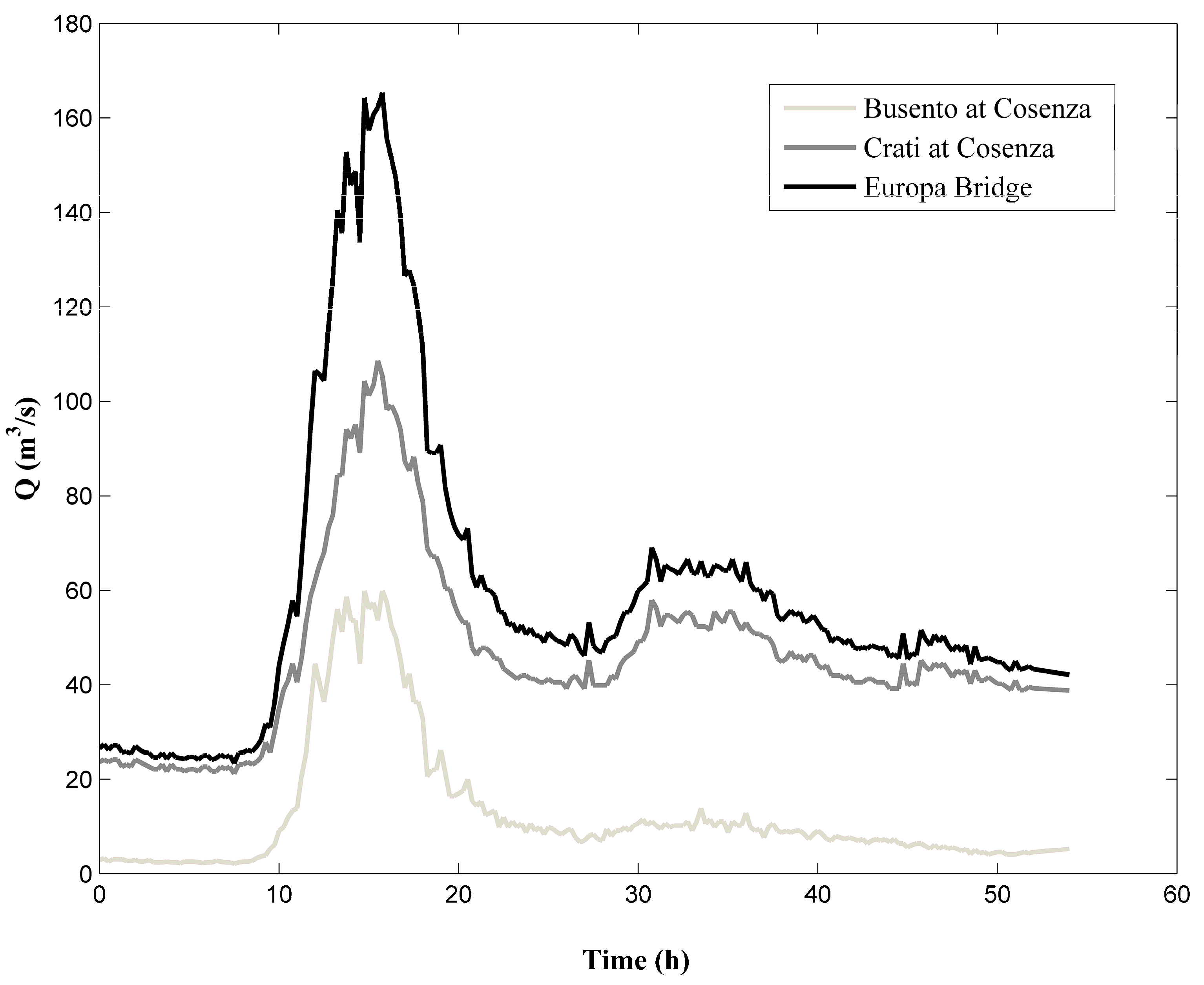
Figure 4 shows the estimated ‘soft’ discharge hydrographs used for validation, collected with 15-min intervals at the monitoring sites of Busento River station and Crati at Cosenza station. The discharge hydrograph at Europa Bridge, i.e., at the beginning of the investigated stretch, was estimated from this information as the sum of the two hydrographs and used in the following investigations (Figure 4, black line).

No information is available about the historical discharge flowing into the Crati from the Campagnano and Surdo creecks.

5. Results and Discussion

5.1. Parameter Calibration

In this paper, the Nash Sutcliffe efficiency coefficient [16] has been used for calibration, expressed by:

$$N{S}_h=\left[1-\frac{{\displaystyle {\sum }_{i=1,N}{(h_{i\_obs}-h_{i\_sim})}^2}}{{\displaystyle {\sum }_{i=1,N}{(h_{i\_obs}-{\overline{h}}_{obs})}^2}}\right].$$

(10)

where $h_{i\_obs}$ is the ith element of the observed stage hydrograph, $h_{i\_sim}$ is the ith element of the simulated stage hydrograph, ${\overline{h}}_{obs}$ is the mean observed stage and N is the total number of hydrograph time ordinates. NS_h can range from −∞ to 1, with a perfect fit obtained for NS_h = 1. The advantage of using the NS_h measure instead of the root mean square error (RMSE) is that it is dimensionless and its optimum value carries useful information about the relative estimation error associated to the optimal solution.

The time interval of the hydrograph used for calibration starts at the beginning of the rising limb and ends at the peak time, where the maximum time gradient occurs. This allows a larger sensitivity of the difference between the measured and the observed data with respect to the unknown wave time shift. Almost all the ‘goodness of fit’ indices available in literature measure the match between the computed and the measured hydrographs as a linear function of the quadratic errors. This leads to the conclusion that, generally, calibration provides a better fitness during the peak region of the stage hydrograph [17], which is a desirable property for the specific problem.

The case study selected in the Crati River basin has been modeled assuming a single roughness parameter, n, and two tributary constant C₁ and C₂ relative to the Campagnano and Surdo creeks in the 1D models. The roughness n is the only parameter in the 2D model. The motivation of this choice is that relationship given by Equation (1) assumes a single piezometric level in all the sections (which is of course not the case in the 2D model) and its extension to the 2D model would have required a much larger number of parameters. The simplified approach outlined in Section 3 is also based on the similarity between the results of the 1D and the 2D diffusive models discussed in the next section.

The NS_h optimal values are 0.878 and 0.709 for respectively the 1D diffusive and the 1D complete model (

Table 2. NS_h for optimized and perturbed parameters (±5%) in the 2016 event.

Model	Event	NSh	NSh (+5%)	NSh (−5%)	Tcal (h)
1D Diffusive	February 2016	0.878	0.868	0.861	8-18
1D Complete	February 2016	0.709	0.701	0.703	8-18
2D model	February 2016	0.854	-	-	8-18

), and 0.854 for the 2D diffusive model. The computed and the measured stage hydrographs are compared in Figure 5. The water stage of the downstream gauged section is assumed in the 2D model to be equal to the water stage computed at the node on the trace of the same section with the lowest topographic elevation.

5.2. Comparison of the Three Model Results

We observe first that the best fit is obtained with the 1D and 2D diffusive models, as already observed in previous studies. Both complete and diffusive models provide higher slopes of the stage hydrograph with respect to the measured one, and this is likely due to the existence of a lateral distributed inlet flow, not accounted for in the adopted conceptual model. We also observe that the results of the 2D model, obtained using the same Manning coefficient of the 1D diffusive model are very similar to the previous ones along the rising limb and the shift from 1D to 2D modeling, which is computationally very expensive, does not provide a significant improvement. The difference between the water stages in the 1D and the 2D models before and after the rising limb can be explained with the effect of the different spatial discretization of the river bed topography, which is more effective in the case of low water depths.

The optimal values of the three parameters n, C₁ and C₂, able to closely reproduce the stage hydrograph observed at Castiglione Scalo section, are summarized in

Table 3. Calibration parameter values for the 2016 event.

Model	Event	n (s·m−1/3)	n+5% (s·m−1/3)	n−5% (s·m−1/3)	C1 (-)	C1+5% (-)	C1−5% (-)	C2 (-)	C2+5% (-)	C2−5% (-)
1D Diffusive	February 2016	0.0500	0.0525	0.0475	0.900	0.945	0.855	1.900	1.995	1.805
1D Complete	February 2016	0.0560	0.0588	0.0532	1.100	1.155	1.045	1.200	1.260	1.140

for the investigated event. The optimal n parameter in the 2D model is equal to 0.065. The effects of small perturbations of these parameters, for both 1D diffusive and 1D complete models, have been also assessed in terms of variations of the NS_h measure computed at Castiglione Scalo, by increasing or lowering all the model parameters by five percent. See perturbed parameters in Table 3 and resulting NS_h values in Table 2.

Figure 6a–c, for the 1D diffusive model, plot the Nash and Sutcliffe efficiency as function of the n, C₁ and C₂ parameters around their optimal values.

Observe that the change of the three parameters affects differently the computed stage hydrographs. Specifically, the increment of the Manning coefficient, n, leads to a reduction of both the peak time and the stage hydrograph volume; on the opposite, the value of the tributary constants C₁ and C₂ mainly affects the volume of the computed hydrographs. In spite of this, equifinality of the parameters with respect to the sought after measure clearly plagues the problem [7]. See in Table 2 that similar values of the sought after NS_h measure are obtained with a five percent variation of all the parameters.

Due to the uncertainty in the available discharge data, the most significant measure of the capability of each single model in reproducing the relationship between the upstream stage and discharge hydrographs is given by the NS_h measure, obtained using ‘hard’ water level data in the downstream section. We observe first that Model 2 (Diffusive, 1D) and Model 3 (Diffusive, 2D) provide the best NS_h value, almost equal to 0.88 and 0.85, which is much better than the value 0.71 obtained using Model 1 (Complete, 1D). This is consistent with previous results documented, for example in [7], and can be explained with the motivation given in Section 3.2. A sensitivity analysis is also carried out to test the robustness of the NS_h measure with respect to small (five percent) parameter changes. We can see in Table 2 and Table 3 that the relative change of the NS_h measure is much smaller than the relative change of the input parameters. On the other hand, any improvement is missing in the application of the 2D model, against a significant increment of the computational cost. This can be explained by the topography of the river bed and by the resulting small extension of the flooded areas. See the inundated area around the two gauged sections, computed by the 2D model, in Figure 7a,b.

Finally, observe that the optimal n parameter in the 2D model (0.065) is higher than in the 1D model (0.055). The explanation is that the global resistance computed in each river section by the 2D model is equivalent to the resistance computed by a 1D model using the Divided Channel Method and this method is well-known to underestimate, for a given n, the total resistance [6].

5.3. Model Validation with Respect to the ‘Soft’ Historical Data

Two performance criteria have been used for the estimated upstream and downstream discharge hydrographs. The considered performance metrics are the relative magnitude peak error and the Nash Sutcliffe efficiency coefficient. When applied to the discharge hydrograph they are calculated as follows:

$$\mathrm{Relative\; magnitude\; peak\; error}:\Delta Q_p=\left[\frac{{Q_p|}_{sim}}{{Q_p|}_{obs}}-1\right]\times 100$$

(11)

$$\mathrm{Nash\; Sutcliffe\; efficiency\; coefficient}:N{S}_q=\left[1-\frac{{\displaystyle {\sum }_{i=1,N_e}{(Q_{i\_obs}-Q_{i\_sim})}^2}}{{\displaystyle {\sum }_{i=1,N_e}{(Q_{i\_obs}-{\overline{Q}}_{obs})}^2}}\right]$$

(12)

where Q_p and Q_i are the peak discharge value and the ith element of the discharge hydrograph, respectively, N_e is the number of data in all the hydrograph and $\overline{Q}$ is the mean discharge value. Subscript _sim and _obs refer to estimated and observed data, respectively.

Figure 8 shows, for the investigated event, the comparison between the discharge hydrographs computed using the optimal n and C parameter values (obtained for the 1D models and 2D model) and the observed ones at the ‘Europa Bridge’ section, while Figure 9 shows the comparison between discharge hydrographs computed and estimated at Castiglione Scalo and Figure 10 shows the tributaries’ hydrographs computed with the diffusive and the complete 1D models. Observe that results of the two 1D models for each of the two tributaries are quite different, specially for the Campagnano creek. This is likely due to the different optimal values obtained for the corresponding C parameter, as reported in Table 3.

It is very important to point out that, in spite of the equifinality of the model parameters with respect to the NS measure, the corresponding estimated discharge hydrograph in the upstream and downstream sections are very stable around the calibrated set of parameters. See in

Table 4. Crati River, performances in terms of Nash Sutcliffe index NSQ, RMSE and relative magnitude peak error, ΔQp.

Models	Europa Bridge, Discharge					Castiglione Scalo, Discharge
	NSQ	NSQ+5%	NSQ−5%	RMSE (m3·s−1)	ΔQp (%)	NSQ	NSQ+5%	NSQ−5%	RMSE (m3·s−1)	ΔQp (%)
1D diffusive	0.50	0.512	0.497	22.87	20.97	0.68	0.665	0.676	47.11	13.76
1D complete	0.41	0.397	0.377	24.74	22.33	0.78	0.756	0.774	38.65	13.28
2D	0.65	-	-	20.19	14.42	0.723	-	-	24.22	14.24

the NS_q indices computed by means of a five percent increment or reduction of all the parameters of each 1D model. Even if ‘soft’ data are a poor data source for validation, perturbation analysis has shown the robustness of the estimated discharges with respect to the optimal parameter uncertainty.

The performances of the computed hydrographs are reported in Table 4.

6. Conclusions

The unsteady state water level data analysis for the estimation of the discharge hydrograph in a selected reach of the Crati River, where ‘hard’ discharge measurements are missing, has given the opportunity to compare the results provided by three different hydraulic models and to get the following indications, consistent with other previous analysis:

• The diffusive 1D model has shown a good performance in estimating the downstream stage hydrograph, even if a clear effect of a distributed lateral flow, not accounted for in all the hydraulic models, is present;
• The performance of the 1D diffusive model is much better than the performance of the complete one, according to the Nash-Sutcliffe measure of the downstream ‘hard’ water level data;
• The diffusive 2D model does not provide any improvement of the water level computed in the downstream section; this could be due, in this specific case, to the small extension of the flooded area.
• Even if parameter models are plagued by equifinality with respect to the Nash-Sutcliffe measure, the discharge hydrograph estimation is very robust around the optimal parameter set.

References

1. Cunge, J.A.; Holly, F.M.; Verwey, A. Practical Aspects of Computational River Hydraulics; Pitman Advanced Publishing Program: London, UK, 1980. [Google Scholar]
2. Bonacci, O. Several methods for discharge measurements of floods/Plusieures méthodes de mesure du débit des crues. Hydrol. Sci. J. 1983, 28. [Google Scholar] [CrossRef]
3. Polemio, M.; Petrucci, O. The occurrence of floods and the role of climate variations from 1880 in Calabria (Southern Italy). Nat. Hazards Earth Syst. Sci. 2012, 12, 129–142. [Google Scholar] [CrossRef]
4. Nasello, C.; Tucciarelli, T. Dual multilevel urban drainage model. J. Hydraul. Eng. ASCE 2005, 131, 748–755. [Google Scholar] [CrossRef]
5. Aricò, C.; Sinagra, M.; Begnudelly, L.; Tucciarelli, T. MAST 2D diffusive model for flood prediction on domains with triangular Delaunay unstructured meshes. Adv. Water Resour. 2011, 34, 1427–1449. [Google Scholar] [CrossRef]
6. Spada, E.; Sinagra, M.; Tucciarelli, T.; Sammartano, V.; Corato, G. Computation of vertically averaged velocities in irregular sections of straight channels. Hydrol. Earth Syst. Sci. 2015, 19, 3857–3873. [Google Scholar] [CrossRef]
7. Spada, E.; Sinagra, M.; Tucciarelli, T.; Barbetta, S.; Moramarco, T.; Corato, G. Assessment of river flow with significant lateral inflow through reverse routing modeling. Hydrol. Process. 2017, 31, 1539–1557. [Google Scholar] [CrossRef]
8. Seibert, J.; McDonnell, J.J. On the dialog between experimentalist and modeller in catchment hydrology: Use of soft data for multicriteria model calibration. Water Resour. Res. 2002, 38, 1241. [Google Scholar] [CrossRef]
9. Winsemius, H.C.; Schaefli, B.; Montanari, A.; Savenije, H.H.G. On the calibration of hydrological models in ungauged basins: A framework for integrating hard and soft hydrological information. Water Resour. Res. 2009, 45, W12422. [Google Scholar] [CrossRef]
10. Aricò, C.; Tucciarelli, T. A Marching in Space and Time (MAST) solver of the shallow water equations. Part I: The 1D model. Adv. Water Resour. 2007, 30, 1236–1252. [Google Scholar] [CrossRef]
11. Aricò, C.; Nasello, C.; Tucciarelli, T. A Marching in Space and Time (MAST) solver of the shallow water equations. Part II: The 2D model. Adv. Water Resour. 2007, 30, 1253–1271. [Google Scholar] [CrossRef]
12. Perumal, M.; Moramarco, T.; Shaboo, B.; Barbetta, S. A methodology for discharge estimation and rating curve development at ungauged sites. Water Resour. Res. 2007, 43, W02412. [Google Scholar] [CrossRef]
13. Perumal, M.; Ranga Raju, K.G. Variable-parameter stagehydrograph routing method. I: Theory. J. Hydrol. Eng. 1998, 3, 109–114. [Google Scholar] [CrossRef]
14. Perumal, M.; Ranga Raju, K.G. Variable-parameter stagehydrograph routing method. II: Evaluation. J. Hydrol. Eng. 1998, 3, 115–121. [Google Scholar] [CrossRef]
15. Aricò, C.; Nasello, C.; Tucciarelli, T. Using unsteady water level data to estimate channel roughness and discharge hydrograph. Adv. Water Resour. 2009, 32, 1223–1240. [Google Scholar] [CrossRef]
16. Nash, J.E.; Sutcliffe, J.V. River flow forecasting through conceptual models, part 1: A discussion of principles. J. Hydrol. 1970, 10, 282–290. [Google Scholar] [CrossRef]
17. Legates, D.R.; McCabe, G.J. Evaluating the use of goodness-of-fit measures in hydrologic and hydroclimatic model validation. Water Resour. Res. 1999, 35, 233–241. [Google Scholar] [CrossRef]
Figure 1. Location of the investigated reach of the Crati River (Europa bridge–Castiglione Scalo) and of the river gauging stations.
Water 09 00288 g001
Figure 2. Streamflow time series for a typical year (2001) at Castiglione Scalo.
Water 09 00288 g002
Figure 3. Morphology of the Crati River basin with the location of the hydrometric gauged sections.
Water 09 00288 g003
Figure 4. Estimated discharge hydrographs at the monitoring sites of Busento and Crati river gauged sections and at Europa Bridge.
Water 09 00288 g004
Figure 5. Crati River, February 2016 flood: comparison between observed and computed stage hydrographs at Castiglione Scalo site (‘hard’ data).
Water 09 00288 g005
Figure 6. Castiglione Scalo section, 1D diffusive model: Nash Sutcliffe, NSh, versus: (a) C1 and n parameters for fixed optimum C2 parameter; (b) C2 and n parameters for fixed optimum C1 parameter; (c) C1 and C2 parameters for fixed optimum n parameter.
Water 09 00288 g006
Figure 7. Inundated area computed by the 2D model (a) at Europa bridge site and (b) at Castiglione Cosentino site.
Water 09 00288 g007
Figure 8. Comparison between observed and computed discharge hydrographs at Europa Bridge site for the 1D models and the 2D model (‘soft’ data).
Water 09 00288 g008
Figure 9. Comparison between observed and computed discharge hydrographs at Castiglione Scalo site for the 1D models and the 2D model (‘soft’ data).
Water 09 00288 g009
Figure 10. Comparison between the computed tributaries discharge hydrographs (Campagnano and Surdo) for the 1D models: (a) Campagnano; (b) Surdo.
Water 09 00288 g010