Stability Control for Electric Vehicles with Four In-Wheel-Motors Based on Sideslip Angle

Abstract

Tire longitudinal forces of electrics vehicle with four in-wheel-motors can be adjusted independently. This provides advantages for its stability control. In this paper, an electric vehicle with four in-wheel-motors is taken as the research object. Considering key factors such as vehicle velocity and road adhesion coefficient, the criterion of vehicle stability is studied, based on phase plane of sideslip angle and sideslip-angle rate. To solve the problem that the sideslip angle of vehicles is difficult to measure, an algorithm for estimating the sideslip angle based on extended Kalman filter is designed. The control method for vehicle yaw moment based on sliding-mode control and the distribution method for wheel driving/braking torque are proposed. The distribution method takes the minimum sum of the square for wheel load rate as the optimization objective. Based on Matlab/Simulink and Carsim, a cosimulation model for the stability control of electric vehicles with four in-wheel-motors is built. The accuracy of the proposed stability criterion, the algorithm for estimating the sideslip angle and the wheel torque control method are verified. The relevant research can provide some reference for the development of the stability control for electric vehicles with four in-wheel-motors.

1. Introduction

Unlike traditional vehicles and centralized-driving electric vehicles, electric vehicles with in-wheel-motors (IWMs) can save the chassis space and reduce the weight of vehicle effectively by integrating drive motors into wheel hubs and eliminating the drive shaft and other transmission parts. This makes it possible to equip a larger energy storage system and improve the ride comfort [1,2,3,4]. However, the use of IWMs results in a substantial increase in the unsprung mass of the vehicle and the moment of inertia for the driving wheels, which affects the handling and stability characteristics of the vehicle seriously. The vehicle stability control can solve the above problems and it plays an important role in vehicle active safety [5,6,7]. It is the basis for giving full play to the high performance of electric vehicles with IWMs [8]. At the same time, in terms of vehicle stability control, electric vehicles with four IWMs also have the following advantages: First, the driving torque and braking torque of each IWM can be adjusted independently [9,10]. The stability control can be achieved based on wheel torque vectoring control to improve the driving stability and maneuverability of electric vehicles with IWMs, but traditional vehicles and centralized-driving electric vehicles achieve the vehicle stability control mainly by controlling the driving forces of drive unit and differential braking forces [11,12]. Second, the adjusting speed and precision for IWM torque is better. The response delay for the motor torque control is among 20 to 30 ms, while the response delay for the electronic hydraulic brake system is among 50 to 60 ms [13]. Third, the motor torque can be calculated accurately [14,15], but the engine torque and hydraulic braking force mainly depend on the estimation. Therefore, the electric vehicle with four IWMs has great potential in improving the performance of vehicle stability control, such as control speed and control accuracy.

In recent years, with gradual maturity of the technology for centralized-driving electric vehicles, stability control for electric vehicles with IWMs has attracted the attention of scholars. The related research mainly focuses on two aspects: One is how to judge whether a vehicle is unstable or not. This is also one of the key problems for the stability control of centralized-driving vehicles. The other is how to use different control algorithms and strategies to give full play to the advantages of independent adjustable torque of the electric vehicles with IWMs. In judging whether a vehicle is unstable or not, the method of threshold values and the method of phase plane are commonly used. The method of threshold values uses the linear vehicle model with two degrees of freedom (2-DOF) to obtain the reference value of the yaw rate or the sideslip angle of vehicle. When the actual value of the yaw rate or sideslip angle exceeds its threshold value, the stability control system will work. However, compared with the actual state of the vehicle, the 2-DOF linear model makes a lot of simplification. Therefore, in a practical application, in order to ensure the effectiveness of the stability control, we often use a smaller threshold value for reliability, so as to narrow the effective working range of the stability control system. Therefore, the method of threshold values may cause frequent start and stop of the stability control system. The method of phase plane draws a phase trajectory according to the stability states of vehicle and divides the stability states of vehicle according to the phase-plane theory. It can avoid frequent start and stop of the stability control system. The non-linear vehicle model with 2-DOF is often used to draw the phase plane, because it is simple and can express the stability of the vehicle to a certain extent [16,17,18]. However, the nonlinear vehicle model with 2-DOF ignores the wheel rotation and body movement, and this still leads to errors between the calculated value and the actual value. The errors may cause judgment errors under certain working conditions. In making full use of the advantages of electric vehicles with IWMs, one of the common methods is to control the motor torque through coordinated work of different control subsystems. In the literature [19], the appropriate four-wheel angle and required yaw moment is obtained through the integrated control strategy, so that the vehicle’s yaw rate and sideslip angle can track its reference value well. Resources [20,21] took four-wheel independent driving electric vehicles as the research object and proposed a distribution strategy for motor torque and braking torque, which can improve the driving stability of the vehicle and reduce the demand for motor torques. The second method commonly used is to optimize the control algorithm to improve the accuracy and fault tolerance of the motor torque vectoring [15,22]. However, there is no consistent conclusion on how to make full use of the torque of each wheel [23], and how to make full use of the torque of each wheel is still the research focus of electric vehicles with IWMs.

In view of the above problems, this paper takes an electric vehicle with four IWMs as the research object. Firstly, the key problem in the vehicle stability control, that is, how to determine the vehicle is stable or not, is studied in depth. Sideslip angle ($\beta -\dot{\beta }$) phase planes are constructed by building a 7-DOF vehicle model, and this can improve the accuracy of the stability judgment basis. On the premise of considering key factors such as vehicle velocity and road adhesion coefficient, stability boundaries in phase planes are studied in depth, and a criterion for vehicle stability based on phase planes is established. Secondly, considering the problem that the sideslip angle is difficult to measure, the extended Kalman filter algorithm is selected to estimate the sideslip angle. The control method for vehicle yaw moment based on sliding-mode control and the distribution method for wheel driving/braking torque are proposed. The distribution method takes the minimum sum of the square for wheel load rate as the optimization objective. Finally, a cosimulation platform for an electric vehicle with four IWMs based on Carsim and Matlab/Simulink is built. Carsim is a mature commercial software, and it contains vehicle models with high precision. However, the Carsim software lacks the model for electric vehicles with IWMs. Therefore, on the basis of Carsim’ centralized-driving vehicle model and the IWM model based on Matlab/Simulink, a cosimulation model based on MATLAB/Simulink and Carsim is built to verify the accuracy of the proposed stability criterion, the algorithm for estimating the sideslip angle, and the wheel torque control method.

2. Vehicle Model

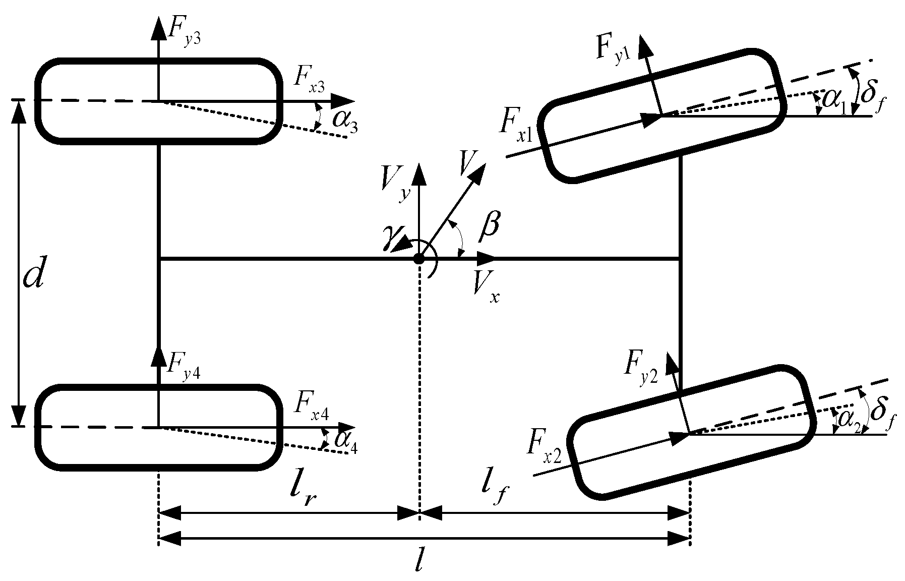
In this paper, a 7-DOF vehicle model is built, which includes longitudinal motion, lateral motion, yaw motion of vehicle body, and rotation of four wheels. The diagram of 7-DOF vehicle model is shown in Figure 1

When the front wheel angle is δ_f, longitudinal forces, lateral forces, and the yaw moment at the vehicle center of mass are as follows.

$${\displaystyle \sum F_{\mathrm{x}}=m({\dot{V}}_{\mathrm{x}}-V_{\mathrm{y}}\gamma )}=(F_{\mathrm{x}1}+F_{\mathrm{x}2})\cos {\delta }_{\mathrm{f}}-(F_{\mathrm{y}1}+F_{\mathrm{y}2})\sin {\delta }_{\mathrm{f}}+F_{\mathrm{x}3}+F_{x4}$$

(1)

$${\displaystyle \sum F_{\mathrm{y}}=m({\dot{V}}_{\mathrm{y}}-V_x\gamma )}=(F_{\mathrm{x}1}+F_{\mathrm{x}2})\cos {\delta }_{\mathrm{f}}+(F_{\mathrm{y}1}+F_{\mathrm{y}2})\sin {\delta }_{\mathrm{f}}+F_{\mathrm{y}3}+F_{\begin{array}{l}\mathrm{y}4\\ \end{array}}$$

(2)

$$\begin{array}{l}{\displaystyle \sum M_{\mathrm{x}}=I_{\mathrm{Z}}\dot{\gamma }=l_{\mathrm{f}}[(F_{\mathrm{y}1}+F_{y2})\cos {\delta }_{\mathrm{f}}-(F_{\mathrm{x}1}+F_{\mathrm{x}2})\cos {\delta }_{\mathrm{f}}]}\\ -l_r(F_{y3}+F_{y4})-\frac{d}{2}[(F_{y1}-F_{\mathrm{y}2}(\sin {\delta }_{\mathrm{f}}-(F_{\mathrm{x}1}-F_{\mathrm{x}2})\cos {\delta }_{\mathrm{f}}+F_{\mathrm{x}3}-F_{\mathrm{x}4}]\end{array}$$

(3)

Among them, F_xi and F_yi are calculated according to the magic formula tire model.

$$\{\begin{array}{l}{F}_{xi}({\lambda }_i)=x_{1\mathrm{x}}\sin \{x_{2\mathrm{x}}\arctan \left[x_{3\mathrm{x}}{\lambda }_i-x_{4\mathrm{x}}(x_{3\mathrm{x}}{\lambda }_i-\arctan (x_{3\mathrm{x}}{\lambda }_i))\right]\}\\ F_{yi}({\alpha }_i)=x_{1\mathrm{y}}\sin \{x_{2\mathrm{y}}\arctan \left[x_{3\mathrm{y}}{\alpha }_i-x_{4\mathrm{y}}(x_{3\mathrm{x}}{\alpha }_i-\arctan (x_{3\mathrm{y}}{\alpha }_i))\right]\}\end{array}$$

(4)

In Formulas (1)–(4), m is the mass of vehicle. I_z is the inertia moment of vehicle. V_x is the longitudinal velocity of vehicle. V_y is the lateral velocity of vehicle. γ is the yaw rate. δ_f is the front-wheel angle. l_f is the distance from the center of gravity to front axle. l_r is the distance from the center of gravity to rear axle. d is the wheelbase. F_xi is the longitudinal forces of each wheel and F_yi is the lateral forces of each wheel. Subscripts 1, 2, 3, and 4 indicate the left-front wheel, right-front wheel, left-rear wheel, and right-rear wheel respectively. λ_i is the tire slip rate. ${\alpha }_i$ is the sideslip angle of the tire. x_1x,x_2x,x_3x, and x_4x are the parameters determined by road conditions to get F_xi. x_1y,x_2y,x_3y, and x_4y are the parameters determined by road conditions to get F_yi.

The differential equation for the sideslip angle can be expressed as the following equation.

$$\dot{\beta }=\frac{{\displaystyle \sum F_y}}{m{V}_x}-{\displaystyle \mathrm{\int }\frac{{\displaystyle \sum M_z}}{I_z}}dt$$

(5)

where β is the sideslip angle and M_z is the yaw moment. The other letters are shown above.

3. Stability Criterion Based on $\beta -\dot{\beta }$ Phase Planes

Phase planes have been widely used to study the stability of nonlinear systems [24,25]. The vehicle is a typical nonlinear system, and the sideslip angle is the key parameter which can reflect its stability. The vehicle stability is greatly affected by factors such as vehicle velocities and road adhesion coefficients. Therefore, this paper analyzes the criterion of vehicle stability based on $\beta -\dot{\beta }$ phase planes under the premise of considering the key factors such as vehicle velocities and road adhesion coefficients.

3.1. Boundary Equation of $\beta -\dot{\beta }$ Phase Planes

According to the phase-plane theory, the $\beta -\dot{\beta }$ plane is divided into two parts: stable region and unstable region. In the stable region, any point on trajectories of vehicle motion state can quickly converge to the stable foci. That is to say, the vehicle can return to stable state by its own dynamic characteristics. In order to use $\beta -\dot{\beta }$ phase planes as the criterion of vehicle stability, we divide a phase plane into stable region and unstable region by using left and right boundary lines, the equation of boundary lines is:

$$\{\begin{array}{l}\dot{\beta }=-A\beta +B\\ \dot{\beta }=-A\beta -B\end{array}$$

(6)

Stable region of $\beta -\dot{\beta }$ phase planes can be expressed by the following formula:

$$\left|\dot{\beta }+A\beta \right|<B$$

(7)

In Formulas (6) and (7), A and B are coefficients related to structural parameters of a vehicle, driving states and road adhesion coefficients. Other letters are shown above. If Formula (7) is possible, the vehicle is running stably. Otherwise, it will lose its stability.

3.2. Influence of Driving Conditions on $\beta -\dot{\beta }$ Phase Planes

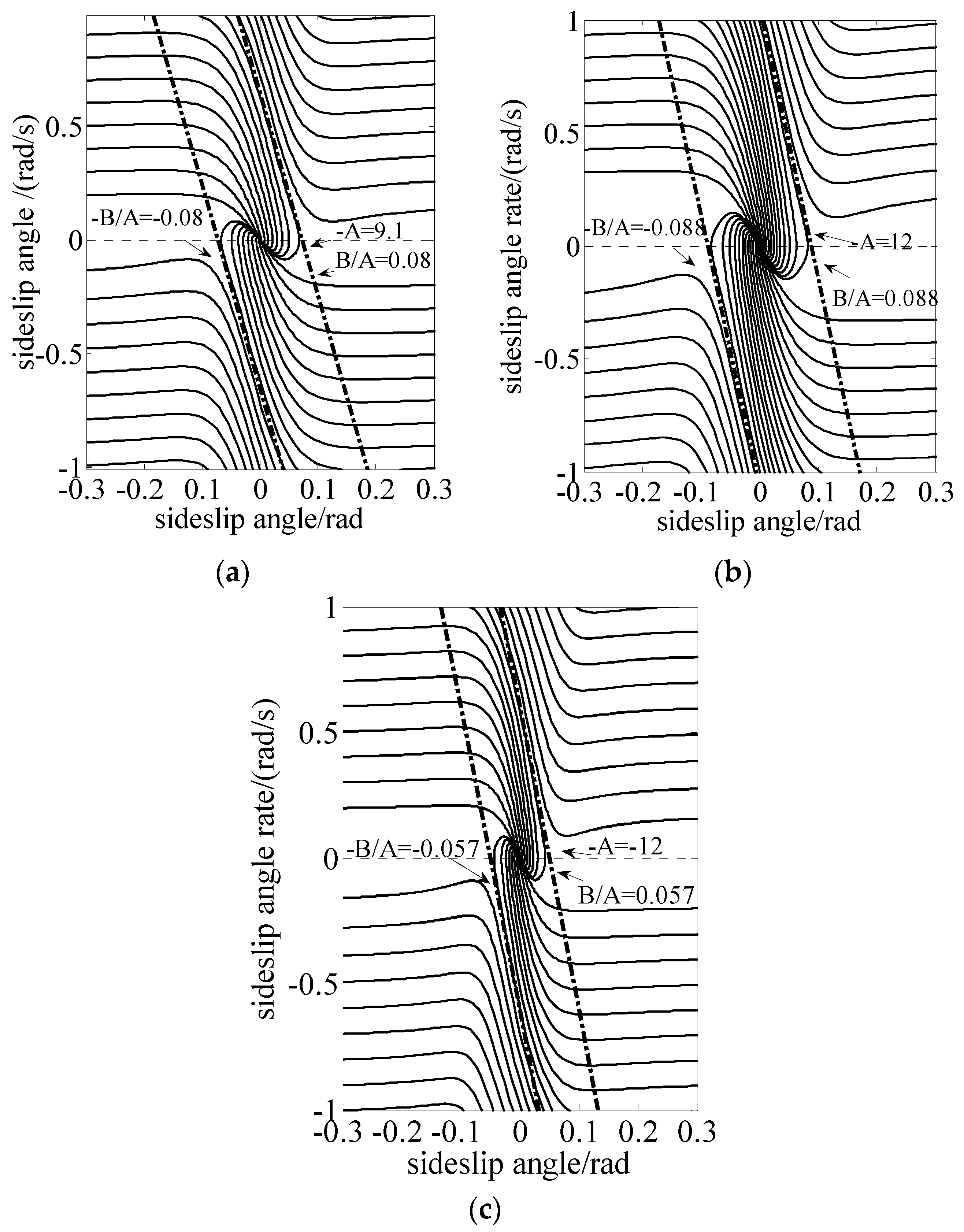
Phase trajectories in $\beta -\dot{\beta }$ phase planes change with vehicle driving states and road conditions, and the main influencing factors are road adhesion coefficients and vehicle velocities. Therefore, for comparative analysis 100 groups of phase portraits are drawn under different road adhesion coefficients from 0.1 to 1 and different vehicle velocities from 60 to 150 km/h. Taking $\beta -\dot{\beta }$ phase portraits of several typical driving conditions shown in Figure 2 as the example, the corresponding influencing factors are explained. In the figure, −A is the inclination of the boundary line, and −B/A and B/A are the intersection points of two boundary lines and the lateral axis, which are used to characterize the limit sideslip angle of the vehicle which $\dot{\beta }$ = 0. Compared with the Figure 2a–c, it can be seen that the absolute value of −B/A and B/A decreases with the increase of the vehicle velocity and the decrease of the road adhesion coefficient. The change of road adhesion coefficients has a greater influence on the size of stability region. When the absolute value of −B/A and B/A decrease, the stability region is reduced, and the vehicle is more likely to lose stability.

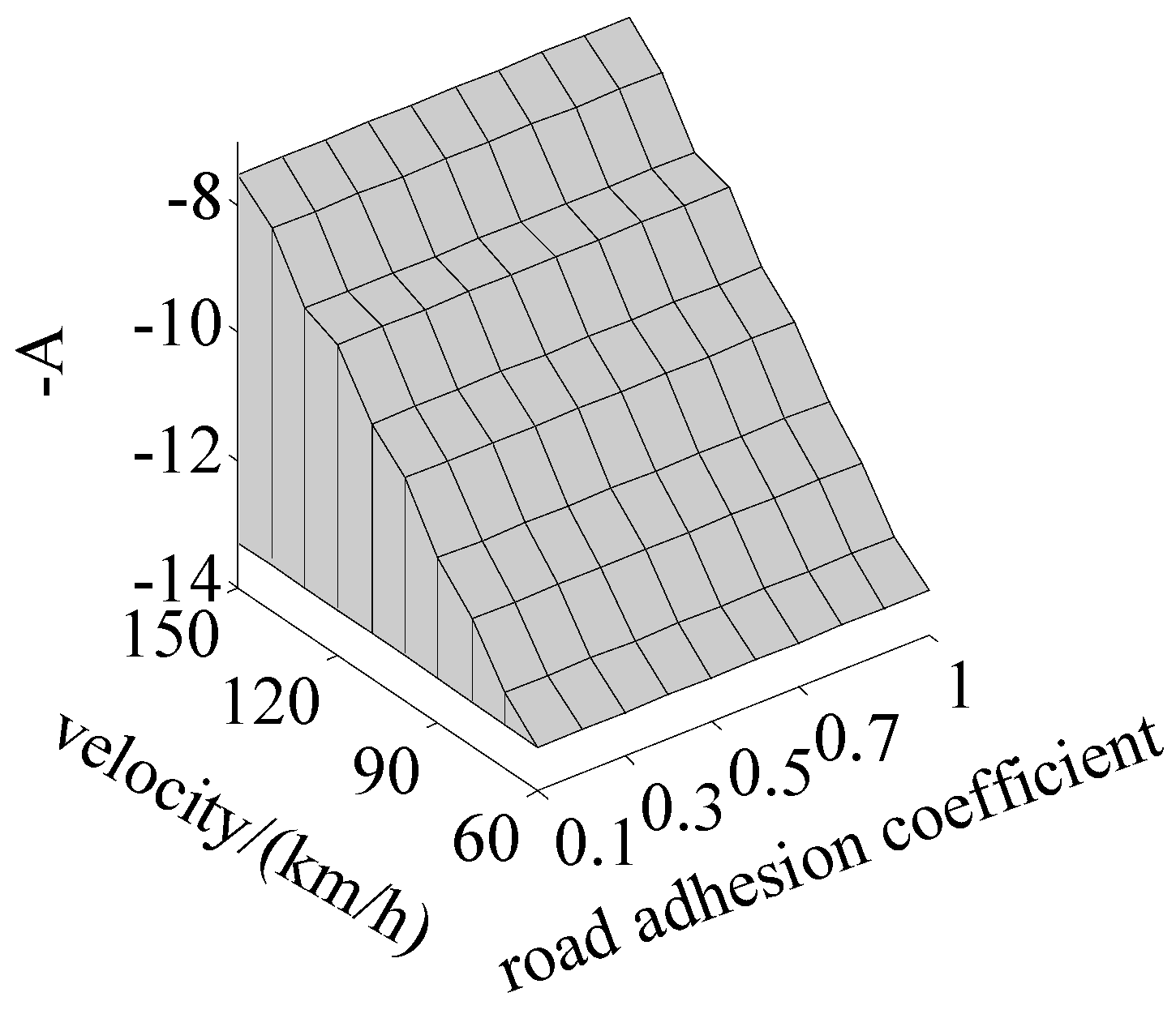
3.3. Parameters Determination for Boundary Lines of $\beta -\dot{\beta }$ Phase Planes

Based on the 100 groups of phase-plane diagrams drawn above, the intercepts and inclinations of 100 groups of boundary lines are obtained, and maps of the inclinations and intercepts are shown in Figure 3 and Figure 4. On the premise of considering the velocity and accuracy of simulation, the parameters of boundary lines can be determined by a two-dimensional look-up table according to the above maps and driving conditions, so as to reasonably judge the vehicle stability, based on $\beta -\dot{\beta }$ phase planes.

4. Estimation of Sideslip Angle

Although the vehicle stability can be judged by $\beta -\dot{\beta }$ phase plane effectively, the sideslip angle is difficult to be measured directly with cost-effective sensors [26]. Therefore, an algorithm is designed to estimate the sideslip angle based on extended Kalman filter. The corresponding extended Kalman filter consists of two processes: a prediction step and an update step. The prediction step is used to obtain the prediction state of the next time based on the current system state. The update step is used to obtain the optimal estimation of the system by weighting the results of the observation step and the prediction step.

a. The prediction step

State prediction equation:

$${\widehat{x}}^{-}(t+1)=f(\widehat{x}(t),u(t),\omega (t))$$

(8)

The estimation error covariance matrix is:

$$P^{-}(t+1)=\mathsf{\Phi }(t)P(t)\mathsf{\Phi }{(t)}^T+Q$$

(9)

b. The update step

Gain matrix for extended Kalman filter:

$$K(t)=P^{-}(t)H{(t)}^T{[H(t)P^{-}(t)H{(t)}^T+R]}^{-1}$$

(10)

The a-posteriori based on measured value:

$$\widehat{x}={\widehat{x}}^{-}(t)+K(t)[y(t)-h({\widehat{x}}^{-}(t),0)]$$

(11)

Prediction matrix for the error covariance:

$$P(t)=(I-K(t)H(t))P^{-}(t)$$

(12)

State equation and observation equation for the nonlinear system are as follows:

$$\{\begin{array}{c}\dot{x}(t)=f(x(t),u(t),\omega (t))\\ y(t)=h(x(t),v(t))\end{array}$$

(13)

In Equations (8)–(13), x(t) is the state variable, u(t) is the input vector, y(t) is the output vector, ω(t) is the process noise, v(t) is the measurement noise, Φ(t) is the state transition matrix, H(t) is the Jacobian matrix of the partial derivatives of function h(x(t),v(t)) to state x(t), Q is the process noise covariance matrix, R measurement noise covariance, and I is the identity matrix.

For the research object, the following state equation is obtained based on 3 DOF vehicle model [27]:

$$\{\begin{array}{l}\dot{\gamma }=\frac{(l_f^2{k}_f+l_r^2{k}_r)\gamma }{I_z{V}_x}+\frac{(l_f{k}_f-l_r{k}_r)\beta }{I_z}-\frac{l_f{k}_f{\delta }_f}{I_z}\\ \dot{\beta }=(\frac{l_f{k}_f-l_r{k}_r}{m{V}_x^2}-1)\gamma +\frac{(k_f+k_r)\beta }{m{V}_x}-\frac{k_f{\delta }_f}{m{V}_x}\\ {\dot{V}}_x=\beta \gamma V_x+a_x\end{array}$$

(14)

The system measurement equation is as follows:

$$a_y=\frac{(l_f{k}_f-l_r{k}_r)\gamma }{m{V}_x}+\frac{(k_f+k_r)\beta }{m}-\frac{k_f{\delta }_f}{m}$$

(15)

After linearizing the model, we can get:

$$F(t)=\left[\begin{array}{ccc}\frac{(l_f^2{k}_f+l_r^2{k}_r)\gamma }{I_z{V}_x}& \frac{(l_f{k}_f-l_r{k}_r)}{I_z}& -\frac{(l_f^2{k}_f+l_r^2{k}_r)\gamma }{I_z{V}_x^2}\\ \frac{(l_f{k}_f-l_r{k}_r)}{m{V}_x^2}-1)& \frac{(k_f+k_r)}{m{V}_x}& -\frac{2(l_f{k}_f-l_r{k}_r)\gamma }{m{V}_x^3}-\frac{(k_f+k_r)\beta }{m{V}_x^2}+\frac{k_f{\delta }_f}{m{V}_x}\\ \beta V_x& \gamma V_x& \beta \gamma \end{array}\right]$$

(16)

$$H={\left[\begin{array}{ccc}\frac{(l_f{k}_f-l_r{k}_r)}{m{V}_x}& \frac{(k_f+k_r)}{m}& \frac{(l_r{k}_r-l_f{k}_f)}{m{V}_x^2}\end{array}\right]}^T$$

(17)

$$\mathsf{\Phi }(t)=e^{F(t)\ast \Delta t}\approx I+F(t)\ast \Delta t$$

(18)

In the Equations (14)–(18), a_y is the lateral acceleration, k_f is the cornering stiffness of front axle, k_r is the cornering stiffness of rear axle, F(t) is the Jacobian matrix of the partial derivatives of function f(x(t),u(t),w(t)) to state x(t), and Δt is the sampling time. The other letters are shown above.

When P^-(t) is given an initial value of I_3×3, and ${\widehat{x}}^{-}$(t) is given an initial value of [0,0,0]^T, the estimation of sideslip angle can be obtained by forming a circulative process continuously of the prediction step and the update step of the extended Kalman filter.

5. Design of Stability Control System for Electric Vehicle with Four IWMs

5.1. Calculation of Yaw Moment

Control parameters and external disturbance have great influence on the stability control system for electric vehicles with four IWMs [15]. In order to solve this problem, this paper selects sliding-mode control algorithm with strong robustness to determine the required yaw moment of the vehicle. Based on the influence analysis of the driving conditions on $\beta -\dot{\beta }$ phase plane, it is known that the sideslip angle under medium or low μ road surfaces has a great impact on vehicle stability control, and the smaller the sideslip angle is, the better the vehicle handling stability is. Therefore, the sideslip angle is selected as the control variable under middle or low μ road surfaces. When the sideslip angle is introduced into the calculation of compensating yaw moment, the equation of 2-DOF vehicle is:

$$\{\begin{array}{l}\dot{\beta }=\frac{(k_f+k_r)\beta }{m{V}_x}+(\frac{l_f{k}_f-l_r{k}_r}{m{V}_x}-1)\gamma -\frac{k_f{\delta }_f}{m{V}_x}\\ \dot{\gamma }=\frac{(k_f-k_r)\beta }{I_z}+\frac{(l_f{}^2{k}_f+l_r{}^2{k}_r)\gamma }{I_z{V}_x}-\frac{l_f{k}_f{\delta }_f}{I_z}+\frac{\Delta M_{\beta }}{I_z}\end{array}$$

(19)

where ∆Mᵦ is the yaw moment based on $\beta -\dot{\beta }$ phase plane. The other letters are shown above.

The design of sliding-mode controller includes the definition of sliding surface and selection of approaching rate. In order to reduce the chattering of control system, saturation function should be designed to replace the original sign function sgn(s_β).

The sliding surface of the sideslip angle is defined as follows:

$$s_{\beta }=\dot{\beta }-\dot{{\beta }_d}$$

(20)

where ${\dot{\beta }}_d$ is the derivation of the ideal sideslip angle. In this paper, exponential approaching rate is chosen to make the system reach a sliding surface quickly. The expression is as follows:

$$\dot{s_{\beta }}=\epsilon \mathrm{sgn}(s_{\beta })-k{s}_{\beta }$$

(21)

where ε and k are the parameters of exponential approaching rate.

The yaw moment can be obtained by deriving the above sliding surface, combining the exponential approaching rate and the 2-DOF vehicle equation with the yaw moment.

$$\begin{array}{l}\Delta M_{\beta }=-I_Z\{\frac{(k_f+k_r)}{m{V}_x}[\frac{(k_f+k_r)\beta }{m{V}_x}+\frac{(l_f{k}_f-l_r{k}_r)}{m{V}_x}-1)[\frac{(l_f{k}_f-l_r{k}_r)\beta }{I_Z}+\frac{(l^2{}_f{k}_f+l^2{}_r{k}_r)\gamma }{I_Z{V}_x}-\frac{l_f{k}_f{\delta }_f}{I_Z}]\\ \begin{array}{cc}& \end{array}-\frac{k_f{\dot{\delta }}_f}{m{V}_x}-{\dot{\beta }}_d+{\epsilon }_{\beta }\mathrm{sgn}(S_{\beta })+k_{\beta }{s}_{\beta }\}{(\frac{(l_f{k}_f-l_r{k}_r)}{m{V}_x}-1)}^{-1}\end{array}$$

(22)

where ${\dot{\delta }}_f$ is the derivative of front-wheel angle and k_β is the parameter of exponential approaching rate based on $\beta -\dot{\beta }$ decision. The letters are shown above.

In order to eliminate chattering causes by sliding-mode control near the sliding surface, the boundary layer ϕ = 0.01 is introduced near sliding surface. That is the sign function sgn(s_β) which is replaced by the saturation function sat(s_β/ϕ). The saturation function is as follows:

$$sat(\frac{s_{\beta }}{\varphi })=\{\begin{array}{l}\mathrm{sgn}(s_{\beta }),\left|s_{\beta }\right|>\varphi \\ \frac{s_{\beta }}{\varphi },\left|s_{\beta }\right|\le \varphi \end{array}$$

(23)

The letters are shown above.

5.2. Distribution of Wheel Longitudinal Forces

For realizing the control of vehicle stability, the yaw moment of the vehicle should be converted to the input torques of each wheel. First of all, the torques of each wheel should meet the requirements of vehicle longitudinal forces and yaw moment. In addition, the constraints for electric vehicle with four IWMs include the limit of driving/braking forces of IWM and road adhesion coefficients.

$$\{\begin{array}{l}{\displaystyle \sum F_x=(T_1+T_2+T_3+T_4)/R}\\ \Delta M_Z=d[(T_1-T_2)\cos {\delta }_f+(T_3-T_4)]/2/R\end{array}$$

(24)

$$T_{xi}\le \min (\mu R{F}_{zi},T_{\max })$$

(25)

where T₁, T₂, T₃, and T₄ represent the output torque of left-front wheel, right-front wheel, left-rear wheel and right-rear wheel, respectively; R is the wheel radius; T_xi is torques of each in-wheel-motor; F_zi is the vertical forces of each wheel; and i = 1–4; T_max is the peak torque of in-wheel-motors. The other letters are shown above.

In order to avoid the control failure caused by the longitudinal/lateral forces saturation of a tire, this paper takes the minimum sum of squares of wheel load rates as the optimization objective to optimize the wheel torque distribution. The minimum sum of squares of wheel load rates is defined as follows:

$${\eta }_i=\frac{\sqrt{F_{xi}^2+F_{yi}^2}}{\mu F_{zi}}$$

(26)

Considering that it is difficult to control the tire lateral forces accurately, the optimization objective can be simplified to minimize the sum of squares of wheel load rates generated by the wheel longitudinal forces. The objective function is as follows:

$$\min J={\displaystyle \sum _{i=1}^4\frac{F_{xi}^2}{{(\mu F_{zi})}^2}={\displaystyle \sum _{i=1}^4\frac{T_{xi}^2}{{(\mu R{F}_{zi})}^2}}}$$

(27)

where F_xi is the longitudinal forces of each wheel. The other letters are shown above.

Based on the above optimization objective function, equality constraints and inequality constraints, a quadratic programming mathematical model is established.

$$\min J=\frac{1}{2}{x}^{T}Hx+C^{T}xC$$

(28)

where x= [F_x1 F_x2 F_x3 F_x4]^T,C is a null matrix, and the expression of H is as follows:

$$H=\left[\begin{array}{cccc}\frac{1}{{(\mu F_{Z1})}^2}& 0& 0& 0\\ 0& \frac{1}{{(\mu F_{Z2})}^2}& 0& 0\\ 0& 0& \frac{1}{{(\mu F_{Z3})}^2}& 0\\ 0& 0& 0& \frac{1}{{(\mu F_{Z4})}^2}\end{array}\right]$$

(29)

For the quadratic programming problem with equality or inequality constraints, the optimum can be obtained by using the active set methods.

6. Cosimulation Model Based on Matlab/Simulink and Carsim

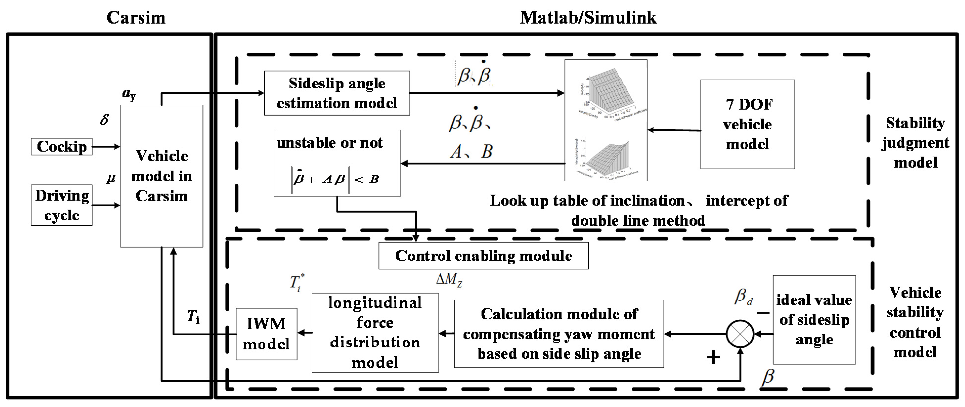
In order to assess phase planes, sideslip-angle estimation algorithm, optimal algorithm of torque distribution, and torque control method proposed in the paper, a simulation model for the stability control system of electric vehicles with four IWMs is built based on Matlab/Simulink and Carsim. The architecture for cosimulation model is presented in the Figure 5. The driver–vehicle–road model is established in Carsim. The other two models are established in Matlab/Simulink. The first is the criterion of vehicle stability model, including the estimation model of sideslip angle and 7-DOF vehicle model. The second is the vehicle stability control model, including the calculation model of yaw moment based on the sideslip angle, the wheel longitudinal forces distribution model, and the IWM model.

6.1. Vehicle Model

The advantage of using Carsim in the cosimulation model is that Carsim can provide reliable driver–vehicle–road models to ensure the accuracy of simulation. However, there is no electric vehicle with IWM model in Carsim. Therefore, in this paper, the electric vehicle model with 4 IWMs is obtains by changing the power transmission system scheme of traditional vehicle model in Carsim. The method is as follows: the power transmission system of the traditional vehicle in Carsim is changed to external components; the IWM model is built in Matlab/Simulink; and the torque output from the in-wheel-motor model is transmitted to the wheel module of Carsim.

6.2. IWM Model

Based on the research objectives, the first order time-delayed system for is selected IWM model [13]:

$$G(s)\frac{T}{\min (T^{\ast },T_{\max })}=\frac{1}{\xi \cdot s+1}$$

(30)

where T is the actual torque of motor, T* is the target torque of motor, $\xi$ is a constant determined by the motor parameters, and s is the Laplace operator. T_max is the maximum torque at the current speed. When the motor speed is lower than the base speed, T_max is a constant. When the motor speed is higher than the base speed, T_max is a function of the motor speed.

7. Simulation Evaluation

7.1. Evaluation of Sideslip-Angle Estimation

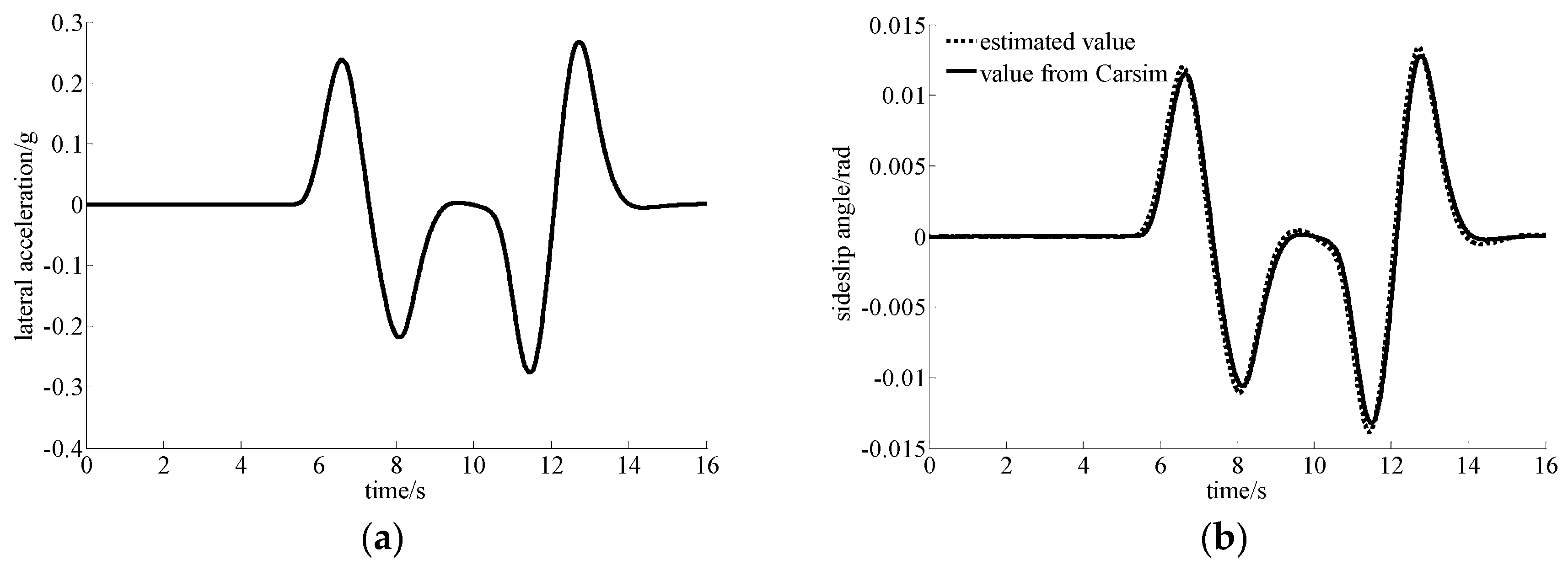
The accuracy of sideslip-angle estimation is the premise of the stability control system for an electric vehicle with four IWMs. Therefore, we assessed the accuracy of sideslip-angle estimation through several working conditions this paper, such as double-lane change maneuver, square-wave incremental steering, sinusoidal delay steering, etc. In this paper, the effect of sideslip-angle estimation is illustrated by taking double-lane change maneuvers under two velocities as examples. The road adhesion coefficient is 0.8, and the vehicle velocity is 40 km/h and 100 km/h, respectively. The simulation results are shown in Figure 6 and Figure 7.

It can be seen from Figure 6 that when the vehicle velocity is 40 km/h, the lateral acceleration of vehicle is less than 0.4 g, and the vehicle is in a stable state. The estimation of sideslip angle by the extended Kalman filter algorithm can well follow the output value of Carsim.

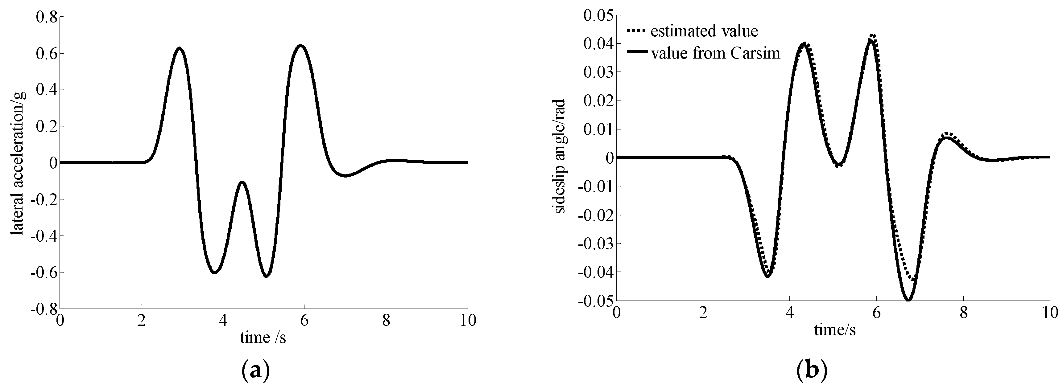
It can be known from Figure 7 that the lateral acceleration of the vehicle is more than 0.4 g when the vehicle velocity is 100 km/h, indicating that the vehicle is in an unstable state. The estimation of sideslip angle by the extended Kalman filter algorithm is slightly less than the output value of Carsim at the peak value, and other parts can follow the output value of Carsim well.

The simulation results show that the proposed estimation algorithm for sideslip angle can follow the output value of Carsim, no matter if the vehicle is stable or unstable, and can meet the requirements of stability control system of electric vehicle with four IWMs.

7.2. Evaluation of Torque Distribution

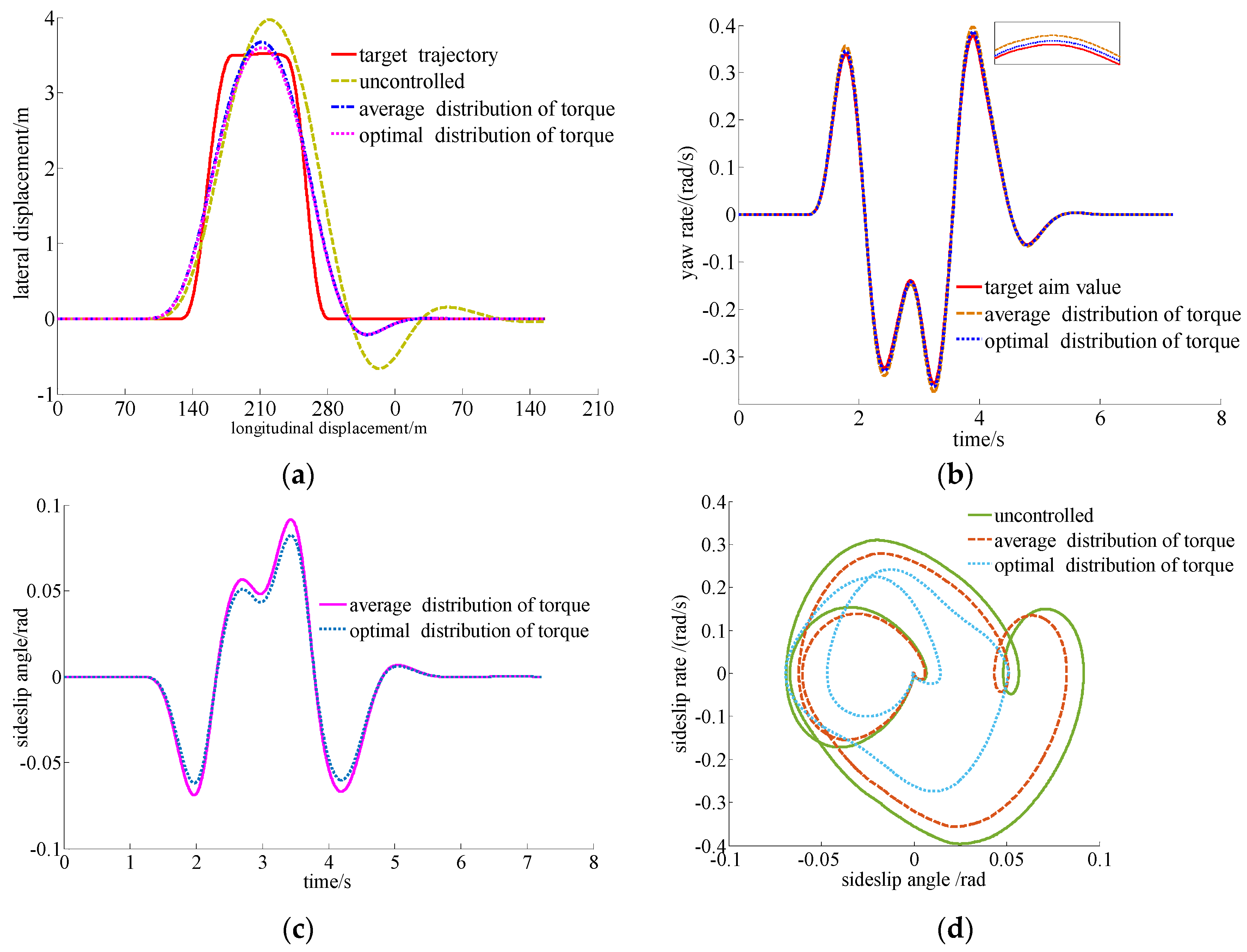
The double-lane change maneuver is used to verify the correctness of quadratic programming torque distribution. The road adhesion coefficient is 0.8, and the vehicle velocity is 130 km/h. The simulation results are as follows:

As shown in Figure 8a, vehicle trajectories without stability control have a large deviation from the target trajectories. The vehicle tends to be unstable. However, the direct yaw moment control (DYC), based on the average torque distribution and the optimal torque distribution, can make the deviation between the actual trajectories and the target trajectories smaller. As shown in Figure 8b, the DYC, based on optimal torque distribution, can make the vehicle yaw rate closer to the target value than the average distribution method. As shown in Figure 8c,d, the sideslip angle, based on optimal torque distribution method, is limited to a small range, and the $\beta -\dot{\beta }$ phase portraits return to the origin more quickly than that without control. This shows that the vehicle is more stable, and it can be known that the control effect of optimal torque distribution method is better than the average distribution method. 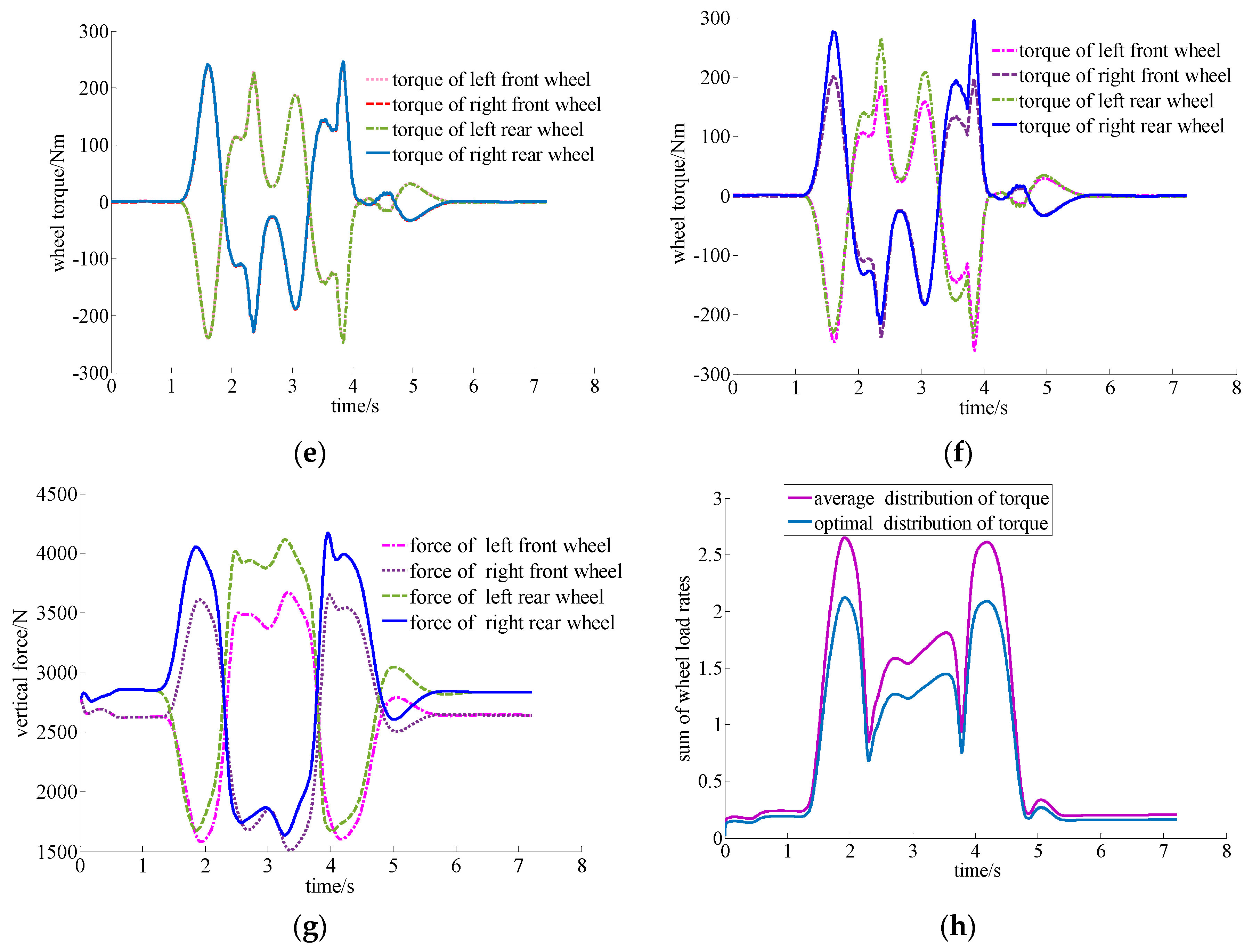As shown in Figure 8e–g, the torque value of each wheel, based on the optimal torque distribution, is consistent with trend of the wheel vertical forces. This distribution mode enables each wheel to adjust the longitudinal forces reasonably and avoid the vertical forces from reaching the longitudinal forces saturation rapidly, especially if the tire vertical force is small. As shown in Figure 8h, the sum of the wheel load rates based on the optimal torque distribution method is smaller than that of average torque distribution method. This shows that the optimal torque distribution control can make the torque distribution of each wheel more reasonable, and the adjustable margin of longitudinal forces is larger, which can make the vehicle more stable.

7.3. Evaluation of Vehicle Stability Control

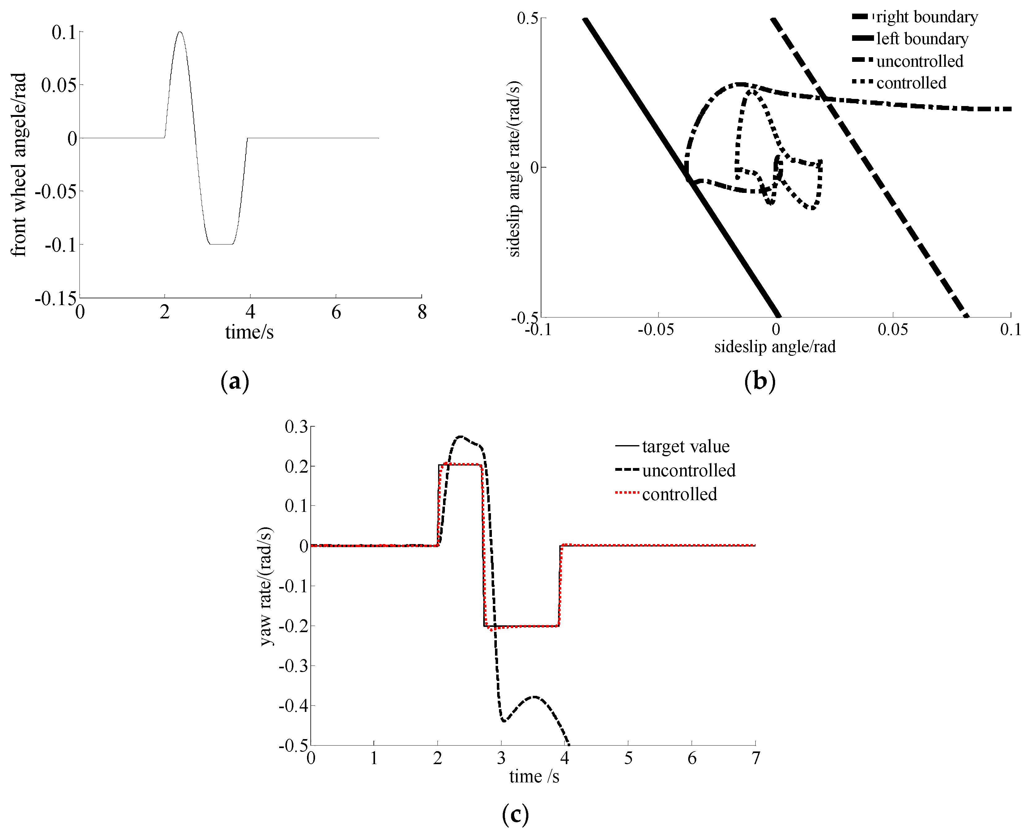
In this paper, the effectiveness of the stability control for an electric vehicle with four IWMs is verified through several working conditions, such as double-lane maneuver, square-wave incremental steering, sinusoidal delay steering, etc. A typical sinusoidal delay condition is taken as an example to illustrate it. The specific working condition is as follows: the road adhesion coefficient is 0.4, the vehicle velocity is 70 km/h, the amplitude of front wheel angle is 0.1 rad, the input frequency of front wheel angle is 0.7 Hz, and the time delay is 500 ms. The specific signal is shown in Figure 9a. As shown in Figure 9b, when the stability control is not applied, the $\beta -\dot{\beta }$ phase portraits of the vehicle exceed the stability boundary lines, and the vehicle is seriously unstable. When the stability control is applied, the $\beta -\dot{\beta }$ phase plane does not exceed two boundary lines, and the vehicle is in a stable state. It shows that the stability control system proposed in this paper is effective. In order to further illustrate the problem, the change of yaw rate is analyzed. As shown in Figure 9c, the yaw rate of the vehicle can follow the target value well when the stability control is applied. However, when the stability control is not applied, the yaw rate of the vehicle deviates from the target value seriously, and this means that the vehicle is seriously unstable.

8. Conclusions

The stability control for electric vehicles with four IWMs is the premise to give full play to its advantages that longitudinal forces of each wheel can be adjusted independently. Aiming at this key problem, the stability control system for electric vehicles with four IWMs based on the sideslip angle is studied. The following conclusions are drawn:

(1) Considering the key factors such as vehicle velocities and road adhesion coefficients, the criterion of vehicle stability based on $\beta -\dot{\beta }$ phase planes is established, and $\beta -\dot{\beta }$ phase planes are got by a 7-DOF vehicle model. On the premise of considering the velocities and accuracy of simulation, maps of inclinations and intercepts for boundary lines of $\beta -\dot{\beta }$ phase planes are established based on a large number of simulations, and it is used in the stability control system for electric vehicles with four IWMs through looking up a two-dimensional table.

(2) To solve the problem that sideslip angle is difficult to measure directly, an estimation algorithm for sideslip angle based on the extended Kalman filter is designed. Based on sliding-mode control, the DYC is proposed, together with wheel driving/braking torque distribution control method which takes the minimum sum of squares of wheel load rates as the optimization objective.

(3) Based on MATLAB/Simulink and Carsim, a cosimulation model for stability control of electric vehicles with four IWMs is built. The accuracy of $\beta -\dot{\beta }$ phase plane, estimation algorithm for sideslip angle, optimal algorithm of torque distribution, and torque control method are assessed. Relevant research can provide some references for the development of stability control system of electric vehicles with four IWMs.