Research on Automatic Parking System Strategy

Abstract

The development of the automobile industry and the increase in car ownership has brought great traffic pressures to the city, among which, the difficulty of parking has become a serious problem to the majority of drivers. An automatic parking system can help drivers to complete parking operation or automatic parking task, and a decision control system is an important part of automatic parking system. In this paper, a strategy for generating the shortest parking path based on a bidirectional breadth-first search algorithm combined with a modified Bellman–Ford algorithm is proposed for automatic parking systems. Experimental results show that this scheme can improve the performance of an automatic parking system, especially in a complex environment.

1. Introduction

Nowadays, the development of automotive technology, to some extent, represents the highest level of science and technology available. With the innovation of technology and the improvement of people’s living standards, cars have become an indispensable means of transportation for people’s daily life and travel [1,2,3]. However, the increase in the number of cars gives rise to a series of problems. As can be seen from previous reports and data, reversing accounted for 34% of all accidents worldwide in 2017 and 2018, with human factors accounting for at least 80%. The self-parking system can greatly reduce the occurrence of such accidents, and people’s attitude towards autonomous driving technology is also positive [4].

Automatic parking system approaches can be divided into two categories. The first is the path planning-based method [5,6,7,8,9], which plans the geometric reverse path of the vehicle by referring to the environmental information in the parking space and finally makes the planning and sends control commands to the actuator. The other is the method based on the experience of experts or operators [10,11,12,13]. The automatic parking system collects control information from the body information data and determines the vehicles that achieve automatic parking. The two methods can realize autonomous parking. The former has low requirements for an on-board sensor performance and easy system transplantation, which is more suitable for the use and promotion of most small cars. In view of the above, this paper discussed and designed an automatic parking system based on path planning. Automatic parking is also called automatic reversing [14]. When the car needs to park, it will first drive to the parking starting area and then start the automatic parking function without the driver’s control. Using the information collected by the sensor on the vehicle body to control the actuator with a certain control algorithm, the car can complete parking in a narrow space. As one of the key technologies in autonomous driving [15], more and more research institutions and personnel have been involved in the research.

J. Yu et al. [16] designed a set of automatic parking system fuzzy control system. Based on fuzzy control and position algorithm, the control algorithm based on ultrasonic ranging was simulated. In [17], W.X. Xie et al. applied the extraction method of fuzzy rules based on clustering effective neural network to the automatic parking system, which overcame the shortcomings of insufficient extraction of rules and the difficulty in determining the number of rules when training samples were not sufficient. Z.J. Li [18] from Jilin University adopted genetic algorithm to design fuzzy controller of automobile parking system and optimize fuzzy control. M. Lee et al. [19] proposed a method to detect parking spaces with probabilistic occupancy filter in view of the obstacle shielding problem existing in the detection of the AVM traditional sensor. Piao Changhao et al. [20] proposed a multi-sensor information integration and adaptive trajectory generation method for parking space recognition, which was robust to the non-parallel initial state of vehicles. Wang Wenjia et al. [21] proposed an automatic parking scheme based on model-free adaptive control. They only used the input data of front wheel angle and the output data of preview deviation angle generated in the process of automatic parking to expand the application scope of the method. In [22], Junzuo Li et al. proposed an automatic parking model experiment based on the deep reinforcement learning. Experiments showed that the model has good generalization ability. For path planning, researchers have explored many effective solutions based on the research of environment perception. Lozano and Wesley proposed the visualization method [23], whose most important feature is that obstacles are represented in the form of polygons or multilayers. Brooks and Lozano proposed the grid method, which decomposed the robot’s working environment into a series of simple units, adopted the four-branch tree model based on position code, and searched the path through optimization algorithm. The path search strategy adopted by this model was the traditional Dijkstra algorithm [24]. Hatti proposed the law of virtual forces. The central idea of this law was that a motion in a virtual artificial field can be thought of as a robot moving through the environment, and that any two objects had a gravitational pull, including obstacles. The acceleration of the robot is represented by the resulting force controlling the robot’s direction of motion and the computed position. However, the deadlock phenomenon [25] was very easy to occur in this situation.

To sum up, the research on automatic parking system is not perfect. It is difficult to guarantee the success rate of such automatic parking system under most complex parking conditions [26]. In recent years, many scholars have been using the improved genetic algorithms [27], the ant colony algorithms [28], and other methods to plan robot paths in intelligent algorithm research [29]. These intelligent algorithms are very effective in dealing with certain self-parking situations, but in other specific situations, the efficiency of the algorithm is reduced. In order to overcome these limitations, we design an automatic parking system, which can obtain a good parking path in a complex environment with multiple obstacles. This paper established simplified kinematics of vehicle based on the Akaman steering mechanism. We designed a path planning strategy based on rasterized map using a bidirectional breadth-first search algorithm. A modified Bellman–Ford algorithm was also designed to continue the recursive operation for the path between the source point and the target point, and update the optimized path planning results. Finally, the path was smoothed by cubic spline interpolation. In conclusion, the main contributions of this paper are as follows: (1) The simplified motion model of vehicle based on Akaman steering mechanism was studied. According to obstacles, vehicle locations and parking space coordinates, the constraint conditions in the path planning algorithm were generated. By the relative position of vehicle and parking space, the parking end condition was given. (2) Through the improvement of the Bellman–Ford algorithm, it can be integrated into the bidirectional breadth-first search algorithm to optimize the previous generated parking path, which reduced the computational burden of the program to a certain extent.

The rest of this paper is divided into four parts. The initialization program of this paper will be described in detail in Section 2. The parking path planning strategy is designed in Section 3. The experimental results and discussions are given in Section 4. In addition, the conclusion is made in Section 5.

2. The Initialization Program

2.1. Vehicle Kinematics Model

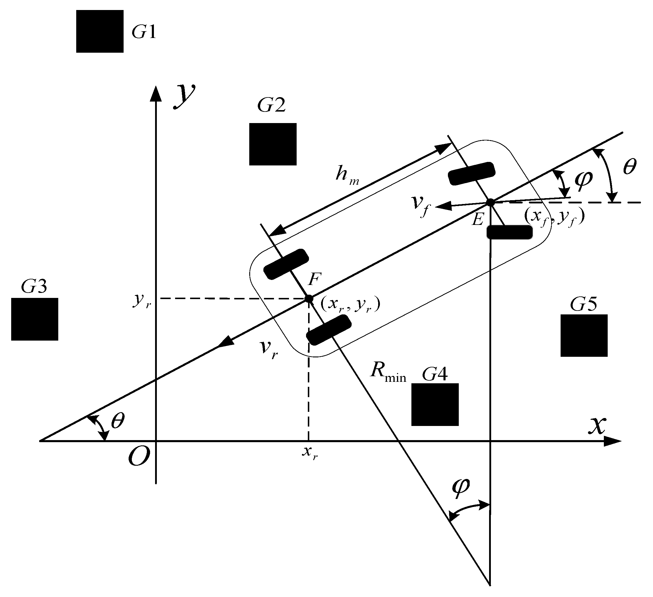
In order to establish the grid map of the model in this paper, it is necessary to establish the kinematics model of the vehicle moving at a low speed first, and demarcate the relationship between the vehicle angle and the parking process. The coordinate system of parking space is defined as $\mathrm{xoy}$, as shown in Figure 1.

From Figure 1, we can see that it is necessary to obtain the steering angle and the vehicle state before studying the parking motion. Simply, we should know the horizontal and vertical coordinates of $F$ (midpoint of rear wheel axle) and $E$ (midpoint of front wheel axle). In addition, $G1,G2,G3,G4,G5$ are obstacles, and their coordinates also need to be obtained. The coordinate of Point $F$ is $\left(x_r,y_r\right)$, and $v_r$ is the speed of the rear wheel axle. The coordinate of Point E is $\left(x_f,y_f\right)$, and $v_f$ is the speed of Point E. Let $\theta$ be the heading angle of the whole vehicle, and the motion relation of the vehicle at low speed is as follows.

$$x_r^2+{\left(y_r-h_{m}cot\phi \right)}^2={\left(h_{m}cot\phi \right)}^2$$

(1)

where $h_m$ is the wheelbase, $\phi$ is akaman angle.

According to Formula (1), Point $F$ at a low speed has nothing to do with the vehicle speed, but it is related to the Akaman angle. Therefore, it is easy to determine the trajectory of Point $E$ and the area which the vehicle moves. Given the vehicle width is $W_d$, in order to simplify the model, constraint conditions and grid map are determined according to the above model.

2.2. Kinematic Constraints

The constraint space condition can be used as the boundary judgment condition in the path planning program, which makes the path moving scheme generated by the decision system have executable meaning after decision process. We know the coordinate of E $\left(x_f,y_f\right)$ and the width of the vehicle $W_d$. From the perspective of fuzzy control, the movement process of the front and the rear wheels midpoint can be regarded as the trajectory of the vehicle. In here, coordinate set $Z=\left\{G_1\left(x_1,y_1\right),G_2\left(x_2,y_2\right),G_3\left(x_3,y_3\right)\dots G_N\left(x_n,y_n\right)\right\}$ is used to represent the center point position of obstacles, and set $L=\left\{l_1,l_2,l_3\dots l_n\right\}$ is used to represent their radius (for irregular obstacles, the maximum width is chosen as the radius). After the completion of the relevant pretreatment, when generating the grid map, the obstacles closest to the vehicle are firstly identified, and then whether these obstacles affect the current driving process is judged in turn. The judgment conditions are as follows.

$$\left\{\begin{array}{l}{d}_{Fmin}=min[\sqrt{{\left(x_1-x_f\right)}^2+{\left(y_1-y_f\right)}^2},\sqrt{{\left(x_2-x_f\right)}^2+{\left(y_2-y_f\right)}^2}\\ \dots \sqrt{{\left(x_n-x_f\right)}^2+{\left(y_n-y_f\right)}^2}],\left(x_{1\dots n},y_{1\dots n}\right)ϵZ\\ d_{Emin}=min[\sqrt{{\left(x_1-x_e\right)}^2+{\left(y_1-y_e\right)}^2},\sqrt{{\left(x_2-x_e\right)}^2+{\left(y_2-y_e\right)}^2}\\ \dots \sqrt{{\left(x_n-x_e\right)}^2+{\left(y_n-y_e\right)}^2}],\left(x_{1\dots n},y_{1\dots n}\right)ϵZ\\ k_x=\left(x_e+x_f\right)/2\\ k_v=\left(y_e+y_f\right)/2\\ d_{EFmin}=min[\sqrt{{\left(x_1-k_x\right)}^2+{\left(y_1-k_y\right)}^2},\sqrt{{\left(x_2-k_x\right)}^2+{\left(y_2-k_y\right)}^2}\\ \dots \sqrt{{\left(x_n-k_x\right)}^2+{\left(y_n-k_y\right)}^2}],\left(x_{1\dots n},y_{1\dots n}\right)ϵZ\end{array}\right.$$

(2)

Formula (2) is expressed as a circular operation in the program. After searching for the nearest obstacle, Formula (3) can judge whether this step can be carried out normally and mark it.

$$\left\{\begin{array}{c}{d}_{Emin}-l_{k1}>W_d/2,l_{k1}\in L\\ d_{Fmin}-l_{k2}>W_d/2,l_{k2}\in L\\ d_{EFmin}-l_{k3}>h_m/2,l_{k3}\in L\end{array}\right.$$

(3)

where, $l_{k1}$, $l_{k2}$ and $l_{k3}$ represent the radius of the obstacle closest to Points $F$, $E$ and the center of $EF$, respectively. If the known current coordinates are not satisfied with Formulas (2) and (3), the current moving scheme should be deleted from the path planning algorithm and a new path should be selected to ensure the safety of the vehicle in the process of movement.

2.3. Boundary Conditions

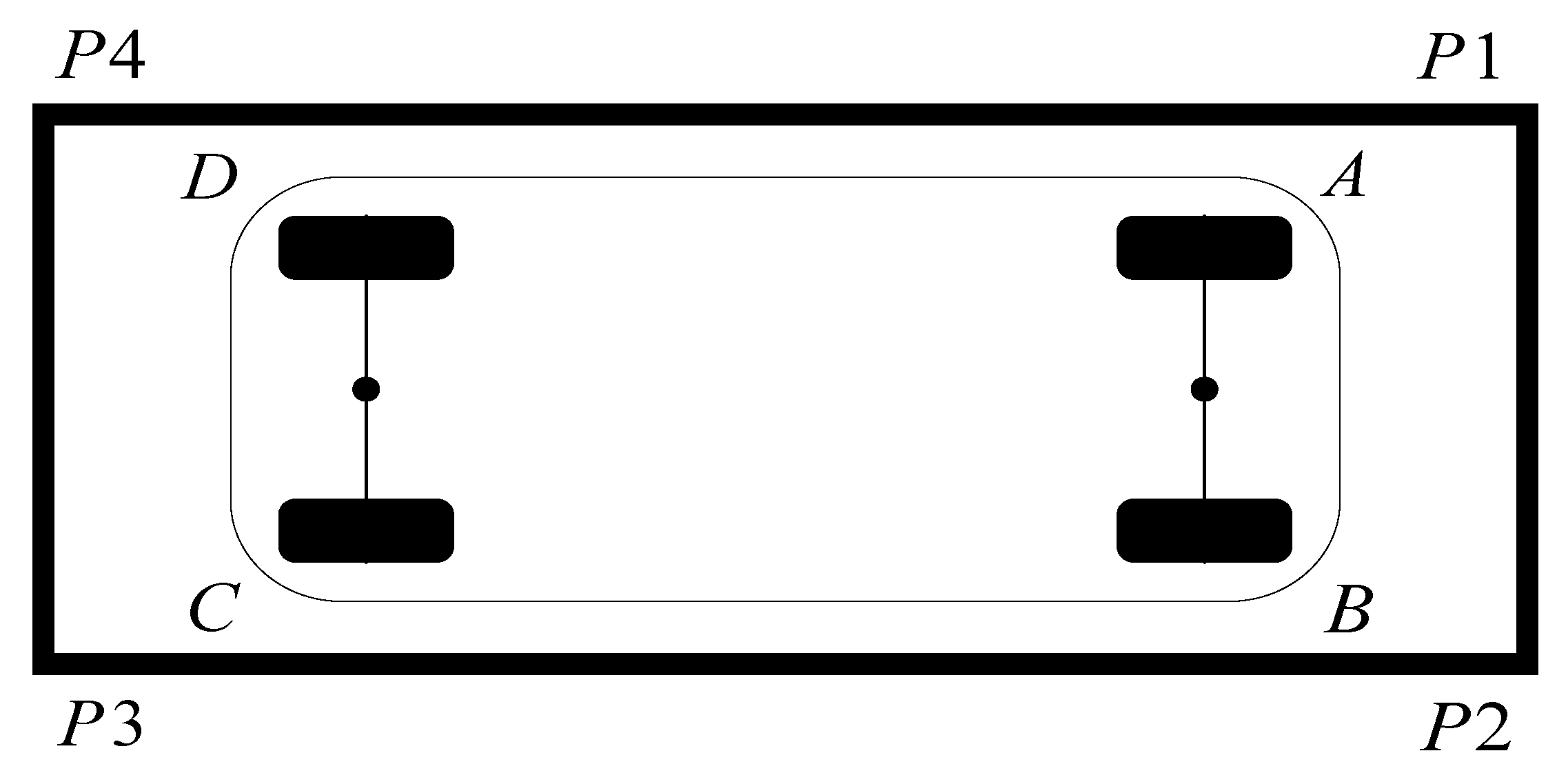
The parking system needs a judgment criterion to indicate that the vehicle has been parked. This paper assumes that the parking space is a rectangular area. In order to facilitate the algorithm adopted in this paper, the overlooking relationship between the parking space and the vehicle itself using fuzzy processing can be shown in Figure 2.

$$\left\{\begin{array}{c}{x}_r\in \left[px1\dots px4\right],y_r\in \left[py1,py2\right]\\ ax\in \left[px1\dots px4\left],by\in \right[py1\dots py2\right]\\ x_r\approx \lfloor \left|px4-px1\right|/2\rfloor \\ y_r\approx \lfloor \left|py2-py1\right|/2\rfloor \\ x_f\in \left[px3\dots px2\right],y_f\in \left[py3\dots py4\right]\\ cx\in \left[px3\dots px2\right],dx\in \left[py3\dots py4\right]\\ x_f\approx \lfloor \left|px3-px2\right|/2\rfloor \\ y_f\approx \lfloor \left|py4-py3\right|/2+h_m\rfloor \end{array}\right.$$

(4)

The four vertex coordinates of the parking space are defined as $P1\left(px1,py1\right)$, $P2\left(px2,py2\right)$, $P3\left(px3,py3\right)$ and $P4\left(px4,py4\right)$ clockwise. Conversely, the four vertex coordinates of the car are $A\left(ax,ay\right)$, $B\left(ax,by\right)$, $C\left(cx,by\right)$ and $D\left(cx,ay\right)$ clockwise. The coordinates of Points $E$ and $F$ are respectively $\left(x_f,y_f\right)$ and $\left(x_r,y_r\right)$, then the expression of parking end marker position is shown in Formula (4).

2.4. Weighted Ring Graph

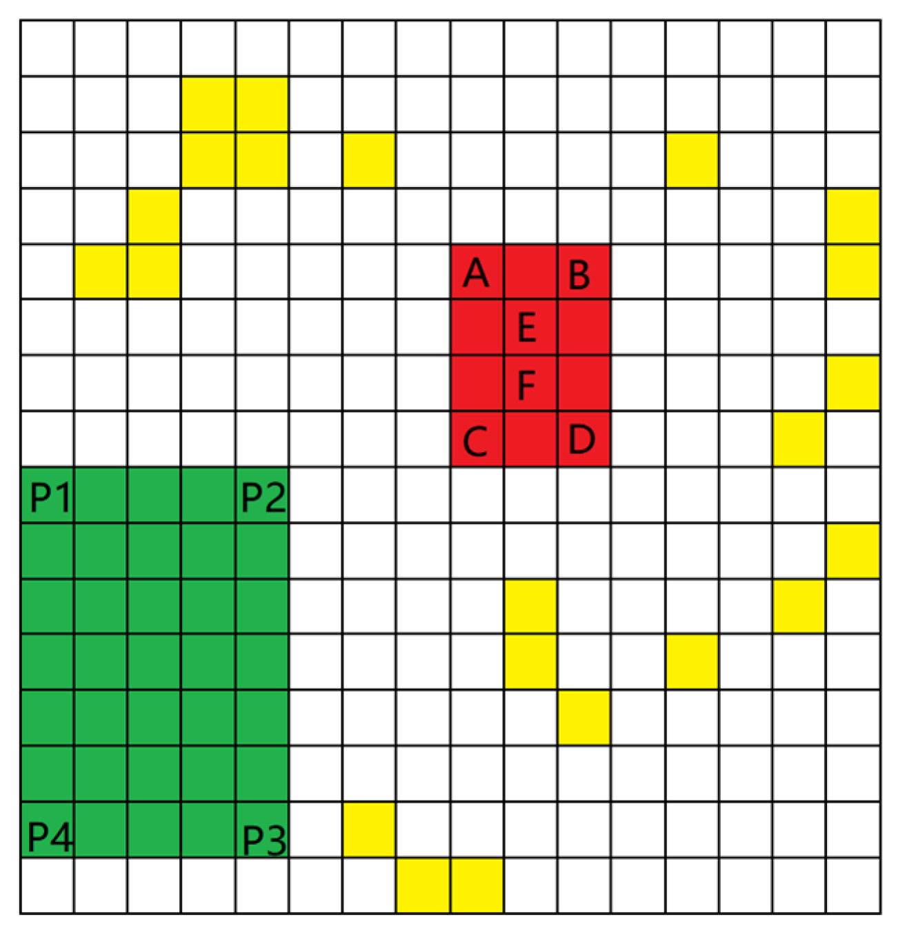
After establishing the kinematic constraints, the grid map should be built. The environment information of obstacles and garage around the vehicle is discretized according to its own factors and the environment perception system. Before the vehicle path planning, a loop diagram is needed to store the distance relationship and pass relationship between the coordinate points in the current iteration process and the coordinate points in the next decision stage. In order to facilitate the design of circular graph generation algorithm based on 2D coordinates and suitable for parking system, it is very important to generate grid map based on the established coordinate system. The grid map is shown in Figure 3.

Figure 3 abstracts the established coordinate system into relevant squares to represent the significance of this region in the whole map. For ensuring that the program can run as usual, red grids represent the location of the car, green ones represent the location of the garage, white ones represent the space for the car to drive, and yellow ones represent the obstacle. The grid size is determined by the environment awareness system and the overall performance of the vehicle’s main controller. In general, the more grids you have, the better. The content of each grid in the map generated after the garage search is determined according to the parameters of the vehicle itself and the garage information detected. Set the length of the map as $m$, width as $n$, and the first grid at the bottom left of the map as $\left(1,1\right)$. The coordinates of the four points of the garage are stored according to the size of the garage. The four points coordinates of the vehicle within that of the garage are recorded as the judgment conditions for successful parking. The whole path planning algorithm takes $E$ and $F$ as the calculation basis and takes the moving process of $F$ and the relative direction information of $F$ and $E$ as the input of iteration to analyze the path. The grid map is stored in the form of two-dimensional data. The relation of each grid to vehicles and obstacles shown in Figure 3 is expressed by Formula (5).

$$M_{ij}=\left\{\begin{array}{c}0\left(passable, white area\right)\\ 1\left(impassable, yellow area\right)\left(1\le i\le n,1\le j\le m\right)\\ 2\left(F\left(i,j\right)\right)\end{array}\right.$$

(5)

where array $M_{ij}$ is the representation of grid map, $i$ is the horizontal coordinate, $j$ is the vertical coordinate.

Defines the weighted ring diagram $G=\left(Dis,E,W\right)$ that expresses the point represented by each coordinate, where $Dis$ is the Manhattan distance from each point to another. For reducing the time complexity in the algorithm and completing the updating and searching of the shortest path, Manhattan distance representation method is used to represent the distance between points instead of Euclidean geometric distance representation method. An array of weights represents the Manhattan distance between points. Then, we use a weight array $di{s}_{ijkl}$ to describe the Manhattan distance between $\left(i,j\right)$ and $\left(k,l\right)$.

$$di{s}_{ijkl}=\left|i-k\right|+\left|j-l\right|\left(1\le i\le n,1\le j\le m,1\le k\le n,1\le l\le m\right)$$

(6)

For easy expression in the program, the weight Formula (6) is transformed into a two-dimensional array as follows.

$$Di{s}_{j+i\times {10}^{lg\lfloor j\rfloor +1},k+l\times {10}^{lg\lfloor k\rfloor +1}}=di{s}_{ijkl}$$

(7)

Set $E$ is used to represent the relation between each point and its adjacent points in the calculation process of parking path, and the initialization of this relation can be expressed as a two-dimensional array as follows.

$$E_{ijkl}=\left\{\begin{array}{c}1\{M_{ij}=0\wedge [\left(k=i-1^l=j-1\right)\vee \left(k=i+1^l=j+1\right)\\ \vee \left(k=i+1^l=j-1\right)\vee \left(k=i-1^l=j+1\right)\vee \left(k=i-1^l=j\right)\\ \vee \left(k=i^l=j-1\right)\vee \left(k=i+1^l=j\right)\vee \left(k=i-1^l=j\right)]^M_{kl}=0\}\\ 0\left(other conditions\right)\end{array}\right.$$

(8)

Let set $W$ represent the distance between the starting coordinate $F$ and each other point. To facilitate the subsequent algorithm, the weight between the source point and itself is initialized to 0. Here, $E_{x_r{y}_{r}kl}=1$ is satisfied near the source point, and $k$ and $l$ satisfy the coordinate relations in the eight adjacent regions of Point $F$, otherwise it is initialized to $\infty$. Then, in the iteration of the shortest path algorithm, the intermediate points are updated to obtain the new weights. At the same time, the set of edges between points, $E$, is also updated. Here, the initial set of weights $W$ need to satisfy Formula (9).

$$W_{ij}=\begin{array}{cc}\left\{\begin{array}{c}Di{s}_{ij}(M_{\lfloor i/{10}^{\lfloor (lg\lfloor i\rfloor +1)/2\rfloor +1}\rfloor ,i-{10}^{\lfloor (lg\lfloor i\rfloor +1)/2\rfloor +1}}=0\\ \wedge M_{\lfloor j/{10}^{\lfloor (lg\lfloor j\rfloor +1)/2\rfloor +1}\rfloor ,j-{10}^{\lfloor (lg\lfloor j\rfloor +1)/2\rfloor +1}}=0)\\ \infty (M_{\lfloor i/{10}^{\lfloor (lg\lfloor i\rfloor +1)/2\rfloor +1}\rfloor ,i-{10}^{\lfloor (lg\lfloor i\rfloor +1)/2\rfloor +1}}=1\\ \vee M_{\lfloor j/{10}^{\lfloor (lg\lfloor j\rfloor +1)/2\rfloor +1}\rfloor ,j-{10}^{\lfloor (lg\lfloor j\rfloor +1)/2\rfloor +1}}=1)\end{array}\right.& \left(i\in \left[1\dots n\left],j\in \right[1\dots m\right]\right)\end{array}$$

(9)

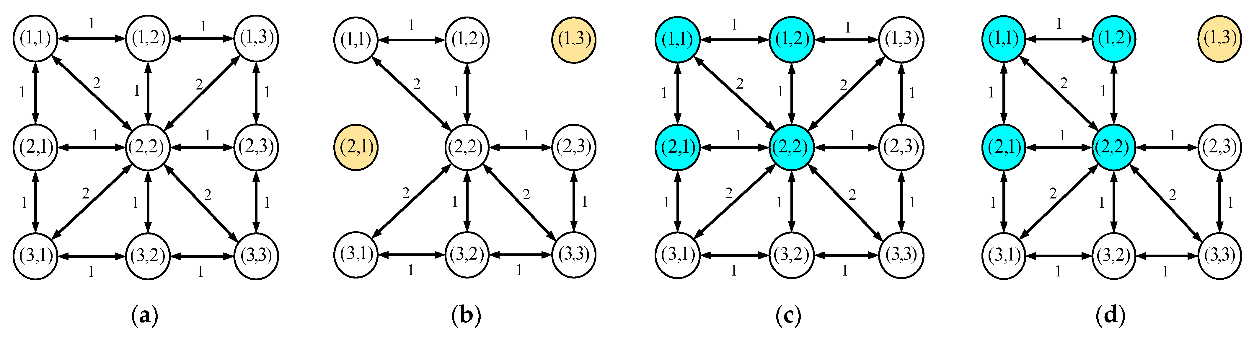
The looped graph established by Formulas (4)–(9) can be directly expressed as Figure 4. It shows a 3 × 3 straight graph representation of the whole circular graph under four conditions.

Figure 4a is the circular diagram of the barrier-free and garage-free area on normal road. The weight between any two points is one, and the diagonal Manhattan distance between the two points is two. In this area, the vehicle can move freely, and path planning can be carried out according to the shortest path scheme without making any decisions. There are obstacles in Figure 4b. In the looped graph, the type of obstacles is not considered, and only the obstacles in the area that may affect the parking process are considered. Therefore, the path planning should be carried out in the subsequent decision-making process, so as to avoid obstacles and reach the target area. There are garages in Figure 4c. When the vehicle fully enters the garage, the automatic parking is finished. Therefore, the weight between the garage and other connected normal areas is the same as Figure 4a,d belongs to the case where there are both garage and obstacles within a certain range. If the garage is connected to the grid where the obstacle is located, it is treated as in Figure 4b. Let the weight of the immediate edge adjacent to it be $\infty$, and this update will not be considered in the subsequent decision algorithm. When the map information is sent to the decision controller, and the decision controller completes the establishment of grid map and the generation of looped graph according to the map information, the initialization procedure of the decision control strategy is completed.

3. Parking Path Planning

3.1. Bidirectional Breadth-First Search Design Based on Parking Environment

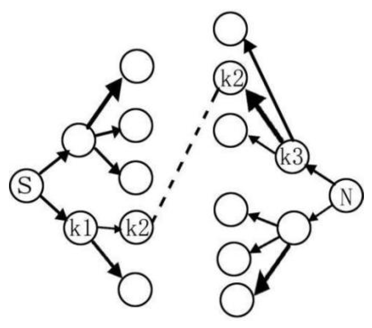
Bidirectional breadth-first search algorithm is an optimization and extension of breadth-first search algorithm. Its characteristic is that the source point and destination point start to search each other at the same time, and the algorithm ends when the two traverse to the same or several same intermediate points in the search process. Then the recursive method is used to combine the two intermediate path moving schemes to form the final overall path planning scheme. The algorithm principle diagram is shown in Figure 5.

As shown in Figure 5, the optimization scheme starts a layer-by-layer search for both the starting node and the target node at the same time. At the source Point $S$, the adjacent nodes of the layer where $\mathrm{k}1$ is located are searched first, and then the search starts from the intermediate nodes connected to each node of this layer. At the end Point $N$, we go back layer by layer from $N$. The nearest adjacent node starting with $N$ contains $\mathrm{k}3$, and each node in $\mathrm{k}3$ is searched down only with each corresponding node. When one or more nodes of two search paths overlap at a certain level, the search ends. After that, the paths of the two parts are extracted and fitted together to form the overall path.

In the structured ring graph, $G$ formed in this paper, the starting point coordinate is the coordinate of the center of the rear wheel axle, when conducting bidirectional breadth-first search. When the end point is used as a reverse search, the following processing is required. In grid map $M_{ij}$, coordinate points in the blue area can recognized as the end point coordinates as long as they meet Formula (5). In view of the special case of automatic parking, the terminal position is selected as the situation where the vehicle is parked in the middle of the garage. Set $L_{end}$ as the vertical distance from the rear axle of the vehicle to the rear of the vehicle, $\left(Ex,Ey\right)$ as the starting point of the coordinates of the reverse search, the Formula (10) is given.

$$\left\{\begin{array}{c}Ex=\lfloor \frac{px1+px3}{2}-\frac{\left(h_m+L_{end}\right)\times cos\left[arctan\left(\frac{py2-py1}{px2-px1}\right)\right]}{2}\rfloor \\ Ey=\lfloor \frac{py1+py3}{2}-\frac{\left(h_m+L_{end}\right)\times sin\left[arctan\left(\frac{py2-py1}{px2-px1}\right)\right]}{2}\rfloor \end{array}\right.$$

(10)

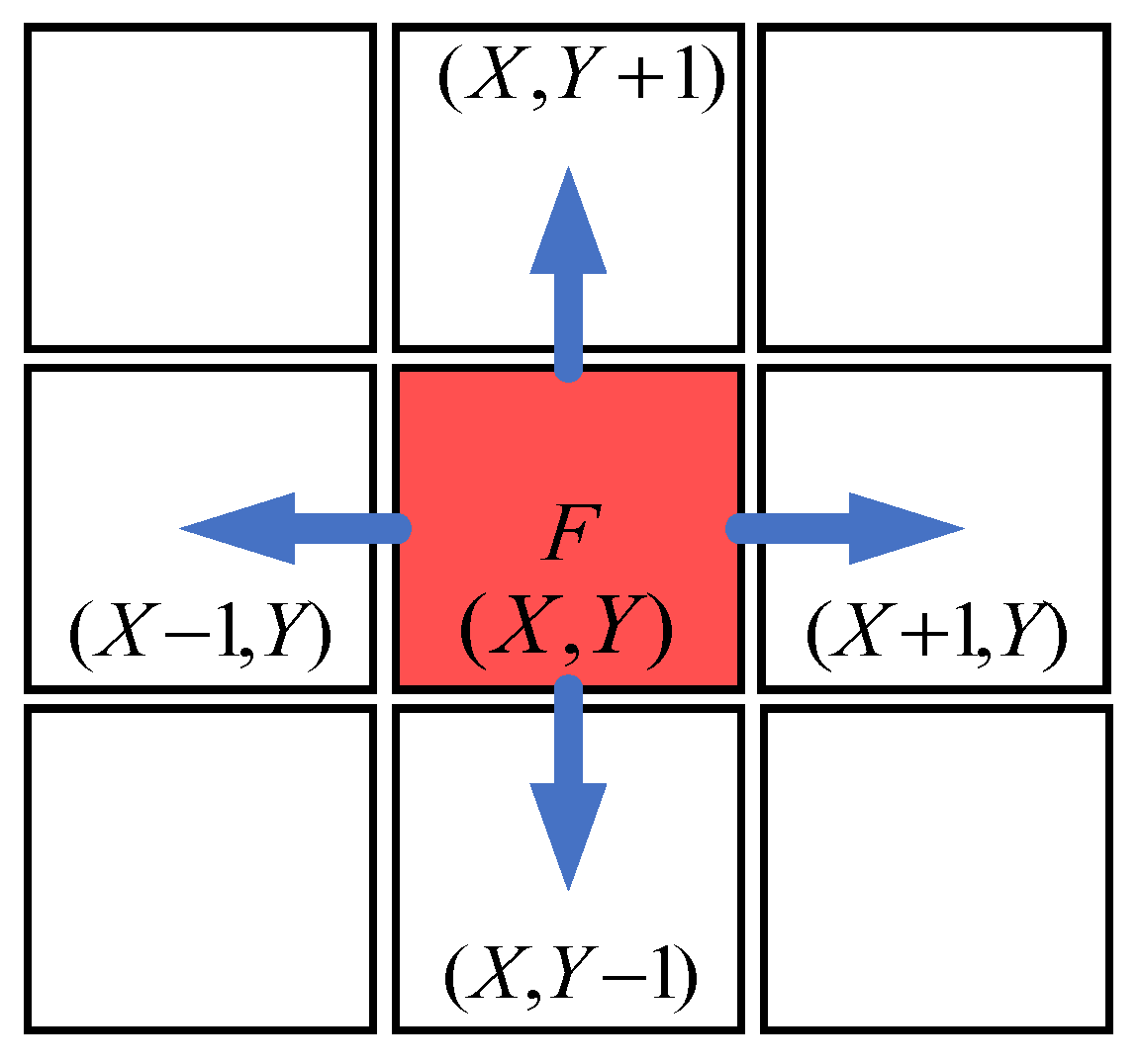
When the vehicle stops at the center of the garage, the midpoint of the line segment formed by two points $E$ and $F$ coincides with the intersection of the rectangular diagonal formed by the projection of the garage on the plane, and line $EF$ has the same slope as the edge formed by the two adjacent vertices of the projection in the coordinate system. After finishing the selection of destination, bidirectional breadth-first search is conducted for parking paths first. On the premise that vehicles can run effectively in two adjacent grids, there are four moving directions in each expansion process, as shown in Figure 6.

As shown in Figure 6, each planned path moves one grid in four directions, up, down, left, and right, as the result of path planning. Each cell move represents the car from the source point to the current total movement weight of a cumulative one, based on the iterative weighted search.

3.2. Traditional Bellman–Ford Algorithm

After determining the initial position, the Bellman–Ford algorithm fully expands this position as the source point, and finds the end point layer by layer. The intermediate point between the end point and the source point is saved in the recursive process. Let a general weighted cyclic graph as $G=\left(V,E,W\right)$, where $V$ represents the set of nodes in the graph, which is used to select the source point, intermediate point and end point in the operation of the algorithm. $E$ is the set of edges where the node is located, which is used to judge the relationship between each intermediate point and the source point or other intermediate points. $W$ represents the set of all weights between each edge and the points connected to it, which is used to update the weights from the source point to the intermediate point during the operation of the algorithm.

The algorithm steps are as follows. Let the parameter $x$ represent any intermediate point of the circle graph, and $W\left(x\right)$ represent the sum of weights from source Point S to Point $x$. At the beginning of the program, let $W\left(x\right)=\infty$, $W\left(s\right)=0$, and mark the initial length of all points other than the source point as infinity. Parameter $k$ represents the intermediate point to be judged in the iteration process. At the beginning of the program, the source point is marked first, that is, $k=s$. At this time, the dynamic transfer equation used for iteration of the algorithm is described as follows.

$$W\left(x\right)=min\left\{W\left(x\right),W\left(x\right)+d\left(k,x\right)\right\}$$

(11)

This dynamic transfer is used to determine whether the current path weight needs to be updated. Since it is solving the shortest path, the principal function in the dynamic transfer equation is the minimum. In the loop graph $G$, the weights of the points that are initially connected to the source point must be smaller than infinity, so these points will be updated directly in the first iteration. After each update, we can get $k=x$, so we keep updating down. When all the points are marked, the algorithm ends. If the destination is set to $N$, $W\left(N\right)$ represents the shortest path from source Points $S$ to $N$.

3.3. Modified Bellman–Ford Algorithm

The ownership value set $W$ is updated in the bidirectional breadth-first searched loop graph $G = \left(Dis,E,W\right)$, in which the distances from the source point to each node are preliminarily calculated. Due to this, there is no need to perform initialization operations according to SPFA algorithm standards. The modified Bellman–Ford algorithm also requires a queue to maintain its operation, so let $Qd$ be the queue used to optimize the update weight $W$. Here, an algorithm iteration completed by the bidirectional breadth-first search algorithm is regarded as the initialization operation of the improved algorithm.

The algorithm in this paper mainly adopts dynamic approximation and stores intermediate nodes and extension nodes in queue $Qd$ in a recursive way. After that, the algorithm is judged according to the characteristics of the queue. The main way to adapt to the automatic parking strategy is based on Formula (10). For this process, the weight path of grid map with Manhattan distance is proposed, and a new dynamic transfer equation is designed to complete the calculation operation of the shortest path.

After completing the improved bidirectional breadth-first search algorithm, the output path of the algorithm is stored in $Rs$ by recursive function. Let $Rs=\left\{\left(x_r,y_r\right),\left(x_2,y_2\right),\left(x_3,y_3\right)\dots \left(Ex,Ey\right)\right\}$, where the total number of steps in the path is $num$. In point set $Rs$, each data point has an array subscript, that is, the coordinates of the starting point $\left(x_r,y_r\right)$ have an array subscript of one, and the end point $\left(Ex,Ey\right)$ has an array subscript of $num$.

$$R{s}_k=\left(x_i,y_i\right)\left(1\le i\le n,1\le j\le m\right)$$

(12)

The bidirectional breadth-first search algorithm has updated the data in the weight array $W$, and the sum of the weights from many intermediate points to source points has been the local optimal solution or close to the optimal solution. Based on this situation, the dynamic transfer equation using the improved Bellman–Ford algorithm is shown in Formula (13).

$$\frac{W\left[i,j\right]=min\left\{W\left[i,j\right],W\left[i,k\right]+W\left[k,j\right]\right\},}{\begin{array}{c}W\left[i,k\right]+dis[i/{10}^{\lfloor lg\lfloor i\rfloor +1\rfloor /2}\rfloor ,i-i/{10}^{\lfloor lg\lfloor i\rfloor +1\rfloor /2}\rfloor \times {10}^{\lfloor lg\lfloor i\rfloor +1\rfloor /2},\\ k-\lfloor k/{10}^{\lfloor lg\lfloor k\rfloor +1\rfloor /2}\rfloor \times {10}^{\lfloor lg\lfloor k\rfloor +1\rfloor /2},j-\lfloor j/{10}^{\lfloor lg\lfloor j\rfloor +1\rfloor /2}\rfloor \times {10}^{\lfloor lg\lfloor j\rfloor +1\lfloor /2}]\end{array}}$$

(13)

where $W\left[i,j\right]$ represents the sum of weights from $\left(\lfloor i/{10}^{\lfloor lg\lfloor i\rfloor +1\rfloor /2}\rfloor ,i-\lfloor i/{10}^{\lfloor lg\lfloor i\rfloor +1\rfloor /2}\rfloor \times {10}^{\lfloor lg\lfloor i\rfloor +1\rfloor /2}\right)$ to $\left(\lfloor j/{10}^{\lfloor lg\lfloor j\rfloor +1\rfloor /2}\rfloor ,j-\lfloor j/{10}^{\lfloor lg\lfloor j\rfloor +1\rfloor /2}\times {10}^{\lfloor lg\lfloor j\rfloor +1\rfloor /2}\right)$. $W\left[i,k\right]+W\left[k,j\right]$ is the sum of weights between the source point and individual intermediate points after considering the process of bidirectional breadth-first search algorithm, which has a great probability to constitute the optimal path. Its purpose is to reduce the number of intermediate points in the queue, so as to avoid repeated judgment on the intermediate points that have obtained the optimal results and reduce the running time of the program.

The solution of $i$ and $j$ has been explained by Formulas (6) and (7), and $k$ in Formula (13) satisfies the following relation.

$$1\le \mathrm{k}\le \mathrm{m}+\mathrm{n}\times {10}^{\lg \lfloor \mathrm{m}\rfloor +1}$$

(14)

Formula (14) adds a new judgment selection to the traditional algorithm dynamic transfer equation. The significance is to directly apply the results of solving the shortest path between two points in the previous conclusion to solving the optimal path in the current recursive process, so as to reduce the number of intermediate points stored in the queue.

3.4. Parking Paths Smooth

The vehicle motion control problem caused by too frequent steering operation will have an impact on the parking process, so it is necessary to smooth the parking path through linear fitting for the entire grid map. In a complex environment, the car needs to be adjusted for many times in the process of parking, so there will be a situation where the reversing process and the normal movement cross each other. In this regard, after all paths fitting is completed, parking paths are required to distinguish the reversing and straight driving processes. Put parts of vehicles in the same direction together for segmented cubic spline interpolation fitting. Then, extract each section of path. Finally, according to the vehicle kinematics model, the vehicle is controlled to complete the parking process.

The cubic spline interpolation fitting function is defined as follows. In $\left[a,b\right]$, there exists $a=x_0<x_1<\cdots <x_n=b$, and a positive integer $K$ is guaranteed such that the piecewise function $s\left(x\right)$ satisfies two conditions. One condition is there are continuous derivatives up to order K − 1 in $\left[a,b\right]$. Another is there is a polynomial of degree three or less in every interval $\left[x_i,x_{i+1}\right]$. Then, the piecewise function is called a cubic spline function composed of nodes $x_0,x_1,\dots ,x_n$. The general expression for each function is as follows.

$$S_i\left(x\right)=a_i+b_{i}x+c_i{x}^2+d_i{x}^3\left(x_i\le x\le x_{i+1},1\le i\le step-1\right)$$

(15)

According to the continuity theorem at the node, Equation (16) can be obtained.

$$S_i\left(x_i\right)=y_i,S_i\left(x_{i+1}\right)=y_{i+1},i=1,2,\dots ,step-1$$

(16)

By the smoothness theorem of the first and second derivatives of the cubic spline interpolation function, Formula (17) can be obtained.

$$S_{i-1}^{\prime }\left(x_i\right)=S_i^{\prime }\left(x_i\right),S_{i-1}^{″}\left(x_i\right)=S_i\left(x_i\right),i=1,2,\dots ,step-1$$

(17)

Let $c_{step}=\frac{S_{step-1}^{″}\left(x_{step}\right)}{2}$, ${\delta }_i=x_{i+1}-x_i$, ${∆}_i=y_{i+1}-y_i$, $i=1,2,\dots ,step-1$. Substitute them into Formula (17), the following relationship can be obtained.

$$\frac{d_i=\frac{c_{i+1}-c_i}{3\times {\delta }_i}}{b_i=\frac{{∆}_i}{{\delta }_i}-c_i{\delta }_i-d_i{\delta }_i^2=\frac{{∆}_i}{{\delta }_i}-\frac{{\delta }_i}{3}\times \left(2\times c_i+c_{i+1}\right),i=1,2,\dots ,step-1}$$

(18)

To get the final solution, we need to add boundary conditions for the two endpoints. According to $2c_i=S_1^{″}\left(x_1\right)$ and $2c_{step}=S_{step}^{″}\left(x_{step}\right)$, there are three boundary conditions.

(1)

The zero-th boundary condition. The condition satisfies the relation: $c_n=0, c_1=0$.

(2)

The first boundary condition. At the endpoint, the first derivative is given, and if $S_1^{\prime }\left(x_1\right)=p_1$ and $S_{step-1}^{\prime }\left(x_{step}\right)=p_{step}$, the following relationship is satisfied.

$$\left\{\begin{array}{c}2{\delta }_1{c}_1+{\delta }_1{c}_2=3\left({∆}_1/{\delta }_1-p_1\right)\\ {\delta }_{step-1}{c}_{step-1}+2{\delta }_{step-1}{c}_{step-1}=3\left(p_{step}-{∆}_{step-1}/{\delta }_{step-1}\right)\end{array}\right.$$

(19)

(3)

The second boundary condition. For the second derivative of a given endpoint, if $S_1^{″}\left(x_1\right)=p_1$ and $S_{step-1}^{″}\left(x_{step}\right)=p_{step}$, the following relation can be deduced.

$$\left\{\begin{array}{c}2c_1=p_1\\ 2c_{step}=p_{step}\end{array}\right.$$

(20)

By combining the zero-th boundary condition and Formulas (19) and (20) into Formula (17), set $\left\{c_i\right\}$ can be solved. Then, set $\left\{d_i\right\}$ and set $\left\{b_i\right\}$ can be obtained according to Formula (18). Finally, set $\left\{a_i\right\}$ can be get according to Formula (15). In this way, the cubic spline interpolation function for each subinterval is obtained.

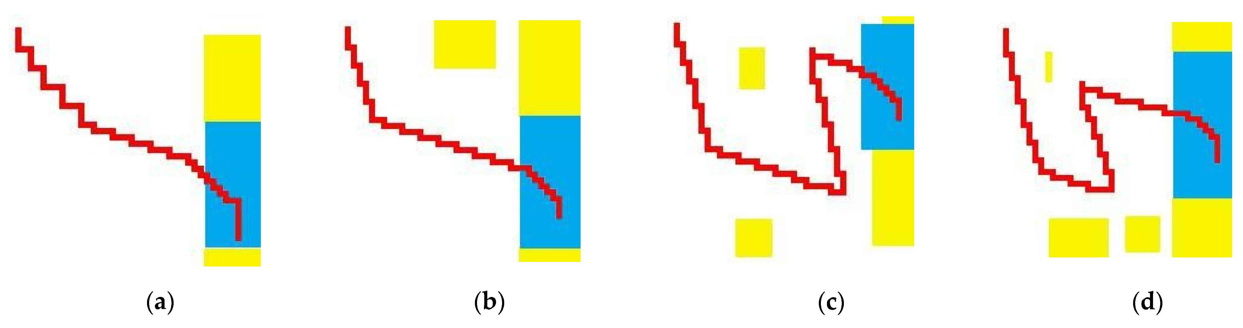
Figure 7 is a parking path diagram generated by the algorithm in this paper for several parking environments and expressed by the center point of the rear axis. The yellow area represents obstacles (obstacles do not distinguish their specific content, but only the size of the map). The blue area represents garage, and the red represents the specific path. As can be seen from (a) and (b), the two situations are relatively ideal. The vehicle goes straight in the direction of the parking space from the starting position and can directly reach the parking space without adjustment. For Figure 7c,d, there are many obstacles near the parking space, and the vehicle cannot reach the parking space in a one-time way with the traditional way. Therefore, it is necessary to adjust the parking angle according to the environmental information, so as to ensure that the car does not scratch.

4. Results and Discussion

In accordance with the relevant provisions of GA/T850 2009, urban roads, parking Spaces and lane lines were established in accordance with 1:20 to facilitate the test. Before the parking experiment based on the strategy in this paper, the parking environment must be collected first, and then the grid map must be completed. The parking experiment was conducted in a laboratory environment. The dimensions and parameters of the test vehicle are shown in

Table 1. Experimental vehicle and experimental site parameters.

	Item	Parameter
Experimental vehicle parameters	Width/Wd	17.8 cm
	Wheel base/hm	19.4 cm
	Length/L	28.5 cm
	Distance between front wheel axle and nose/Lbegin	5.4 cm
	Distance between rear axle and rear axle/Lend	2.5 cm
	Minimum turning radius/Rmin	33.28 cm
Experimental site parameters	Length/Cow	118.9 cm
	Width/Col	84.1 cm
	Number of parking Spaces available	1
	Boundary condition	One side of the parking space is shielded with a height of about 40 cm

.

4.1. Comparison of Experimental Results between Proposed Automatic Parking System and Traditional Path Planning Strategy

In this section, the proposed automatic parking system is compared with the traditional path planning strategy. Experiments are carried out under the same conditions to ensure the fairness of experimental data. The vehicle motion control system is based on the above design scheme, and the decision-making part adopts three-stage path planning scheme. Stopping speed is 3.5 km/h. The data results under three conditions are shown in

Table 2. Comparison of Experimental Results between Proposed Automatic Parking System and Traditional Path Planning Strategy.

	Traditional				Proposed
Experiment Conditions	Actual Success Rate	Ideal Success Rate	Average Vehicle Moving Time (s)	Average Algorithm Running Time (ms)	Actual Success Rate	Ideal Success Rate	Average Vehicle Moving Time (s)	Average Algorithm Running Time (ms)
Ideal conditions	86.7%	90.0%	47.3743	1.010	84.3%	100%	47.2273	7297.2
General complex conditions	60.0%	73.3%	44.7203	1.003	63.3%	90.0%	45.0593	7870.1
Extremely complex conditions	0.0%	53.3%	47.9330	1.001	23.3%	66.7%	50.2448	10,599.4

.

As shown in Table 2, under ideal environmental conditions, the actual success rate of proposed strategy is slightly lower than that of the traditional path planning method. However, as the environment becomes complicated, the success rate of the algorithm in this paper is significantly higher than that of the traditional one. On the premise of ignoring the influence of the error factors caused by vehicle kinematics on the path planning results, the success rate of the proposed strategy is much higher than that of the traditional one under ideal conditions. Under ideal conditions, the success rate of proposed strategy is 16.7% higher than that of the traditional one in general complex conditions, and 13.4% higher than that of the traditional one in extremely complex conditions. In conclusion, the higher the complexity of parking environment, the lower the success rate of the proposed path planning strategy, but the decrease is less than that of the traditional path planning method. This shows that the strategy proposed is more stable than the traditional one.

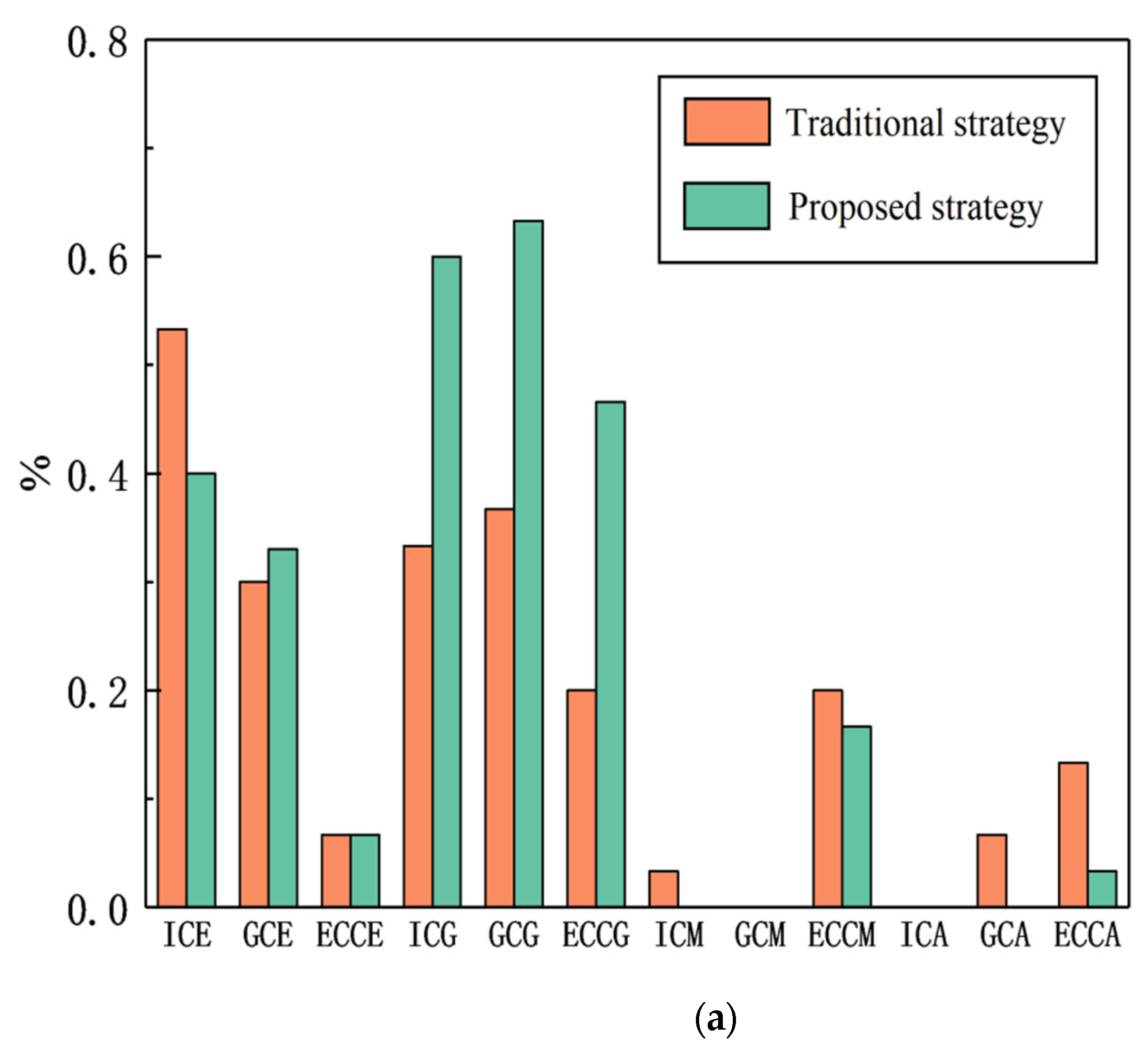
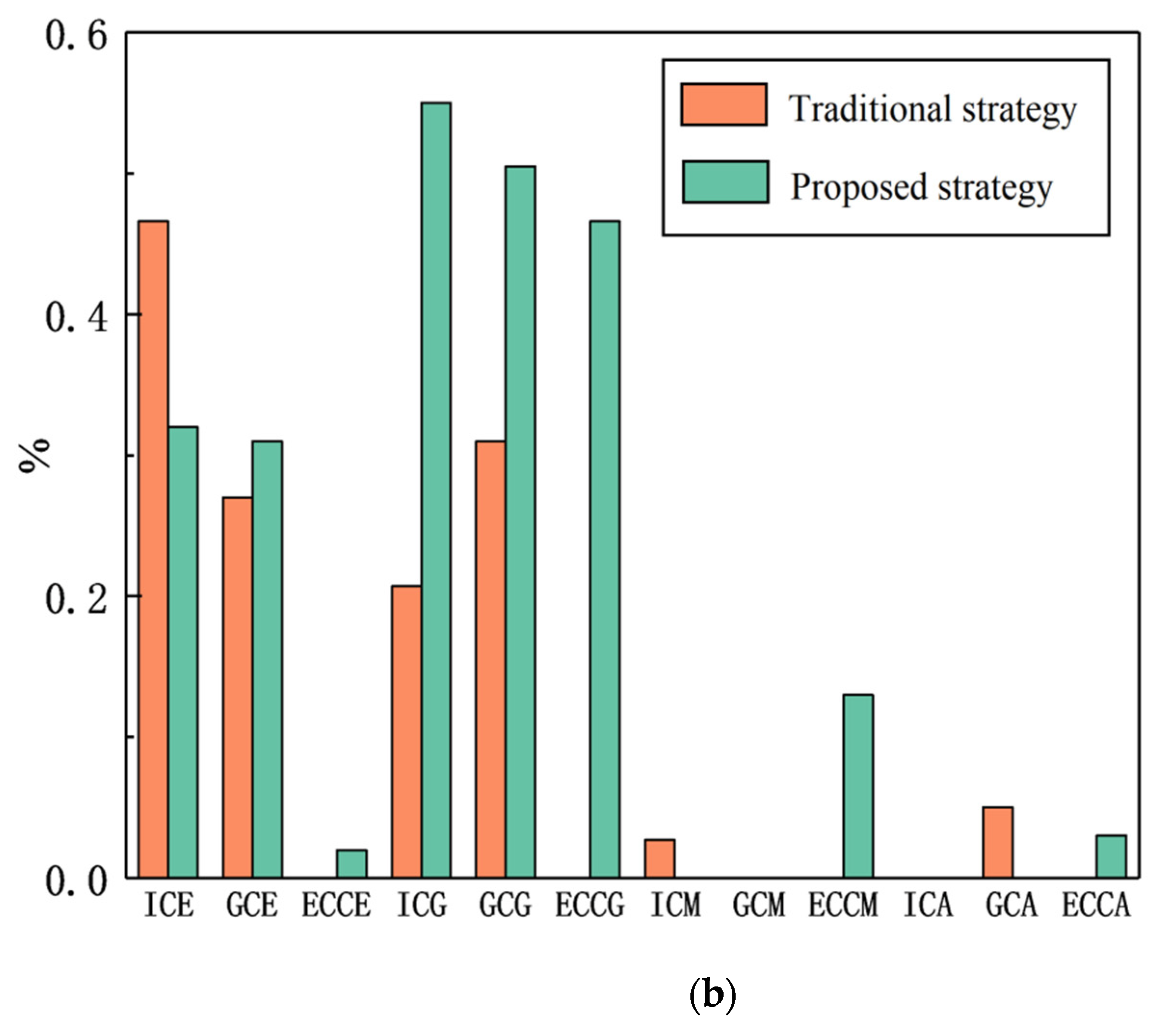
For the successful completion of automatic parking samples, their parking quality also needs to be compared. The percentages of results under different experimental conditions under actual and ideal conditions are shown in Figure 8.

From Figure 8, we can see, when parking environment in ideal condition, the quality of successful parking under traditional strategy is obviously higher than that under the strategy proposed in this paper. However, when the environment becomes more complicated, the parking effect of the strategy in this paper is better than that of the traditional parking strategy under the premise of successful parking, regardless of the ideal or actual situation. When the environment becomes particularly complex, the successful parking quality of the strategy in this paper gets more obvious. In addition, it can also be seen that no matter what state the parking environment is in, the traditional parking decision strategy tends to be good and excellent on the premise of successful parking, because it defines the moving strategy of each section and calculates the corresponding input. However, the method in this paper requires path fitting at the end, and there are many path segments calculated, so there is a certain degree of low-quality parking on the premise of successful parking. In future studies, we will focus on parking quality.

4.2. Comparison of Experimental Results between Proposed Automatic Parking System and Similar Path Planning Strategy

In this section, the comparisons between the proposed strategy and the similar method are shown in

Table 3. Comparison of the proposed strategy and the similar method in simple scenarios.

n, m	The Similar Method		The Proposed Strategy
	Step Number	Computing Time (ms)	Step Number	Computing Time (ms)
$n=80,m=40$	82	3.75	78	732.11
$n=85,m=45$	86	4.09	86	783.56
$n=90,m=40$	91	5.21	89	964.29
$n=90,m=45$	91	5.87	90	981.01
$n=95,m=50$	94	6.88	89	1035.22
$n=100,m=50$	99	7.55	92	1104.21
$n=105,m=55$	108	7.92	101	1326.89
$n=110,m=55$	113	9.69	104	1568.53
$n=120,m=60$	121	10.63	115	1925.16
$n=125,m=65$	130	12.01	120	2011.05

and

Table 4. Comparison of the proposed strategy and the similar method in complex scenarios.

n, m	The Similar Method		The Proposed Strategy
	Step Number	Computing Time (ms)	Step Number	Computing Time (ms)
$n=80,m=40$	96	5.23	91	812.25
$n=85,m=45$	105	7.86	100	901.02
$n=90,m=40$	121	8.05	119	1021.01
$n=90,m=45$	133	9.42	121	1125.69
$n=95,m=50$	145	10.21	136	1368.53
$n=100,m=50$	151	11.85	141	1685.57
$n=105,m=55$	167	12.05	157	1956.58
$n=110,m=55$	187	15.36	174	2012.55
$n=120,m=60$	192	17.69	182	2114.09
$n=125,m=65$	201	19.62	191	2456.38

. The difference of methods lies in whether the Bellman–Ford algorithm is improved. The experiment is carried out in simple and complex scenarios, with different $n$ and $m$.

Through the comparison of the similar method and the proposed strategy, it can be seen that in the case of complicated map, the improved algorithm will greatly increase the running time of the overall program, but the final path planning result will be better than that before the improvement in most cases. This is because the bidirectional breadth-first search algorithm optimizes the weights of some intermediate nodes as a whole, which greatly reduces the time and space complexity of the improved Bellman–Ford algorithm in data processing. In addition, since the automatic parking system is a slow control system and the safety is the user’s tendency and intention [30], it is acceptable to complete the path planning operation with a large time complexity before the specific vehicle movement control process.

To sum up, the characteristics of the path planning strategy in this paper can be seen. One is that when the environment is complex, the success rate is higher than that of the traditional strategy, but the parking quality after successful parking needs to be improved. Another is that while the quality of parking has improved, the total operating time has also increased significantly. Therefore, in future studies, we will also take the trade-offs between safety and speed into consideration.

5. Conclusions

In this paper, according to the characteristics of the working environment of automatic parking system, combined with different types of parking environment, an automatic parking path planning decision control system based on bidirectional breadth-first search algorithm combined with the modified Bellman–Ford algorithm was designed, which successfully overcomes the shortcomings of the existing traditional methods. Firstly, according to the characteristics of grid map, the calibration of vehicle position, obstacle and parking space was completed. Then, the motion model was studied, the motion space constraints were generated, and the parking end conditions were given according to the relative positions of vehicles and parking spaces. Finally, the Bellman–Ford algorithm was improved to integrate the bidirectional breadth-first search algorithm to optimize the previous parking path and obtain the shortest parking path. The results show that the path planning scheme designed in this paper has the characteristics of higher parking success rate than the traditional parking path planning scheme in complex parking environment, which has certain reference value for research. However, it is necessary to balance the stopping quality and speed. This will be the focus of our next phase of research.

References

- Rajamani, R.; Shladover, S.E. An experimental comparative study of autonomous and co-operative vehicle-follower control systems. Transp. Res. Part C Emerg. Technol. 2001, 9, 15–31. [Google Scholar] [CrossRef]
- Goodall, N.J. Ethical Decision Making during Automated Vehicle Crashes. Transp. Res. Rec. 2018, 2424, 58–65. [Google Scholar] [CrossRef] [Green Version]
- Thrun, S.; Montemerlo, M.; Dahlkamp, H.; Stavens, D.; Aron, A.; Diebel, J.; Fong, P.; Gale, J.; Halpenny, M.; Hoffmann, G.; et al. Stanley: The robot that won the DARPA Grand Challenge. J. Field Robot. 2006, 23, 661–692. [Google Scholar] [CrossRef]
- Lijarcio, I.; Useche, S.A.; Llamazares, J.; Montoro, L. Perceived benefits and constraints in vehicle automation: Data to assess the relationship between driver’s features and their attitudes towards autonomous vehicles. Data Brief 2019, 27, 104662. [Google Scholar] [CrossRef]
- Chen, Z.; Qiu, J.; Sheng, B.; Li, P.; Wu, E. GPSD: Generative parking spot detection using multi-clue recovery model. Vis. Comput. 2021, 37, 2657–2669. [Google Scholar] [CrossRef]
- Patil, S.; Changle, A.; Pagare, S. Automatic Car Parking System. Int. J. Adv. Res. Sci. Commun. Technol. 2021, 36, 120–123. [Google Scholar] [CrossRef]
- Sahare, S.; Moon, S.; Jaykar, S.; Shambharkar, S. Vision Based Automated Parking System. Int. J. Adv. Res. Sci. Commun. Technol. 2021, 51, 719–724. [Google Scholar] [CrossRef]
- Gao, H.; Zhu, J.; Li, X.; Kang, Y.; Su, H. Automatic Parking Control of Unmanned Vehicle Based on Switching Control Algorithm and Backstepping. IEEE/ASME Trans. Mechatron. 2020, 99, 1. [Google Scholar] [CrossRef]
- Evdokimova, T.; Sinodkin, A.; Fedosova, L.; Tyrikov, M. Algorithm for constructing a global trajectory of traffic and planning of the automatic parking route of the self-driving car. Int. J. Adv. Robot. Syst. 2020, 4, 61–67. [Google Scholar] [CrossRef]
- Chen, X.; Mai, H.; Zhang, Z.; Gu, F. A novel adaptive pseudo spectral method for the optimal control problem of automatic car parking. Asian J. Control 2021. [Google Scholar] [CrossRef]
- Zhang, J.; Li, Z.; Li, L.; Li, Y.; Dong, H. A bi-level cooperative operation approach for AGV based automated valet parking. Transp. Res. Part C Emerg. Technol. 2021, 128, 103140. [Google Scholar] [CrossRef]
- Navarro-B, J.E.; Gebert, M.; Bielig, R. On automatic extraction of on-street parking spaces using park-out events data. In Proceedings of the 2021 IEEE International Conference on Omni-Layer Intelligent Systems (COINS), Barcelona, Spain, 23–25 August 2021; pp. 1–7. [Google Scholar]
- Tirado, G.B.; Semwal, S.K. Autonomous Parking Spot Detection System for Mobile Phones using Drones and Deep Learning. In Proceedings of the WSCG “2021-29 International Conference in Central Europe on Computer Graphics, Visualization and Computer Vision” 2021, Bilson, Czechia, 17–19 May 2021; pp. 115–124. [Google Scholar]
- Yu, W.; Zhang, N.Y.; Bai, F. Fuzzy optimal control scheme for reversing problem. Mechanotronics 2001, 5, 21–24. [Google Scholar]
- Wu, J.Q.; Song, X.G. Review on key technology development of intelligent highway. J. Shandong Univ. 2020, 4, 52–69. [Google Scholar]
- Yu, J.; Jin, X. Research on automatic parking System based on Fuzzy control. Heilongjiang Sci. Technol. Inf. 2013, 85. [Google Scholar]
- Xie, W.X.; Gao, X.B. Fuzzy rule extraction method based on clustering validity neural network. J. Shenzhen Univ. 2003, 20, 14–21. [Google Scholar]
- Li, Z.J. Research on Fuzzy Control Method for Automatic Parking of Vehicles. Ph.D. Thesis, Jilin University, Changchun, China, 2016. [Google Scholar]
- Lee, M.; Kim, S.; Lim, W.; Sunwoo, M. Probabilistic Occupancy Filter for Parking Slot Marker Detection in an Autonomous Parking System Using AVM. IEEE Trans. Intell. Transp. Syst. 2018, 20, 2389–2394. [Google Scholar] [CrossRef]
- Piao, C.; Zhang, J.; Chang, K.; Li, Y.; Liu, M. Multi-Sensor Information Ensemble-Based Automatic Parking System for Vehicle Parallel/Nonparallel Initial State. Sensors 2021, 21, 2261. [Google Scholar] [CrossRef] [PubMed]
- Wang, W.J.; Hou, Z.S. Automatic parking scheme based on model-free adaptive control. Control Decis. 2021, 1001, 1–10. [Google Scholar]
- Li, J.Z.; Long, Q. An Automatic Parking Model Based on Deep Reinforcement Learning. J. Phys. Conf. Ser. 2021, 1, 1883. [Google Scholar]
- Zhang, H.W.; Huang, H.Y.; Wang, K.Y. Research status and prospect of precise movement system for military special vehicles. J. Ordnance Eng. Coll. 2017, 29, 71–74. [Google Scholar]
- Sun, Y.F.; Zhang, G. Design of automatic vertical parking system by fuzzy control based on FPGA. Mech. Des. Manuf. Eng. 2016, 45, 50–53. [Google Scholar]
- Sun, F. Research on fuzzy control strategy of automatic vertical Parking system. J. Autom. Instrum. 2016, 11, 89–90. [Google Scholar]
- Xue, L.; Leng, Y.; Lian, X. Automotive Parking Assistant Testing Scene analysis and evaluation research. J. Phys. Conf. Ser. 2021, 1, 1873. [Google Scholar] [CrossRef]
- Gao, F.; Zhang, Q.; Han, Z.; Yang, Y. Evolution test by improved genetic algorithm with application to performance limit evaluation of automatic parallel parking system. IET Intell. Transp. Syst. 2021, 15, 754–764. [Google Scholar] [CrossRef]
- Miao, C.; Chen, G.; Yan, C.; Wu, Y.Y. Path planning optimization of indoor mobile robot based on adaptive ant colony algorithm. Comput. Ind. Eng. 2021, 156, 107230. [Google Scholar] [CrossRef]
- Zhang, R.Y.; Cao, K.; Yu, S.Y.; Yu, Y. Research on generation and simulation of parking trajectory based on Spline Theory. Agric. Equip. Veh. Eng. 2014, 52, 27–31. [Google Scholar]
- Montoro, L.; Useche, S.A.; Alonso, F.; Lijarcio, I.; Bosó-Seguí, P.; Martí-Belda, A. Perceived safety and attributed value as predictors of the intention to use autonomous vehicles: A national study with Spanish drivers. Saf. Sci. 2019, 120, 865–876. [Google Scholar] [CrossRef]
Figure 1.
Create a map with a coordinate system.
Figure 2.
Vehicle and parking space diagram. and are the four boundary points of the car respectively.
Figure 3.
Grid map sketches. and are the four boundary points of the car respectively. and are the grids in the middle of the car.
Figure 4.
Schematic diagram of ring graph ring diagram based on grid map. (a) Normal; (b) obstructions; (c) garages; (d) garages and obstructions.
Figure 5.
Schematic diagram of bidirectional breadth-first search algorithm. is the source point, is the end point, and are different search layers.
Figure 6.
Diagram of four moving directions on grid map.
Figure 7.
The grid map moving path formed based on the algorithm in this paper. (a) Ideal condition; (b) traffic ahead; (c) few obstacles beside the parking space; (d) many obstacles beside the parking space.
Figure 8.
Comparison diagram of successful parking effects of the two strategies in different parking environments under actual and ideal conditions. (a) Comparison diagram of successful parking effect in different environments under ideal conditions; (b) comparison diagram of successful parking effect in different environments under actual conditions. ICE: ideal conditions (excellent); GCE: general complex conditions (excellent); ECCE: extremely complex conditions (excellent); ICG: ideal conditions (good); GCG: general complex conditions (good); ECCG: extremely complex conditions (good); ICM: ideal conditions (medium); GCM: general complex conditions (medium); ECCM: extremely complex conditions (medium); ICA: ideal conditions (average); GCA: general complex conditions (average); ECCA: extremely complex conditions (average).