2.1 Balloon data

Balloon-borne measurements of water vapor and temperature in coordination with ground-based instrumentation (lidars) started in 2014 at the Maïdo Observatory (21.08^∘ S, 55.38^∘ E) within the framework of the Global Climate Observing System (GCOS) Reference Upper-Air Network (GRUAN) (Bodeker et al., 2016). The balloon sonde payload consists of the cryogenic frost-point hygrometer (CFH) and the InterMet iMet-1-RSB radiosonde for data transmission. The iMet-1-RSB radiosonde provides measurements of pressure, temperature, relative humidity (RH) and wind data (speed and direction from which zonal and meridional winds are derived). The CFH was developed to provide highly accurate water vapor measurements in the TTL and stratosphere where the water vapor mixing ratios are extremely low (∼2 ppmv). CFH mixing ratio measurement uncertainty ranges from 5 % in the tropical lower troposphere to less than 10 % in the stratosphere (Vömel et al., 2007); a recent study shows that the uncertainty in the stratosphere can be as low as 2 %–3 % (Vömel et al., 2016). However, water vapor measurements in the stratosphere by the CFH can be contaminated by sublimation of water from an icy intake or from the balloon and payload at a pressure lower than 20 hPa (Jorge et al., 2020). The iMet-1-RSB has a temperature measurement uncertainty of 0.3 ^∘C, or 5 % in RH, with an altitude independent bias of 0.5±0.2 ^∘C (Hurst et al., 2011). As for the vertical coordinate, we use the geopotential height calculated from the iMet-1-RSB measurements of pressure, temperature and RH. Hurst et al. (2011) reported altitude-dependent differences of −0.1 to −0.2 km above 20 km between the geopotential altitudes derived from the Vaisala RS92 and InterMet iMet-1-RSB sondes. The CFH and iMet-1-RSB measurements have high vertical resolution (5–10 m) and are binned in altitude intervals of 200 m to reduce measurement noise. Here we present CFH measurements (water vapor mixing ratio and relative humidity with respect to ice, RH_ice) from two soundings performed in austral summers 2016 and 2017, when deep convection was active near Réunion Island (TS Corentin and TC Enawo; cf. Fig. 1). During austral summer, balloon launch planning is optimized using a Lagrangian forecasting tool. The 5 d backward Lagrangian trajectories initialized from the location of the Maïdo Observatory at different altitudes (9.5, 12.5, 15.5 and 18 km) are run twice a day and superimposed on current geostationary infrared satellite images to identify ongoing convection over the SWIO (http://geosur.univ-reunion.fr/foot, last access: 7 September 2020). This allows the identification of air masses with a convective origin that can be measured at the observatory, thereby maximizing local resources by only measuring when convectively influenced air masses will be sampled.

In addition to CFH measurements at the observatory, weekly Network for the Detection of Atmospheric Composition Change (NDACC) and Southern Hemisphere ADditional OZonesondes (SHADOZ) ozonesondes (Thompson et al., 2003; Witte et al., 2017) are launched from the airport (Roland Garros; 21.06^∘ S, 55.48^∘ E), located on the north side of the island (the flying distance between the Maïdo Observatory and the airport is ∼20 km). The ozonesonde is flown with a Meteomodem M10 radiosonde that provides meteorological variables such as temperature, pressure, relative humidity and winds. In this study, the NDACC/SHADOZ ozone and temperature measurements are reported in 200 m altitude bins.

2.2 Water vapor lidar data

A Raman water vapor lidar emitting at 355 nm has been operating at the Maïdo Observatory since April 2013 (Baray et al., 2013; Keckhut et al., 2015; Vérèmes et al., 2019). Laser pulses are generated by two Quanta-Ray Nd:Yag lasers, the geometry for transmitter and receiver is coaxial, and the backscattered signal is collected by a Newtonian telescope with a primary mirror of 1200 mm diameter. Raman shifted wavelengths of 387 nm (N₂) and 407 nm (H₂O) are used to retrieve the water vapor mixing ratio. Depending on the scientific investigations, specific filter points and integration times can be chosen. The raw vertical resolution is 15 m. Data are smoothed with a low-pass filter using a Blackman window. Based on the number of points used for this filter to vertically average the data, the vertical resolutions are 100–200 m in the lowest layers, 500 m in the middle troposphere, 600 m in the upper troposphere and 700–750 m in the lower stratosphere. In order to convert the backscattered radiation profiles into water vapor mixing ratio profiles, the calibration coefficient is calculated from water vapor column ancillary data: GNSS (Global Navigation Satellite System) IWV (Integrated Water Vapor). The description of the calibration method and the total uncertainty budget can be found in Vérèmes et al. (2019).

At the Maïdo Observatory, the lidar provides four to eight water vapor profiles per month. The calibrated lidar water vapor database extends from November 2013 to December 2017. The time slot of routine operations is around 19:00 to 01:00 (+1) local time, but there are intensive periods of observation during field campaigns that allow a longer measuring span. The Raman lidar water vapor observations were validated during the Maïdo ObservatoRy Gaz and Aerosols NDACC Experiment (MORGANE) intercomparison exercise in May 2015 (Vérèmes et al., 2019). During the MORGANE campaign, CFH radiosonde and Raman lidar profiles showed mean differences smaller than 9 % up to 22 km a.s.l (above sea level).

Here we used the Raman lidar measurements for 2 nights when the CFH sondes were launched at the observatory (25 January 2016 and 3 March 2017). The lidar water vapor profiles correspond to an integration time of 239 and 184 min for the nights of 25 January 2016 and 3 March 2017, respectively. The lidar water vapor profiles are interpolated to the same 200 m vertical grid used for the CFH data and are shown up to 14.5 km. The mean lidar uncertainties for the troposphere below this level are 10.5 % and 8.7 % for 25 January 2016 and 3 March 2017, respectively.

2.3 Satellite data

The brightness temperatures of the infrared (IR) channel at 10.8 µm of the geostationary weather satellite Meteosat-7 have been used to provide the regional characteristics of deep convection over the Indian Ocean. The satellite centered at 57.5^∘ E provided images for the Indian Ocean from December 2005 to March 2017.

Aura's Microwave Limb Sounder (MLS) v4.2 water vapor and ozone data were included in the study to compare with the in situ measurements and to evaluate the spatial extent of the convective air masses measured at the observatory. In particular we have used water vapor from the Stratospheric Water and OzOne Satellite Homogenized (SWOOSH) dataset (Davis et al., 2016). The SWOOSH dataset contains monthly mean stratospheric water vapor and ozone profiles from several satellite instruments for the period 1984 to present. The data are available on a 3D (latitude/longitude/pressure) grid. The SWOOSH input data for the period August 2004 to the present day correspond to measurements from the Aura MLS satellite. The MLS water vapor data are available on a pressure grid with 31 levels between 316 and 1 hPa (e.g., the vertical resolution is ranging from 1.3 to 3.6 km between 316 and 1 hPa). The estimated accuracy for MLS water vapor decreases from 20 % at 216 hPa to 4 % at 1 hPa and is ∼10 % in the TTL region (150–70 hPa).

Cloud-Aerosol Lidar with Orthogonal Polarization (CALIOP) onboard Cloud-Aerosol Lidar and Infrared Pathfinder Satellite Observation (CALIPSO) has been making backscatter measurements at 532 and 1064 nm since June 2006. We use the total attenuated backscatter coefficients ${\mathit{\beta }}_{\mathrm{532}}^{\prime }$ available from the CALIPSO V4.10 level 1 lidar data products. Following Vaughan et al. (2004), the attenuated scattering ratio SR₅₃₂ (Eq. 3 in Vaughan et al., 2004) profiles are computed as the ratio of ${\mathit{\beta }}_{\mathrm{532}}^{\prime }$ (corrected for molecular attenuation and ozone absorption) to the molecular backscatter coefficient β_m. β_m is calculated using the number density of molecules from the GEOS-5 global model of the NASA Global Modeling and Assimilation Office (GMAO) and the Rayleigh scattering cross section. More details are given in the CALIOP Algorithm Theoretical Basis Documents (ATBDs; cf. Eqs. 4.13a and 4.14).

2.4 Model

The origin of air masses measured at the Maïdo Observatory were assessed using the FLEXible PARTicle (FLEXPART) Lagrangian particle dispersion model (Stohl et al., 2005). FLEXPART is a transport model that can be run in either forward or backward mode in time. FLEXPART was driven by using ECMWF analysis (at 00:00 and 12:00 UTC) and their hourly forecast fields from the operational European Centre for Medium-Range Weather Forecasts's Integrated Forecast System (ECMWF-IFS). In March 2016, ECMWF introduced a new model cycle of the IFS into operations with a grid spacing of 9 km, roughly doubling the previous grid spacing of 16 km used since January 2010. The ECMWF model has 137 vertical model levels with a top at 0.01 hPa since June 2013. To compute the FLEXPART trajectories, the ECMWF meteorological fields were retrieved at 0.50 and 0.15^∘ and on full model levels from the Meteorological Archival and Retrieval System (MARS) server at ECMWF. The 0.50^∘ fields were used to drive the FLEXPART model over a large domain configured as a tropical channel; i.e., the domain is global in the zonal direction but bounded in the meridional direction (at latitudes ±50^∘). Furthermore, higher-resolution domains can be nested into a mother domain in a FLEXPART simulation. Thus, to have a better representation of convective transport associated with mesoscale convective systems or tropical cyclones with a horizontal dimension on the order of a couple of hundred kilometers over the SWIO, we included a nest domain covering the SWIO region (40^∘ S–10^∘ N, 20–80^∘ E). If a particle resides in the high-resolution nest, the ECMWF meteorological data at 0.15^∘ from this nest are interpolated linearly to the particle position. If not, the 0.50^∘×0.50^∘ ECMWF meteorological data from the mother domain are used to compute the trajectories. Retrieving high-resolution ECMWF fields from the MARS server for FLEXPART consists of several steps.

• Retrieve the meteorological model data output from ECMWF (horizontal winds, temperature, humidity, surface fields).

• Compute total and convective precipitation rates and sensible and latent heat fluxes from the surface.

• Calculate the vertical velocity from the continuity equation.

Therefore, the ECMWF high-resolution vertical velocity field already contains a convective mass flux component from the Tiedtke scheme used in ECMWF. The convective scheme used in the ECMWF-IFS, originally described in Tiedtke (1989), has evolved over time. Changes made include a modified entrainment formulation leading to an improved representation of the tropical variability of convection (Bechtold et al., 2008) and a modified convective available potential energy (CAPE) closure leading to a significantly improved diurnal cycle of convection (Bechtold et al., 2014). Particles are transported both by the resolved winds and parameterized sub-grid motions, including a vertical deep convection scheme. FLEXPART uses the convective parameterization by Emanuel and Zivkovic-Rothman (1999) to simulate the vertical displacement of particles due to convection. The results from model runs with and without a cumulus scheme in FLEXPART have been compared to assess whether convective mass fluxes could be resolved in the higher-resolution nest domain. The results of FLEXPART runs with and without a cumulus scheme look fairly similar (not shown), and thus here we will present only the model results with the cumulus scheme turned off.

To determine the transport history of air masses sampled by balloon launches, a so-called retroplume was calculated consisting of 10 000 back trajectory particles released from each 1 km layer of balloon launches used in this study and advected backwards in time. The initial positions of the 50 000 particles were distributed randomly within 19 vertical layers (corresponding to the MLS pressure levels between 316 and 10 hPa) with a depth of 1 km and 0.10^∘ × 0.10^∘ latitude–longitude bins centered on the balloon location. The dispersion of a retroplume backwards in time indicates the likely source regions of the air masses sampled by the in situ instruments.

3.1 Convective activity

Figure 1 shows the best tracks (i.e., a smoothed representation of the tropical cyclone's location over its lifetime; red line in each panel of Fig. 1) of tropical storm (TS) Corentin and tropical cyclone (TC) Enawo. The best track represents the best guess of the location of the tropical cyclone center every 6 h. TS Corentin started to form on 19 January 2016 east of 70^∘ E. The Meteosat-7 IR brightness temperatures on 19 January 2016 at 11:00 UTC indicate a vast clockwise circulation with some organization (not shown), indicative of tropical cyclone formation in the Southern Hemisphere. The strengthening of the northerly monsoon flow favored the deepening of the system in the subsequent days. Corentin became a moderate tropical storm (10 min maximum sustained wind speeds of 65 km h⁻¹) on 21 January 2016 at 00:00 UTC, and at that time the TS center was located at 14.93^∘ S, 75.63^∘ E, ∼2200 km to the northeast of the island. TS Corentin continued to intensify on 22 January while moving towards the south (see best track in Fig. 1). TS Corentin reached its peak intensity on 23 January at 00:00 UTC with 10 min maximum sustained wind speeds of 110 km h⁻¹ and the pressure at the center was 975 hPa. On 23 January 2016, convection was strong around 10^∘ S in the Mozambique Channel and near TS Corentin, especially in the northern part of the system. On 24 January, Corentin had weakened into a moderate tropical storm. On 25 January at 18:00 UTC (time of the balloon launch at the Maïdo Observatory), the storm was located about 2500 km southeast of Réunion Island, near 26.03^∘ S, 79.19^∘ E (Fig. 1).

Figure 1Infrared (10.8 µm) brightness temperature (K) observed by Meteosat-7 at the time of the CFH launch for 25 January 2016 at 18:00 UTC (a) and 3 March 2017 at 18:00 UTC (b). The red lines correspond to the best tracks of TS Corentin (19–31 January 2016) and TC Enawo (2–11 March 2017). The orange squares indicate the positions of the TC centers (defined as the minimum pressure in the Météo-France best track data) at the time of the satellite observation. The brown stars indicate the position of the Maïdo Observatory on Réunion Island (21.08^∘ S, 55.38^∘ E). The yellow lines correspond to CALIPSO orbit tracks on 25 January 2016 at 21:06 UTC and 3 March 2017 at 21:41 UTC. Arrows on the maps represent the wind field at 150 hPa from the ECMWF analyses at 18:00 UTC. The white contours indicate ECMWF geopotential heights at 150 hPa.

The Madden–Julian Oscillation (MJO) was active at the end of February and during the first week of March 2017 with a signal centered over Africa and the Indian Ocean. A monsoon trough was well defined all over the basin along 9^∘ S. On 28 February 2017 at 10:00 UTC, a zone of disturbed weather formed around 6.5^∘ S, 70.2^∘ E (not shown) with the building of a clockwise rotating movement inside the cloud pattern. Favored by the MJO active phase and the arrival of an equatorial Rossby wave, Enawo initially formed as a tropical disturbance on 2 March with 10 min maximum sustained wind speeds of ∼40 km h⁻¹. Enawo intensified to a moderate tropical storm at 06:00 UTC on 3 March. At the time of the balloon launch at the observatory (∼ 3 March, 18:00 UTC), Enawo was a tropical storm located near 13^∘ S, 56.42^∘ E, about 900 km north–northwest of Réunion Island (Fig. 1). It strengthened into a severe tropical storm cyclone on 5 March at 00:00 UTC and became a category 1 tropical cyclone at 12:00 UTC. TC Enawo continued to intensify while moving toward Madagascar. It became a category 4 tropical cyclone on 6 March at 18:00 UTC, with 10 min maximum sustained winds of 194 km h⁻¹. Enawo reached its peak intensity at 06:00 UTC on 7 March, with 10 min maximum sustained winds of 204 km h⁻¹ and the central pressure at 932 hPa. TC Enawo reached Madagascar's northeastern coast on 7 March at around 09:30 UTC and was the third strongest tropical cyclone on record to strike the island. After 8 March, TC Enawo gradually weakened to a tropical storm while moving southward over Madagascar.

The two balloon launches at the observatory on 25 January 2016 and 3 March 2017 were specifically planned using FLEXPART Lagrangian trajectories and Meteosat-7 infrared images. The goal was to sample the convective outflow from TS Corentin and TC Enawo, as well as convection north of Madagascar on 24 January 2016.

Figure 2Maps of convective cloud cover (gray shading) computed using 3-hourly data of Meteosat-7 infrared brightness temperature at 5 km resolution for 22–25 January 2016 (a) and 28 February–3 March 2017 (b). The red dots indicate pixels with the coldest tops (≤190 K) that capture the deepest part of convection. The dashed circle indicates a range ring of 1000 km around the Maïdo Observatory (blue star).

To assess the potential effects of deep convection in the upper troposphere and near the tropopause, we looked at the distribution of deep convective clouds in the days preceding the soundings. The location of deep convective clouds can be assessed by using maps of Meteosat-7 infrared brightness temperature. Figure 2 shows convective cloud coverage for the 3 d period preceding the sonde launch date at the Maïdo Observatory. Convective cloud coverage was estimated using 3-hourly Meteosat-7 infrared brightness temperatures at 5 km resolution. A threshold of 230 K is used to detect deep convective clouds in the Meteosat-7 brightness temperature data (i.e., pixels with brightness temperatures less than 230 K correspond to convective clouds). This threshold has been previously used to identify convection on geostationary satellite infrared images (e.g., Tissier et al., 2016). This temperature corresponds to a height of about 11 km in the NDACC/SHADOZ climatological mean summertime profile of temperature. Prior to 25 January 2016, the main deep convective activity was located ∼1500 km north of the island between 50 and 70^∘ E and around tropical storm Corentin. From 28 February to 3 March 2017, convective clouds were located ∼500 km north of the island and correspond to the intensifying tropical cyclone Enawo. The coldest cloud tops (≤190 K) that correspond to the deepest convection are indicated by red dots in Fig. 8.

3.2 Monthly mean water vapor distributions

Figure 3 show MLS water vapor volume mixing ratios at 215 and 100 hPa averaged over January 2016 and March 2017. These values were computed by averaging the SWOOSH monthly mean water vapor concentrations gridded on a regular pressure/latitude/longitude (a resolution of 5^∘ × 20^∘) grid.

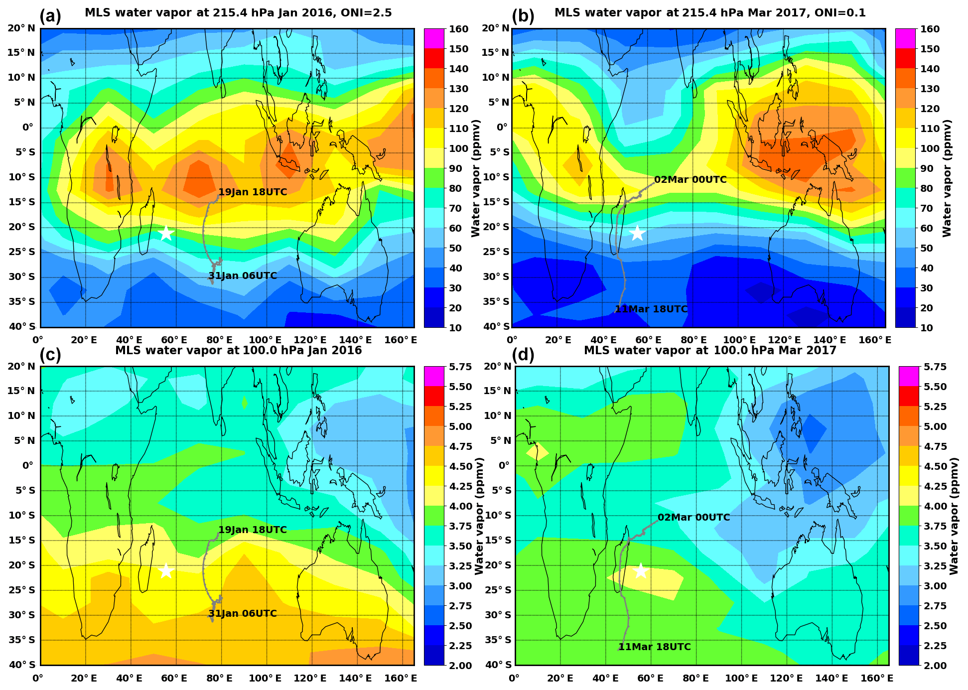
Figure 3MLS water vapor mixing ratios (ppmv) gridded in the SWOOSH dataset at 215 hPa for January 2016 (a) and for March 2017 (b). The gray lines correspond to the best tracks of TS Corentin (19–31 January 2016) and TC Enawo (2–11 March 2017). (c, d) Same as (a) and (b) but for 100 hPa.

When comparing the water vapor mixing ratio at 215 hPa in January 2016 to the one observed in March 2017, one can see that the upper troposphere over the SWIO was much moister in January 2016 than in March 2017 with three distinct regions of enhanced water vapor over central Africa, the Indian Ocean and the Maritime Continent. The mean water vapor mixing ratio at 215 hPa over the SWIO in January 2016 is greater by ∼23 ppmv compared to March 2017. Interannual variability modes such as the El Niño–Southern Oscillation (ENSO) can affect the TTL temperature and thus water vapor distribution. The NOAA Climate Prediction Center Ocean Niño Index (ONI), which is based on sea surface temperature anomalies in the Niño 3.4 region, was equal to +2.5 K in January 2016 versus +0.1 K in March 2017 (http://origin.cpc.ncep.noaa.gov/products/analysis_monitoring/ensostuff/ONI_v5.php, last access: 7 September 2020). January 2016 corresponded to strong El Niño conditions (one of the strongest El Niño events since 1950 according to the ONI index), while March 2017 was associated with neutral ENSO conditions. The water vapor mixing ratios at 215 hPa for January 2016 are in agreement with MLS December–March (DJFM) climatological values of water vapor at 215 hPa for El Niño conditions (not shown). Overall, during El Niño conditions, water vapor mixing ratios at 215 hPa are enhanced over the SWIO west of 80^∘ E. Ho et al. (2006) have studied the variations of TC activity in the southern Indian Ocean in relation to ENSO effects. During El Niño periods, TC genesis was shifted westward, enhancing the formation west of 75^∘ E and reducing it east of 75^∘ E. Therefore, on January 2016, the peak of water vapor west of 80^∘ E at 215 hPa may be related to an increase in convection associated with strong El Niño conditions.

The quasi-biennial oscillation (QBO) also affects TTL temperatures and humidity (e.g., Zhou et al., 2001; Yuan et al., 2014; Davis et al., 2013). Following Davis et al. (2013), we defined a QBO index as the zonal mean (10^∘ S–10^∘ N) of the difference in the ERA-Interim zonal wind at 70 and 100 hPa. A positive QBO index (u_70 hPa–u_100 hPa>0) corresponds to westerly shear conditions and the warm phase of the QBO (Baldwin et al., 2001). A negative QBO index corresponds to easterly shear conditions and the cold phase of the QBO (CPT temperatures are cooler during the easterly shear phase of the QBO). The mean January 2016 water vapor mixing ratio at 100 hPa over the SWIO is 4.2 ppmv versus 3.7 ppmv in March 2017 compared to the climatological values of 3.51 ppmv for January and 3.44 ppmv from March. The difference of 0.50 ppmv between the two periods cannot be explained by the phase of the QBO as both months corresponded to QBO westerly shear conditions (2.33 m s⁻¹ for January 2016 and 4.79 m s⁻¹ for March 2017). However, the higher water vapor mixing ratio at 100 hPa in January 2016 could be related to strong El Niño conditions as Avery et al. (2017) have reported large lower stratospheric (82 hPa) water vapor anomalies ($\sim +\mathrm{0.9}$ ppmv) associated with the strong 2015/2016 El Niño. The highest SWOOSH water vapor mixing ratio anomalies of $\sim +\mathrm{1}$ ppmv were observed over the Indian Ocean in December 2015 (not shown). In January 2016, the anomalies over the SWIO had eased to 0.7 ppmv (not shown).

4.1 Water vapor/ozone profiles

Figure 4 shows two CFH water vapor mixing ratio profiles (black lines) taken at the Maïdo Observatory on 25 January 2016 at 17:50 UTC and 3 March 2017 at 18:00 UTC. The lidar water vapor profiles for those 2 nights are also displayed in green. The red and purple lines correspond to NDACC/SHADOZ ozonesonde balloon profiles launched from Roland Garros airport on 18 January 2016 (purple line), 4 February 2016 (red line) and 3 March 2017 (purple line in panel b). The ozonesonde data correspond to daytime measurements (balloon launches at ∼ 11:00 UTC), while the CFH water vapor data correspond to nighttime measurements in order to coincide with water vapor lidar measurements at the Maïdo Observatory. Overall good agreement is seen between the lidar and CFH water vapor profiles over the whole troposphere. Note that the CFH water vapor profiles were not used to calibrate the lidar water vapor profiles as explained in Sect. 2.2.

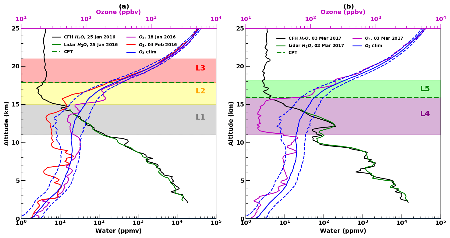
Figure 4Vertical profiles of (a) CFH and lidar water vapor profiles (ppmv) on 25 January 2016 (black and green line, respectively) and NDACC/SHADOZ ozone profiles on 18 January 2016 (purple line) and 4 February 2016 (red line); (b) CFH and lidar water vapor profiles (black and green line  respectively) and NDACC/SHADOZ ozone profile (purple line) on 3 March 2017. The location of the cold point tropopause is indicated by the dashed green line. Also shown in each plot is the 1998–2017 climatological mean ozone profile (blue line) for DJFM and the ± 1 standard deviation of the climatology corresponds to the dashed blue line The most important layers in the water vapor/ozone profiles are shaded and named.

Download

The altitude range of 2–12 km on 25 January 2016 is moister by ∼50 % than the same altitude range on 3 March 2017 (mean water vapor mixing ratio of 5076 and 4375 ppmv between 2 and 12 km on 25 January 2016 for the CFH and lidar, respectively, versus 3335 and 3398 ppmv on 3 March 2017 for the CFH and lidar, respectively). The austral summer season, with warmer temperatures and greater cloudiness, reaches its peak in January/February, and this could explain in part the higher humidity observed in January than March. In addition, January 2016 corresponded to a strong El Niño period, and this could lead to higher tropospheric moistening associated with ENSO (Tian et al., 2019). On 3 March 2017, a moist layer was observed between ∼12 and 16 km in both CFH and lidar water vapor profiles with corresponding low ozone values (Fig. 4b). On 25 January 2016, two local moist layers around 10 and 15 km associated with low ozone were observed. The lidar smoothes out the peak of water vapor at 10 km observed on 25 January 2016, but this could be due to the longer integration time used for that night (239 min). The CFH water vapor mixing ratio profiles have a minimum of 2.5 ppmv at 17.10 km (94 hPa) and 2.70 ppmv at 18.10 km (77.1 hPa) on 25 January 2016 and 3 March 2017, respectively.

Also shown is the climatological mean ozone profile for DJFM 1998–2017 (blue lines in Fig. 4). Anomalously low mixing ratios approaching surface values are seen in the upper troposphere for both the 4 February 2016 (red line in Fig. 4a) and 3 March 2017 (purple line in Fig. 4b) ozone sonde flights. In the upper troposphere, the climatological mean ozone mixing ratios range from about 60 ppbv at 10 km to 100 ppbv at 15 km. There is a steep gradient above 17 km, indicating the transition from the troposphere to the stratosphere. On 3 March 2017, ozone mixing ratios between 10 and 15 km are ∼45 ppbv below the climatological values (mean value of 25.10 ppbv for the 10–15 km layer on 3 March 2017 versus 70.1 ppbv for the climatological ozone profile).

Between 18 January and 4 February 2016, ozone mixing ratios in the upper troposphere decreased by ∼30 ppbv and are 38 ppbv below the climatological values on 4 February 2016. Tropical storm Corentin reached its peak intensity on 23 January 2016 at 00:00 UTC, and its center was located 1735 km east of Réunion Island. These low ozone mixing ratios in the upper troposphere on 4 February 2016 were observed after the storm had had its major influence on the UT ozone, transporting air with surface ozone values upward via strong convection and mixing out into the larger environment. In comparison, the 18 January 2016 ozone profile was not influenced by TS Corentin. The lower ozone values on 3 March 2017 compared to those observed on 4 February 2016 could be explained by the fact that TC Enawo was closer to the island (∼902 km north of the island), was still intensifying and was a stronger system than TS Corentin. Above ∼17 km, the ozone profiles in January/February 2016 and March 2017 are more similar to the climatological mean ozone profile, suggesting that deep convection did influence the upper troposphere but not the lower stratosphere. We will later show using FLEXPART that the moist and low ozone layers in Fig. 4 are associated with the convective outflow of a mesoscale convective system north of Madagascar on 23 January 2016.

4.2 Relative humidity and temperature profiles

Figure 5 shows the CFH profiles of RH_ice, computed using the Goff–Gratch equation (Goff and Gratch, 1946) for water vapor pressure, on 25 January 2016 and 3 March 2017, as well as collocated CALIOP nighttime backscatter measurements. The CALIOP measurements shown in Fig. 5 include only those within ±5^∘ latitude and ±10^∘ longitude of the Maïdo Observatory. The CALIOP measurements on 25 January 2016 correspond to a CALIPSO overpass east of the island around 4 h after the balloon launch, and the mean longitude difference between the CALIPSO overpass and the Maïdo Observatory is 2.4^∘ for Fig. 5a and b. On 3 March 2017, the CALIPSO overpass was west of the island and also 4 h after the balloon launch. The mean longitude difference between the CALIPSO overpass and the Maïdo Observatory is 5.3^∘. The latitude–height cross section of CALIOP SR₅₃₂ in Fig. 5 corresponds to measurements with a 60 m vertical resolution. The horizontal interval of the CALIOP data along its orbit is 330 m; for this study we use a 9-point running average to reduce noise.

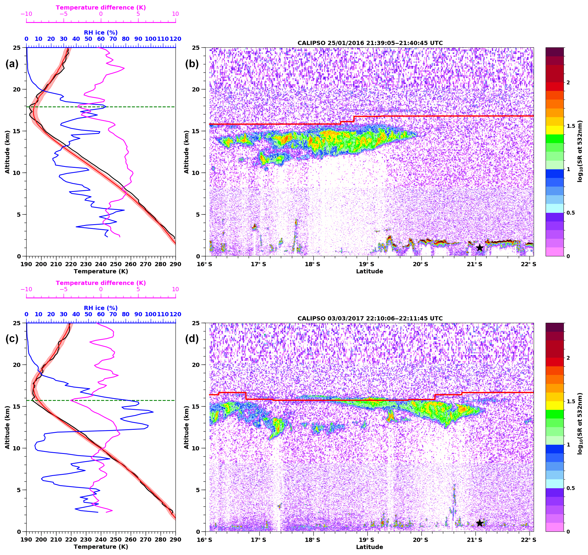
Figure 5(a, c) Vertical profiles of temperature and relative humidity with respect to ice (black and blue line, respectively) measured on 25 January 2016 at 17:52 UTC and 3 March 2017 at 18:00 UTC. The dashed green line corresponds to the cold point tropopause. The NDACC/SHADOZ climatological mean summertime (DJFM) profile of temperature (red line), the ± 1 standard deviation (red shading) and temperature anomaly (magenta line) are also shown. (b, d) Latitude–altitude distribution of CALIOP backscattering ratio at 532 nm along CALIOP track near Réunion Island on 25 January 2016 (b) and 3 March 2017 (d). The mean longitude difference between the CFH profile and the CALIOP track is 2.4^∘ on 25 January 2016 and 5.3^∘ on 3 March 2017. The red curve on each CALIOP plot corresponds to the tropopause height provided by the GEOS-5 global model data available in the CALIPSO level 1 data files. The latitude of the Maïdo Observatory is indicated by the black star on each CALIOP plot.

Download

Figure 5a and b show significant structure in the RH_ice profile measured on 25 January 2016. Higher values of RH_ice (>40 %) between 13 and 15 km coincide with higher values of CALIOP SR₅₃₂ between 12 and 15 km. The RH_ice reaches its maximum value at the cold point altitude (17.3 km). The CALIOP SR₅₃₂ indicates a cirrus cloud between ∼12 and 15 km north of the island. The cirrus layer extends from ∼16.2 to 20^∘ S corresponding to a horizontal scale of ∼ 400 km. Meteosat-7 infrared brightness temperature at 21:30 UTC, so ∼10 min before the CALIPSO overpass at 21:39 UTC in Fig. 5a and b, indicates a large area of deep convection near 15^∘ S and extending from ∼50 to 75^∘ E (not shown). The monsoon trough was located between 17^∘ S, 50^∘ E and 14^∘ S, 70^∘ E on 25 January 2016, which promoted deep convection, and convective activity was also observed in the southeastern quadrant of TS Corentin. The cirrus cloud observed below 15 km in Fig. 5a and b was most likely from convective detrainment north of Réunion Island. The RH_ice profile on 25 January indicates intertwined layers of dry air (RH_ice less than 40 %) at 7, 9, 12 and 16 km and less dry air (RH_ice∼50 %) at 8, 11, 15 and 17 km. While convection north of Réunion Island around 15^∘ S and TS Corentin had mixed the troposphere over the southwest Indian Ocean, no cirrus clouds were directly observed on 25 January 2016 above the Maïdo Observatory. The layers of RH_ice∼50 % at 15 and 17 km may be due to convective detrainment. The cirrus cloud below 15 km detected by CALIPSO north of the island on 25 January indicates that deep convection detrained ice and water vapor in the upper troposphere north of the island. There was a northerly wind between 10 and 17 km on 25 January 2016 with a peak around 25 m s⁻¹ at 15 km (cf. Fig. 1). Moist air detrained by deep convection north of Réunion near 15^∘ S may have been transported to Réunion Island in ∼6 h, and during that time the moist air mass could have mixed with drier air, thereby explaining the layers of RH_ice∼50 % at 15 and 17 km in Fig. 5. The origin of these layers has also been determined using the FLEXPART Lagrangian model, and the results are presented in the next section.

On 3 March 2017, a layer close to saturation (RH_ice>80 %) can be observed between 12 and 16 km (Fig. 5c) with RH_ice up to ∼100 % at 12.5 and 14 km below the cold point altitude (16.1 km). The altitude range 12–15.5 km corresponds to cloudy air, and a cirrus cloud can be seen in the CALIOP measurements of SR₅₃₂ between ∼13 and 15 km extending from 18.4 to 21.2^∘ S (Fig. 6d). Above Réunion Island, the cirrus is ∼1.5 km thick and the maximum thickness of ∼3 km is observed north of the island at 20.5^∘ S. A second cirrus cloud can also be observed below 15 km north of 17.4^∘ S.

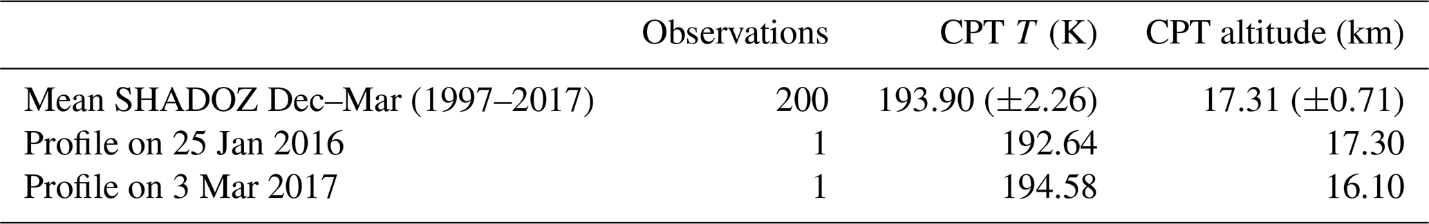
The CPT height is 16.10 km on 3 March 2017, while it is 1.2 km higher on 25 January 2016 (Fig. 5). The CPT temperature was 192.64 K on 25 January 2016 and 194.58 K on 3 March 2017. On 3 March 2017, the layer between 16 and 18 km was almost isothermal with a mean temperature of 195 K, while the tropopause was sharper on 25 January 2016.

4.3 Lagrangian analysis

The convective origin of air masses sampled in the upper troposphere and near the tropopause during the passage of TS Corentin and TC Enawo is evaluated using the FLEXPART Lagrangian model. Figure 6 presents the origins of air masses sampled within layer L1 (12.1–13.1 km, ∼178 hPa) and layer L2 (16.3–17.3 km, ∼100 hPa), which are altitudes that correspond to RHi peaks in Fig. 5 on 25 January 2016 above the Maïdo Observatory. The origins and pathways of these air masses were examined by computing 10 d FLEXPART back trajectories. In Fig. 6, the origins of air masses measured in the upper troposphere (layer L1) and near the tropopause (layer L2) are shown for 2 d and 3 d prior to the launch. The position of each air mass is depicted by 10 000 dots color coded by their altitude and is overlaid over Meteosat-7 infrared images valid at the time of the back trajectories. For example, trajectories that were originally in the lower troposphere (below 5 km) and middle troposphere (between 5 and 10 km) 2–3 d before are indicated by orange and brown dots, respectively. In other words, these air masses were transported from the troposphere to the upper troposphere/tropopause region in 2 or 3 d before being sampled by the CFH instrument on 25 January 2016 around 18:30 UTC above the Maïdo Observatory. The air mass fractions for different altitude ranges are also indicated in Fig. 6c and d. Variations in the air mass fractions over time (e.g., from the lower troposphere below 5 km) can be interpreted in terms of changes in the vertical transport due to convection over the SWIO.

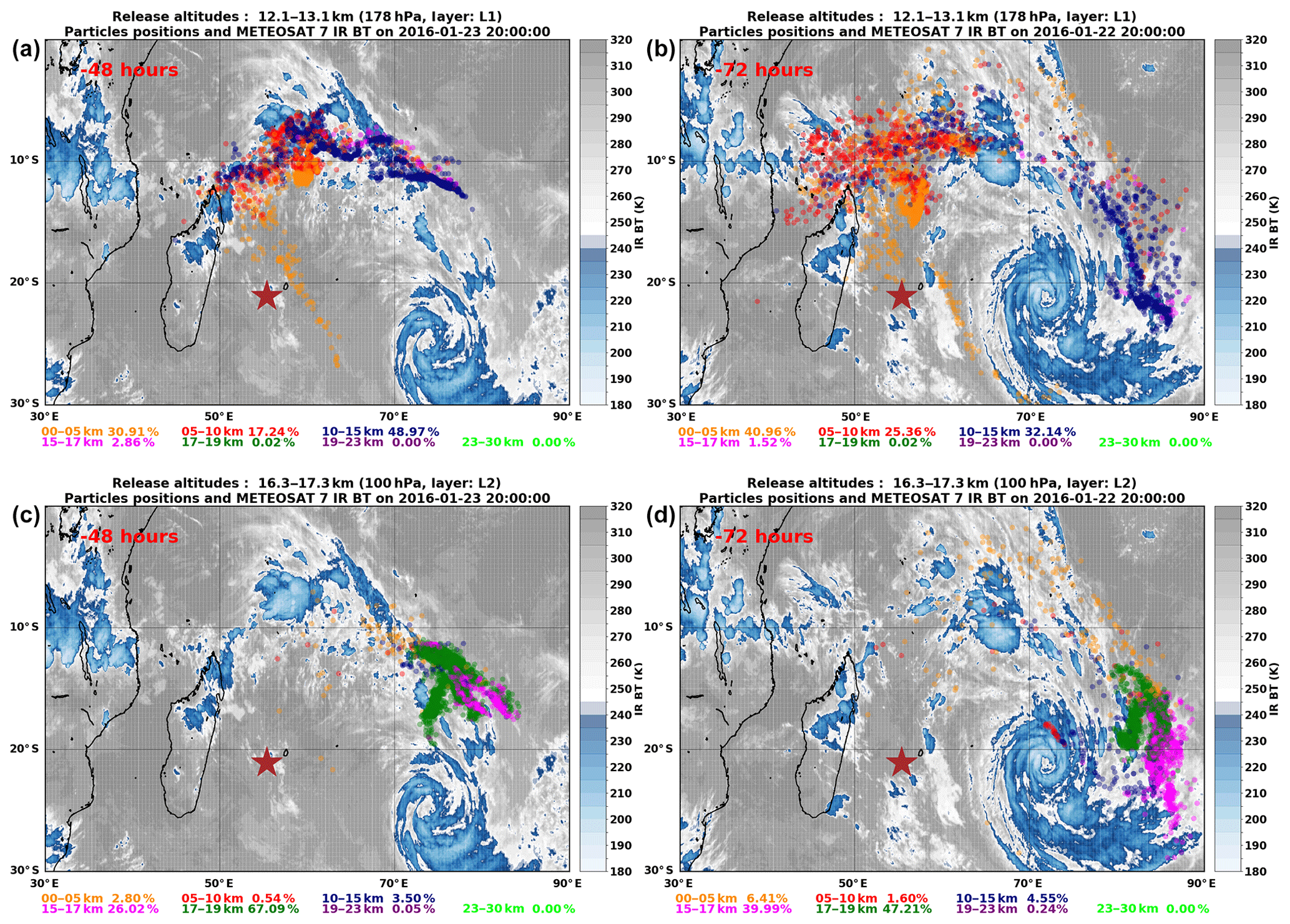
Figure 6Backward trajectories calculated with the FLEXPART model for the CFH flight on 25 January 2016. In (a) and (b), backward trajectories were initialized at 178 hPa (layer L1) on 25 January 2016. The particle positions 2 d before (on 23 January 2016 at 20:00 UTC; a) and 3 d before (on 22 January 2016 at 20:00 UTC; b) are shown with respect to the Meteosat-7 cloud distribution at those times. The altitude range of the particles (e.g., 0–5 km) and the percent of particles in that altitude range are indicated according to a color code shown in the bottom of each panel. (c, d) Same as (a) and (b) but for backward trajectories initialized at 100 hPa (layer L2) on 25 January 2016.

The ability of FLEXPART to represent isolated deep convective cells is limited due to the 0.15^∘ × 0.15^∘ spatial resolution of the ECMWF operational fields. At that resolution, isolated deep convective cells are not fully resolved in the ECMWF vertical wind field, and their updraft intensity and the altitude of the level of neutral buoyancy could be underestimated. However, the vertical transport of convective cells organized at mesoscale such as convection in tropical cyclones that cover several degrees in latitude and longitude is better resolved by the 0.15^∘ × 0.15^∘ ECMWF meteorological fields. Recent improvements of the ECMWF IFS model have enhanced its forecasting skills of tropical cyclones (Magnusson et al., 2019). Hence, the FLEXPART back trajectories driven by the ECMWF operational wind field give a qualitative sense of convective origins of vertical layers measured at Maïdo in relation to tropical cyclones.

According to FLEXPART, layer L1 measured above the Maïdo Observatory on 25 January 2016 ∼ 18:30 UTC has two different origins. At 2 d before (Fig. 6a), 48 % of this air mass was below 10 km (with ∼31 % below 5 km) and ∼1000 km northeast of Réunion Island in a region with convective clouds with cold brightness temperatures less than 220 K (∼12 km). Therefore, we can infer that the majority of layer L1 was lifted by convection associated with TS Corentin 2 d prior to the launch. These trajectories are rather spread in the lower troposphere, suggesting that they experienced turbulent mixing and changes in wind direction in the lower troposphere. The rest of the trajectories are located higher in altitude, in the 10–15 and 15–17 km altitude ranges. They are also located above convective clouds but are less scattered than the trajectories in the lower troposphere, suggesting that these trajectories were less mixed with the surrounding upper troposphere.

At 3 d before (Fig. 6b), 66 % of layer L1 originated from the lower and middle troposphere (41 % within the 0–5 km layer, 25 % within the 5–10 km layer) over the northeastern convective region of TS Corentin and 32 % from the upper troposphere (within 10–15 km) above TS Corentin. The upper tropospheric branch had a counterclockwise rotation with an origin near TS Corentin, in agreement with the upper divergence associated with TS Corentin. Hence, most of the air mass was located either in the lower troposphere or near the top of convective clouds 3 d before.

Layer L2 measured at Maïdo on 25 January 2016 stayed in the upper troposphere and near the tropopause 2 d before reaching Réunion Island (Fig. 6c). The trajectories followed a counterclockwise rotation associated with Corentin's dynamics and were located ∼250 km north of the center of TS Corentin. Only 3 % of trajectories that originated in the lower troposphere were found. On 22 January at 17:00 UTC (3 d before the launch), the trajectories were located east of the center of Corentin (Fig. 6d). About 8 % of the trajectories were below 10 km (6.4 % below 5 km). Note that TS Corentin reached its peak intensity on 23 January 2016 at 06:00 UTC (pressure at the center of 975 hPa, 10 min maximum sustained winds of 110 km h⁻¹). Hence, according to FLEXPART back trajectories and the Meteosat-7 infrared images, the origin of layer L2 was traced back to the active convective regions of TS Corentin and its upper divergence dynamics, but a small fraction originated from the lower troposphere. However, due to the 0.15^∘ spatial resolution of the ECMWF winds used to drive FLEXPART, the vertical updrafts of the deepest convective clouds that may reach the tropopause region/lower stratosphere may not be well represented in FLEXPART.

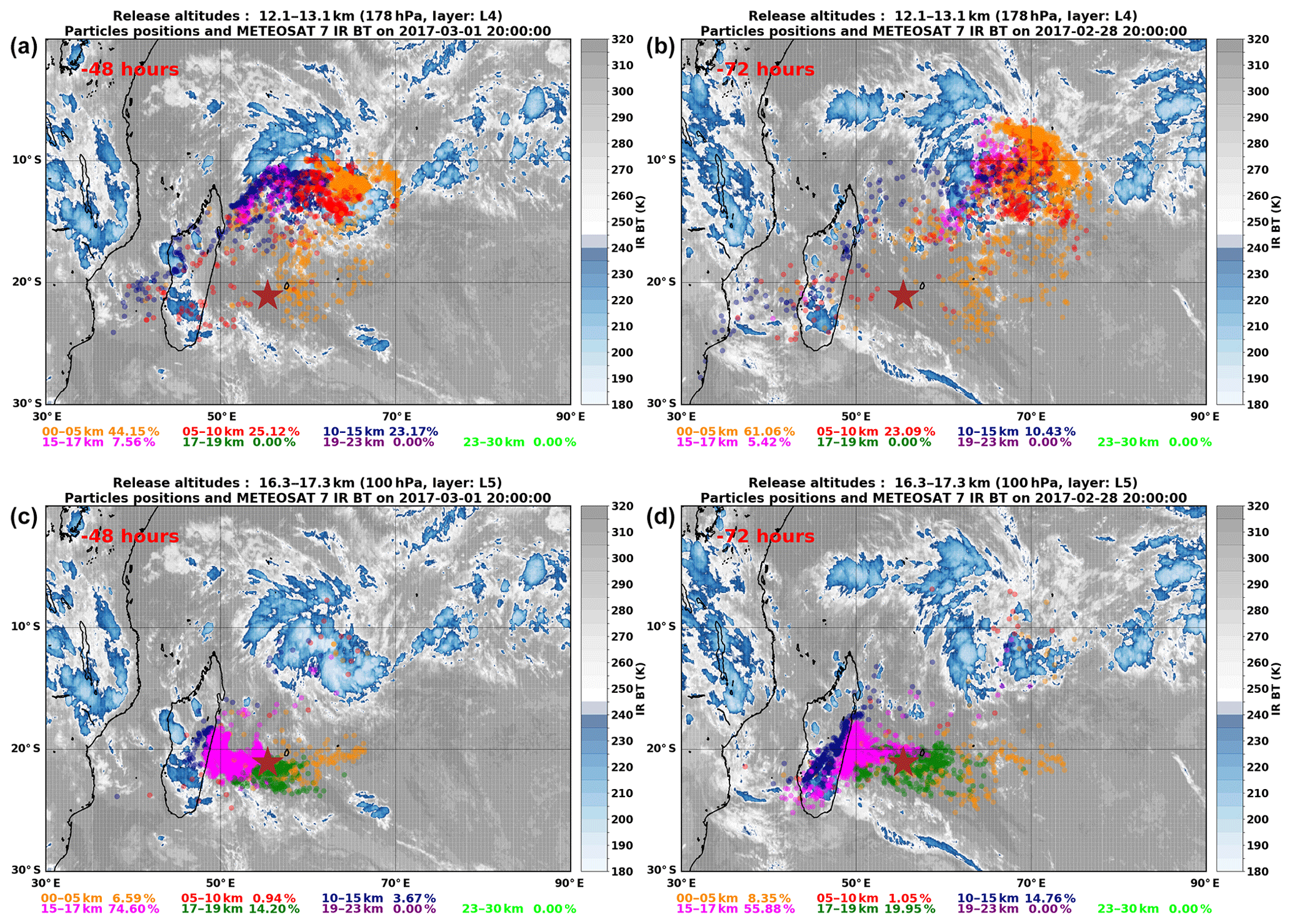
Figure 7Backward trajectories calculated with the FLEXPART model for the CFH flight on 3 March 2017. In (a) and (b), backward trajectories were initialized at 178 hPa (layer L4) on 3 March 2017. The particle positions 2 d before (on 1 March 2017 at 20:00 UTC; b) and 3 d before (on 28 February 2017 at 20:00 UTC; a) are shown with respect to the Meteosat-7 cloud distribution at those times. The altitude range of the particles (e.g., 0–5 km) and the percent of particles in that altitude range are indicated according to a color code shown in the bottom of each panel. (c, d) Same as (a) and (b) but for backward trajectories initialized at 100 hPa (layer L5) on 3 March 2017.

Figure 7 is similar to Fig. 6 but for back trajectories associated with the launch on 3 March 2017. Most of layer L4 measured on 3 March 2017 at 18:42 UTC was lifted by convection 800 km north of the island 2–3 d before (Fig. 7a and b). At 2 d before (Fig. 7a), the back trajectories indicate that a large fraction (69 %) of layer L4 is from the lower troposphere (below 10 km) over a convective region associated with TC Enawo. At 3 d before reaching Réunion Island (Fig. 7b), the trajectories were dispersed in the lower troposphere around the forming storm as Enawo was in the early stage of its formation at that time (tropical depression).

The FLEXPART back trajectories for layer L5 measured above the Maïdo Observatory on 3 March 2017 at 18:52 UTC stayed in the upper troposphere 2–3 d before the launch (Fig. 7c and d). The trajectories were confined to the same latitude band east and west of Réunion Island in a clear sky region away from convective clouds. It shows that air masses near the tropopause above Réunion Island on 3 March 2017 were most likely not affected by Enawo at this stage of its development as Enawo was still intensifying.

In a nutshell, the FLEXPART back trajectories clearly identify a convective origin for layers L1 and L4 sampled on 25 January 2016 and 3 March 2017 associated with TS Corentin and TC Enawo. The convective transport from the lower troposphere to the upper troposphere occurred roughly 2 d before each launch. As for the tropopause region over Réunion Island on 25 January 2016, FLEXPART back trajectories suggest that the air masses were embedded in TS Corentin's upper divergence dynamics over a region where convection was active. Deep convective clouds within TS Corentin may have reached the tropopause region (layer L2) on 23 January 2016 when the storm was at its peak intensity and may have influenced the water vapor content near the tropopause. On 3 March 2017, the tropopause region measured by the CFH sounding was not affected by deep convection associated with Enawo according to the model, at least not at the time of the observation. At that time, TC Enawo was still intensifying, and the deepest convective cloud developed later after 4 March 2017.

5.1 CFH and MLS comparisons

The CFH measurements analyzed in this study are compared to coincident MLS profiles. The match criteria used are ±18 h, ±500 km north–south distance (around ±5^∘ latitude) and ±1000 km east–west distance (around ±10^∘ longitude). The same match criteria are used in Davis et al. (2016). In addition, FLEXPART back trajectories initialized at each MLS pressure level are used to isolate the MLS profiles that were originating from TS Corentin and TC Enawo. Five and three matched MLS profiles are found for 25 January 2016 and 3 March 2017, respectively. On 25 January 2016, distances between the Maïdo Observatory and the matched MLS profiles ranged from 259 to 494 km with a mean distance of 346 km. The mean time difference for all matched profiles is 3.7 h. On 3 March 2017, the three matched MLS profiles are closer to the Maïdo Observatory with a mean distance of 281 km and are east of the island. However, a larger mean time difference of 16.4 h is observed for the matched MLS profiles.

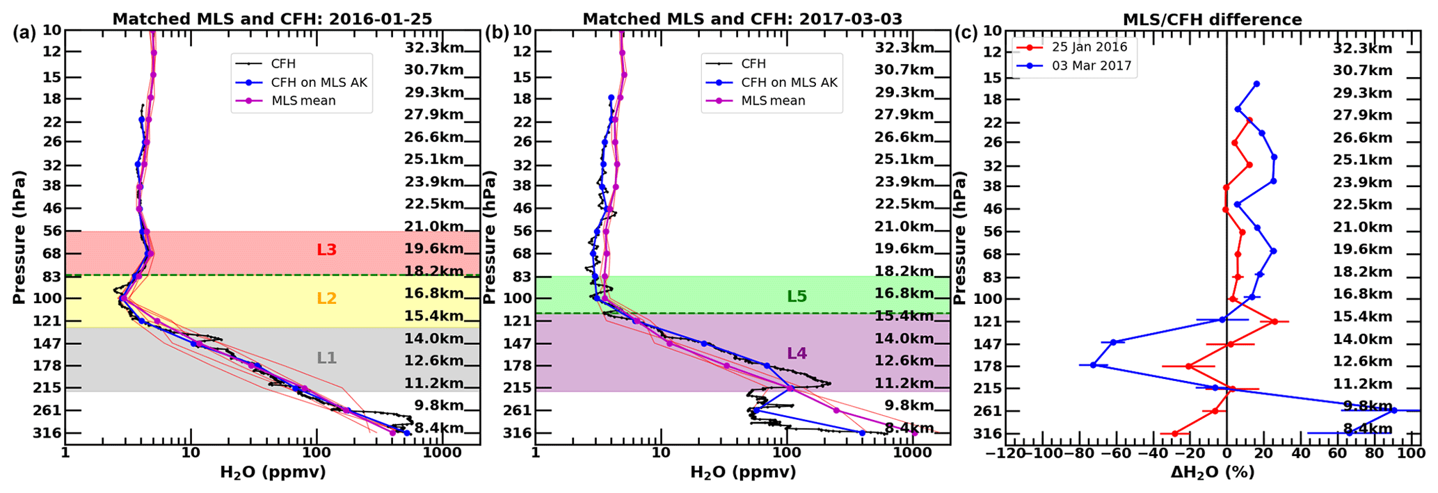
Figure 8(a, b) High-resolution (black line) and convolved (blue line) CFH water vapor profiles and closest-matched MLS profiles (thin red line) on 25 January 2016 (five profiles) and 3 March 2017 (three profiles). The mean MLS profile for each date corresponds to the thick magenta line. The location of the cold point tropopause is indicated by the dashed green line. Important water vapor features are shaded and named. (c) Mean percent difference between the convolved CFH water vapor profile and MLS coincident profiles on 25 January 2016 (red line) and 3 March 2017 (blue line). The horizontal bars indicate twice the standard error of the mean percent difference. Markers for each pressure level on 3 March 2017 are slightly offset in pressure for clarity. Corresponding altitude values for MLS pressure levels are also shown in each plot.

Download

To compare the high-resolution CFH water vapor profile to the MLS satellite data, we smooth the high-resolution sonde measurements to match the resolution of the satellite profiles using the MLS vertical averaging kernels, following the procedure described in Read et al. (2007) and Davis et al. (2016). The procedure for applying the MLS averaging kernels to a CFH profile requires an a priori profile as input; this is the same a priori profile used in the MLS retrieval. Figure 8 shows the matched MLS profiles and the CFH profiles convolved with the MLS averaging kernels. The matched MLS profiles on both dates illustrate how water vapor is more variable in the upper troposphere (between 316 and ∼147 hPa) compared to above it. The lower part of the tropopause layer from 147 hPa to the cold point tropopause (dashed green line in Fig. 8) is a transition region where water vapor mixing ratios become lower but could still be influenced by deep convective outflow. The application of the averaging kernel to the CFH profiles smoothes the fine-scale structures observed in the CFH profiles in Fig. 4 but still captures the deep layers of moist air in the upper troposphere between 261 and 147 hPa. To facilitate the comparison of CFH and MLS water vapor profiles in the upper troposphere and stratosphere where water vapor mixing ratios decrease by 3 orders of magnitude, we compute a mean percent difference of the MLS collocated profiles to the CFH and MLS data (i.e., percent difference = (MLS − CFH)∕((CFH + MLS)∕2) × 100). The same definition is used in Davis et al. (2016) and ensures that the distribution of percent difference at each pressure level is not skewed toward positive values larger than 100 % (since water vapor values are constrained to be positive). In addition, this facilitates the comparison with the study of Davis et al. (2016) that established a comparison between the 2004–2015 MLS water vapor data record and both routine monitoring and field campaign frost-point hygrometer balloon soundings at various stations around the world.

Several factors could explain why a dry bias exists between the mean MLS profile and CFH convolved profile on 3 March 2017. First, the 3 km deep wet layer observed in March 2017 in the CFH profile will not be well captured by MLS with a 2–3 km vertical resolution in the upper troposphere. In addition, the CFH launch on 3 March 2017 at 18:00 UTC was planned using FLEXPART Lagrangian trajectory analysis and satellite images in the days prior to the launch to sample the convective detrainment of TC Enawo. Therefore, the planning of the CFH launch on 3 March 2017 was optimal to sample moist air from convective detrainment, and an average of three MLS coincident profiles over a larger region/time window could be an underestimate of the storm-related moistening. It is also known that the stirring of air masses due to tropical cyclones generates a rather inhomogeneous atmospheric composition up to the TTL (Cairo et al., 2008, and references therein). It is possible that the CFH on 3 March 2017 sampled a fresher tropospheric filament with higher humidity than the three MLS profiles.

On 25 January 2016, the mean MLS water vapor profile agrees well with the convolved CFH profile over the entire lower tropical stratosphere within layer L3. The mean percent difference is $+\mathrm{7}\pm \mathrm{10}$ % (+0.3 ppmv) and lies within the previously published uncertainty of both instruments (Hurst et al., 2014; Vömel et al., 2007; Davis et al., 2016; Yan et al., 2016).

On 3 March 2017, larger differences of +18 % (∼ 0.6 ppmv) are observed in the lower stratosphere between 121 and 32 hPa. It is not clear why there are larger differences in the stratosphere on 3 March 2017. Both CFH instruments launched on 25 January 2016 and 3 March 2017 were prepared by the same operator and calibrated using the same recommended procedure. During these two flights, the CFH data streams were transmitted to receiving equipment on the ground through the InterMet radiosonde. From an instrumental standpoint, there is nothing that might explain a CFH dry bias on 3 March 2017 compared to 25 January 2016. Unfortunately, the CFH sondes are not recovered on the island after each flight as they land in the ocean, and thus it was not possible to examine in more details the instrument after the flight on 3 March 2017. To our knowledge, the CFH instrument on that night measured as well as it could in the stratosphere. Even though the CFH instrument launched on 3 March 2017 had a dry bias of 1 ppmv in the stratosphere, such a bias does not affect the results in this paper found for TC Enawo.

Overall, the MLS mean profile agrees within the uncertainty range with the CFH profile on 25 January 2016. On 3 March 2017, the MLS mean profile is drier than the CFH in the upper troposphere probably due to a lack of vertical resolution in MLS and inhomogeneity in the atmospheric composition.

5.2 Temperature anomaly

The hypothesis of a potential influence of convection on the CFH water vapor profile is further tested by analyzing the profile of the temperature anomaly. A seasonal mean (December–March) temperature profile is computed for the period 1997–2017 using the NDACC/SHADOZ dataset. The weekly NDACC/SHADOZ launch is performed at the airport in the north part of the island (Roland Garros, 20 m a.s.l.). The flying distance between the Maïdo Observatory and the airport is ∼20 km, so while boundary-layer temperature values will differ for the two sites, free troposphere and TTL temperature distributions can be compared as they are less influenced by topography. The seasonal mean CPT height is 17.31 km for the period December–March with a mean CPT temperature of 193.90 K (Table 1). The tropical tropopause is higher and colder during austral summer as a response to large-scale upwelling in the tropical stratosphere (Yulaeva et al., 1994) and convection (Highwood and Hoskins, 1998). The iMet radiosonde temperature profiles are then compared to the seasonal mean NDACC/SHADOZ temperature profile. The upper panels in Fig. 5 show temperature profiles from NDACC/SHADOZ and the iMet radiosonde. The black line shows the NDACC/SHADOZ seasonal mean temperature profile, while the red line corresponds to the iMet temperature profile observed at the Maïdo Observatory.

Table 1CPT properties (temperature and height) from the radiosonde launches on 25 January 2016 and 3 March 2017 and NDACC/SHADOZ seasonal mean (December–March) CPT properties (for the period 1997–2017).

Download Print Version | Download XLSX

A large positive temperature anomaly is observed on 25 January 2016 over a broad tropospheric region from 2 to 16 km (mean amplitude of +2.5 K) with a peak warming of +4.6 K at 10 km (magenta line in Fig. 5). On 3 March 2017, a warm temperature anomaly is mostly observed between 6 and 14 km (mean amplitude of +1.1 K) with a peak value of +3.1 K near 12 km. The stronger warming of the troposphere observed in January 2016 may be due to the strong 2015/2016 El Niño. The connection between interannual variations in tropical tropospheric temperature and ENSO is well established (e.g., Yulaeva and Wallace, 1994; Soden, 2000). Using 13 years of temperature data from the tropospheric channel of the microwave sounding unit (MSU-2), Yulaeva and Wallace (1994) showed that a tropospheric warming occurs almost uniformly over the tropics and that the magnitude of the warming is around 0.5–1 ^∘C for strong El Niño years. Chiang and Sobel (2002) updated the analysis of Yulaeva and Wallace to include the response to the strong 1997/1998 El Niño (ONI of +2.2 K in December–February 1998) and indicated an MSU-2 temperature anomaly of ∼1.2 K in January 1998 (cf. Fig. 1 of Chiang and Sobel, 2002). Note that the MSU-2 temperature data used in these studies provide a measure of the mean temperature of the 1000–200 mb layer (corresponding to the surface to ∼11 km using a scale height of 7 km). Thus, part of the strong tropospheric warming (especially in the lower part of the troposphere) observed in January 2016 may be due to the strong 2015/2016 El Niño (ONI of +2.5 K in December–February 2016). Assuming a tropospheric warming of ∼1 K in response to a strong El Niño, the magnitude of the upper tropospheric warming observed on 25 January 2016 (mean amplitude of 3.4 K between 10 and 14 km) becomes more similar to the one observed on 3 March 2017 (mean amplitude of 1.9 K between 10 and 14 km) if the effect of the 2015/2016 El Niño is removed.

Figure 5 indicates cold temperature anomalies within 16–19 km above the tropospheric warm anomalies on 25 January 2016. The mean amplitude of the 16–19 km temperature anomaly is −1.6 K with a maximum cooling of −3.6 K at 18 km. A similar feature is observed on 3 March 2017 with a cooling between 14 and 17 km, a mean amplitude of −2 K, and maximum cooling of −4.5 K at 15.1 km. The upper tropospheric warming and near tropopause cooling observed on both dates is consistent with a temperature response to deep convection (e.g., Sherwood et al., 2003; Holloway and Neelin, 2007; Paulik and Birner, 2012). The cooling around the tropopause can be explained by either radiative cooling by cirrus clouds over the regions of deep convection (Hartmann et al., 2001) or diabatic cooling through convective detrainment (Sherwood et al., 2003; Kuang and Bretherton, 2004). CPT properties can also be modified by convectively driven waves (Zhou and Holton, 2002; Randel et al., 2003).

Paulik and Birner (2012) investigated the deep convective temperature signal based on SHADOZ ozone and temperature data. Low ozone concentrations in the upper troposphere are indicative of convective transport from the boundary layer. They looked at temperature anomalies corresponding to low ozone anomalies between 12 and 18 km, thus temperature anomalies influenced by deep convection. A strong warming was observed near the level of main convective outflow at ∼12 km, and cooling was more pronounced above ∼15 km and near the CPT at ∼17 km. Thus, the upper tropospheric warm temperature anomalies, as well as cold temperature above 15 km and near the tropopause in Fig. 5, are consistent with a deep convective temperature signal. Paulik and Birner's study also showed that the amplitude of the temperature anomalies increases as convection strengthens with a warming of ∼2 K in the upper troposphere and a cooling of around −3 K near 16 km (cf. Fig. 5 of Paulik and Birner, 2012). Using CloudSat observations of deep convective clouds and constellation Observing System for Meteorology, Ionosphere and Climate (COSMIC) GPS temperature profiles, they showed that the deep convective temperature signal (i.e., anomalously warm upper troposphere and an anomalously cold upper TTL) was only present for deep convective clouds above 15 km. Although the magnitude of the temperature anomalies decreases with increasing distance from convection, they observed a deep convective temperature signal during December–February ∼3500 km away from the convective event. Within 1000 km of the deepest convection (deep convective clouds above 17 km), the convective temperature anomaly exceeds 0.75 K in the upper troposphere and ranges from −1 to −2.0 K near 16 km. In our case, the deepest convective clouds with cloud tops colder than 190 K were 1000 km away from the island on 22–25 January 2016 and were closer to the island at ∼500 km on 28 February–3 March 2017 (Fig. 2). Although deep convective clouds observed on 22–25 January 2016 and 28 February–3 March 2017 were not in the immediate vicinity, relatively fast-moving gravity waves caused by deep convection could spread the deep convective temperature signals over large regions in short amounts of time (Holloway and Neelin, 2007). The temperature anomalies in Fig. 5 are much larger than those reported by Paulik and Birner for temperature profiles around the time (±6 h) and location of deep convection (within 1000 km). However, we are studying deep convective temperature anomalies associated with two individual events, while their deep convective temperature signal was estimated using 4 years of COSMIC data. Therefore, their estimates correspond to an average deep convective temperature signal; such a signal is likely larger when considering larger/more organized convective events such as tropical storms.

Hence, the temperature anomalies derived from the 25 January 2016 and 3 March 2017 profiles are consistent with a deep convective outflow in the upper troposphere.

5.3 Water vapor anomaly

To further assess the impact of TS Corentin and TC Enawo on the upper troposphere–lower stratosphere (UTLS) water vapor content, we compare the convolved CFH profiles to a monthly climatological MLS water vapor profile as there are no long-term stratospheric water vapor measurements on Réunion Island. For each year between 2004 and 2017, MLS water vapor profiles within ±5^∘ latitude and ±10^∘ longitude of Réunion Island and over a period of 15 d surrounding the launch date, i.e., 10 January–9 February for 25 January 2016 and 16 February–18 March for 3 March 2017, are used to define a monthly climatological water vapor profile. We also computed a non-convective monthly climatological MLS water vapor profile by excluding MLS water vapor profiles with coincident low upper-tropospheric ozone (probably affected by convection; Paulik and Birner, 2012). The non-convective and monthly climatological MLS water vapor profile (using all profiles) looks very similar (not shown). Thus, the climatological MLS water profile using all profiles is used for comparison with the water vapor measurements on 25 January 2016 and 3 March 2017.

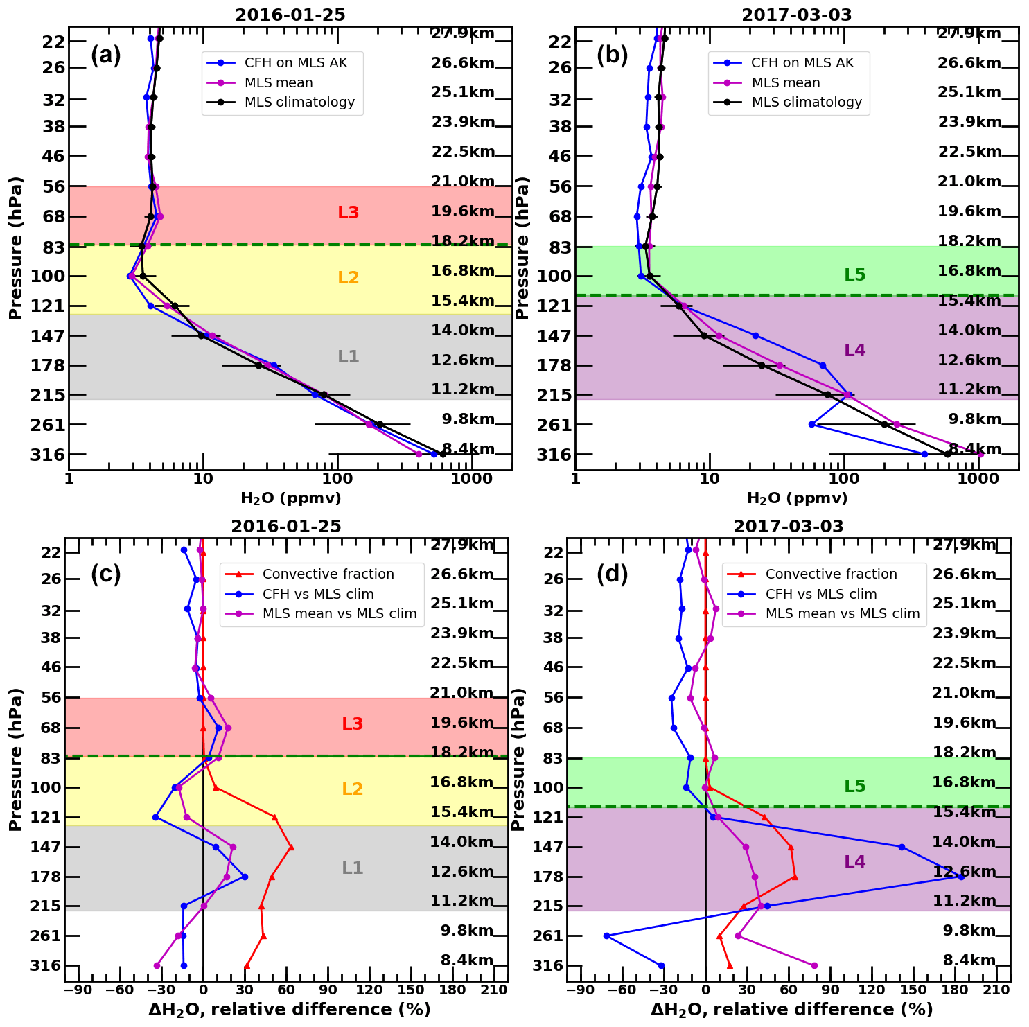
Figure 9(a, b) Convolved CFH water vapor profiles (blue line), mean of closest-matched MLS profiles (magenta) and monthly mean climatological MLS water vapor profile for Réunion Island (black line; see text for definition of the MLS climatological profile) on 25 January 2016 (a) and 3 March 2017 (b). The horizontal bars in black correspond to the ± 1 standard deviation range. (c, d) Relative difference between the convolved CFH water vapor profile and the MLS climatological profile for Réunion Island (blue line) and the mean of closest-matched MLS profiles and the MLS climatological profile (magenta line). The convective fraction computed with FLEXPART back trajectories and Meteosat-7 infrared brightness temperature is shown in red. Corresponding altitude values for MLS pressure levels are also shown in each plot.

Download

The monthly climatological MLS water vapor profiles and CFH convolved profiles are shown in Fig. 9. Both monthly climatological water vapor profiles have comparable minimum water vapor mixing ratios at 83 hPa (3.5±0.6 ppmv and 3.3±0.5 ppmv for the January and March climatologies, respectively). In the upper troposphere (316–178 hPa), the climatologies have mean values of 277.6±269.2 ppmv and 266.1±253.2 ppmv for January and March, respectively. High variability in the UT is consistent, with deep convection being more active during austral summer. Higher UT water vapor content in January relative to March is in agreement with the fact that the austral summer season reaches its peak in January/February. Both January and March climatologies have comparable TTL (147–68 hPa) water vapor content (5.3±1.8 ppmv and 5.1±1.7 ppmv for January and March, respectively). The climatological mean stratospheric (56–22 hPa) value is 4.2±1.3 ppmv for both months.

Relative water vapor differences are defined with respect to the monthly climatological profile (i.e., relative difference = (CFH − MLS climatology)∕MLS climatology × 100) and are displayed in Fig. 9c and d. In addition to the CFH convolved profile, we also compared the mean of MLS coincident profiles to the MLS monthly climatological profile for 25 January 2016 and 3 March 2017.

On 25 January 2016, the mean of MLS coincident profiles and the CFH convolved profile shows a peak of ∼30 % or 7.7 ppmv in the relative difference with the MLS climatology in layer L1, but the pressure level of this peak differs in the two profiles with a peak at 178 hPa for the CFH convolved profile and 147 hPa for the mean of coincident MLS profiles.

To further evaluate the portion of the profiles that were influenced by convection, we calculated a convective fraction profile. For each pressure level depicted in Fig. 9, 50 000 FLEXPART back trajectories were initialized. A back trajectory was tagged as convectively influenced when the IR brightness temperature observed by Meteosat-7 falls below 230 K over the previous 7 d and if the altitude of the back trajectory falls below 5 km, indicating a lower tropospheric origin. Hence, the convective fraction profile represents the percentage of trajectories for each pressure level that was considered convective following those criteria. The convective fraction profile reaches a maximum of 60 % at 147 hPa and confirms that layer L1 and the bottom part of layer L2 are convective. The FLEXPART back trajectories from Fig. 6 and the values of the convective fraction profile confirm that the positive water vapor anomalies observed in layer L1 are associated with the convective outflow of TS Corentin.

On 3 March 2017, the hydration of the upper troposphere in layer L4 (between 215 and 121 hPa) is much more pronounced in the CFH convolved profile with a peak value of ∼180 % or 45 ppmv at 178 hPa. For the mean of MLS coincident profiles, the moistening is not as large with a relative difference of 36 % or 8.7 ppmv at 178 hPa. The convective fraction profile had values of 60 % at 178 and 147 hPa, confirming that layer L4 was influenced by convection.

Ray and Rosenlof (2007) used measurements from AIRS to assess the impact of tropical cyclones in the Atlantic and Pacific basins on the amount of water vapor in the tropical UT. They showed that tropical cyclones can hydrate a deep layer of the surrounding upper troposphere by ∼ 30–50 ppmv or more within 500 km of the eye compared to the surrounding average water vapor mixing ratios (cf. Fig. 3 of Ray and Rosenlof, 2007). They also looked at the evolution of UT water vapor changes as a function of the storm intensity as measured by the peak wind speed (cf. Fig. 5 of Ray and Rosenlof, 2007). In both the Atlantic and western Pacific basins, the average water vapor at 223 hPa around the storm center steadily increased from 4 to 5 d prior to peak cyclone intensity to 2 d following peak cyclone intensity. The average water vapor enhancement in the two ocean basins was from 5 to 20 ppmv with an increase as high as 30–40 ppmv for some cyclones in the western Pacific. The CFH launch on 3 March 2017 at 18:00 UTC occurred 3.5 d before Enawo reached its peak intensity on 7 March at 06:00 UTC (pressure at the center of 932 hPa, 10 min maximum sustained winds of 204 km h⁻¹), and the storm center was ∼700 km away from the island. Thus, deep convection associated with TC Enawo may have caused the strong increase in UT water vapor observed on 3 March 2017. Ongoing work with MLS data to apply the methodology of Ray and Rosenlof (2007) to assess hydration of the UTLS by tropical cyclones for the 2004–2017 cyclone seasons in the southwest Indian Ocean is under way. This will be the focus of a future study, but preliminary results indicate water vapor differences of 35 % to 48 % at between 178 and 261 hPa for category 2 to 4 hurricanes on the Saffir–Simpson scale. Ray and Rosenlof (2007) indicated that tropical cyclones hydrate a deep layer of the UT in the vicinity of the cyclones by up to 50 % above monthly mean water vapor mixing ratios. Therefore, our estimate of UT water vapor increases of 20 % to 100 % using CFH and MLS data for TS Corentin (category 1 hurricane at its peak intensity) and TC Enawo (category 4 hurricane at its peak intensity) are in broad agreement with our estimates based on the 2004–2017 MLS data and the study of Ray and Rosenlof (2007).

At 100 hPa (within layer L2), both MLS and CFH data are 20 % (−0.7 ppmv) below the climatological monthly mean values on 25 January 2016. This would be consistent with the near tropopause cooling observed in Fig. 5 and the presence of deep convection around Réunion Island. In addition, TTL cirrus clouds were observed north of the island on both dates (Fig. 5). Convectively generated or in situ cirrus clouds in the TTL can dehydrate the tropopause region. Jensen et al. (1996) showed that ice clouds formed by large-scale vertical motions can result in the depletion of the water vapor mixing ratio by about 0.4 ppmv. Chae et al. (2011) investigated temperature and water vapor changes due to clouds in the TTL using MLS, CALIPSO and CloudSat datasets. They noted that generally clouds humidify the environment near 16 km (∼100 hPa) or lower but dehydrate the TTL above 16 km.

On 25 January 2016, CFH and MLS data are 11 % (+0.4 ppmv) and 18 % (+0.7 ppmv) moister than the climatological values at 68 hPa (within layer L3) above the tropopause. Observational and modeling studies have indicated that overshooting convection can moisten the lower stratosphere by injecting water vapor or ice crystals directly above the overshooting clouds (e.g., Danielsen, 1993; Corti et al., 2008; Dauhut et al., 2015; Frey et al., 2015; Allison et al., 2018). In our case, the observation on 25 January 2016 was not made close to the deepest convective clouds that were ∼1000 km north of the island (Fig. 2) but was downwind of TS Corentin, as shown by the FLEXPART analysis (Fig. 6). However, FLEXPART back trajectories indicate that the air masses at 68 hPa (layer L3) originate from the southeast Indian Ocean in the 20–30^∘ S latitude band, where the MLS water vapor anomaly for January 2016 is around 0.5 ppmv most likely due to the impact of the 2016 strong El Niño event. Hence, the positive anomaly against the climatological value can also be explained by horizontal advection from the southeast Indian Ocean toward Réunion Island.

It is difficult to conclude whether TC Enawo had a direct impact on water vapor in the lower stratosphere by using only the CFH observation on 3 March 2017. The FLEXPART analysis indicated that the CFH sounding did not sample the lower stratosphere downwind of Enawo.

Ongoing work with the mesoscale model Meso-NH at a 2 km resolution for TC Enawo for the period 2–7 March 2017 indicates that deep convective clouds within 500 km of the cyclone's eye can inject ice crystals and moisten the lower stratosphere, resulting in an average anomaly of ∼2 ppmv within 500 km of the tropical cyclone's eye. The strongest humidification in the lower stratosphere (17–19 km, ∼ 88–66 hPa) was found after 4 March when the storm stalled over the ocean (while intensifying) and after 6 March when it reached its peak intensity. Thus, the CFH observation on 3 March 2017 was made before TC Enawo had influenced the lower stratosphere above 100 hPa. This is further confirmed by the fact CALIOP did not have a lower stratospheric signal in Fig. 6.

Tropical cyclones are unique among tropical convective systems in that they persist for many days and thus could affect the UTLS more than other mesoscale convective systems. Clouds in tropical cyclones often reach to and sometimes beyond the tropopause (e.g., Romps and Kuang, 2009). Allison et al. (2018) have investigated the vertical transport of water vapor by the 2013 tropical cyclone Ingrid in the North Atlantic. Results of their high-resolution numerical simulations indicated that hydration occurred between 17.5 and 21 km (83 to 56 hPa) due to the injection of ice crystals. As the exact role of deep convection, and tropical cyclones in particular, in hydrating the lower stratosphere is still under debate, additional TTL observations of water vapor and modeling work are needed to quantify the overall impact of convection on TTL and MLS water vapor. High-resolution (2 km) numerical simulations of TC Enawo for the period 2–7 March 2017 are underway to gain a closer look at the effect of TC convection on TTL temperature and water vapor. This work will be the subject of a subsequent study.