2.1 GEM-MACH

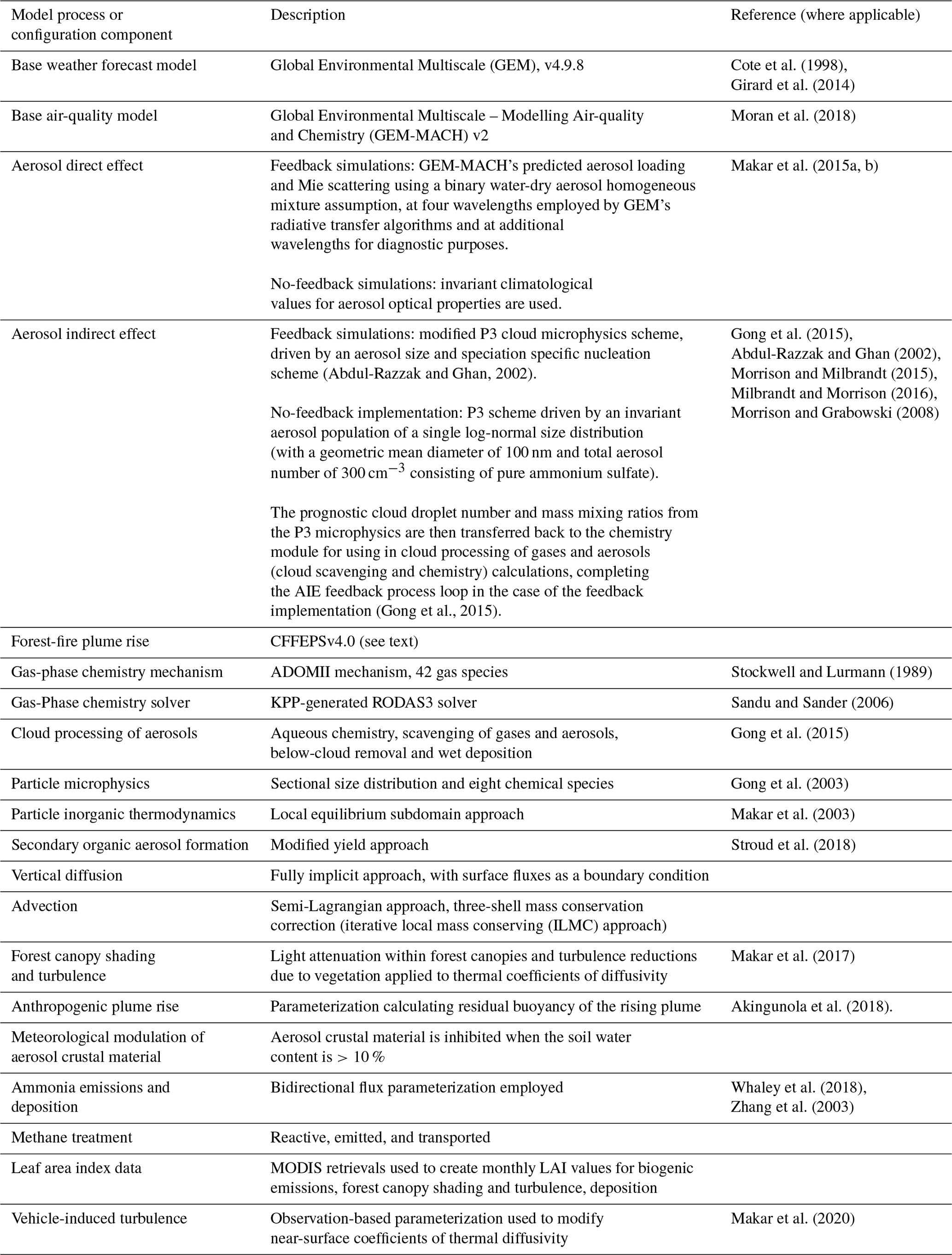
The Global Environmental Multiscale – Modelling Air-quality and CHemistry (GEM-MACH) model in its online coupled configuration has been described elsewhere (Makar et al., 2015a, b; Gong et al., 2015, 2016). The model combines the Environment and Climate Change Canada Global Environmental Multiscale weather numerical weather prediction model (GEM; Cote et al., 1998; Girard et al., 2014) with gas and particle process representation using the online paradigm, with options for climatological versus full coupling between meteorology and chemistry. GEM-MACH's main processes for the two configurations employed here are described in Table 1.

Table 1GEM-MACH model configuration details and references.

Download Print Version | Download XLSX

Simulations were carried out with a 2.5 km horizontal grid cell spacing over a 900×1370 grid cell domain, covering most of western Canada and the USA (Fig. 1). The meteorological boundary conditions for the simulation were a combination of 10 km resolution GEM forecasts updated hourly (themselves originating in data assimilation analyses of real-time weather information; Fig. 1a) and 2.5 km GEM simulations (Fig. 1c) employing, in the northern portion of this 2.5 km domain, the Canadian Land Data Assimilation System (Carrera et al., 2015), to better simulate surface conditions. Both “feedback” and “no-feedback” simulations were carried out on a 30 h forecast cycle (Fig. 2). Following the usual practice for weather forecasts, the analysis-driven meteorological forecasts at 10 km resolution were updated operationally every 24 h at 12:00 UT (Fig. 2a). These 10 km resolution weather forecasts were used to drive a 30 h, 10 km resolution GEM-MACH forecast (Figs. 1b and 2b), which employed ECMWF reanalysis data for North American chemical lateral conditions (Innes et al., 2019). The 10 km resolution weather forecasts were also used to drive a 30 h meteorology-only forecast at 2.5 km resolution on the high-resolution domain (Figs. 1c and 2c). The last 24 h of the 10 km resolution GEM-MACH forecast was also used to provide chemical lateral boundary conditions for the 24 h 2.5 km online coupled GEM-MACH simulation (Figs. 1c and 2d). The last 24 h of the 2.5 km GEM simulation was used as meteorological initial and boundary conditions for the 24 h 2.5 km online coupled GEM-MACH simulation (Figs. 1c and 2d). The two stages of meteorology-only simulations were carried out to prevent chaotic drift from the observed meteorology and to allow spin-up time for the cloud fields of that meteorology to reach equilibrium (6 h timeframe). Chemical initial concentrations for each consecutive forecast within the 2.5 km GEM-MACH model domain were “rolled over” or “daisy-chained” between subsequent forecasts without chemical data assimilation. Forecast performance scores presented here are for the inner 2.5 km domain from this set of linked 24 forecast simulations, mimicking operational forecast conditions.

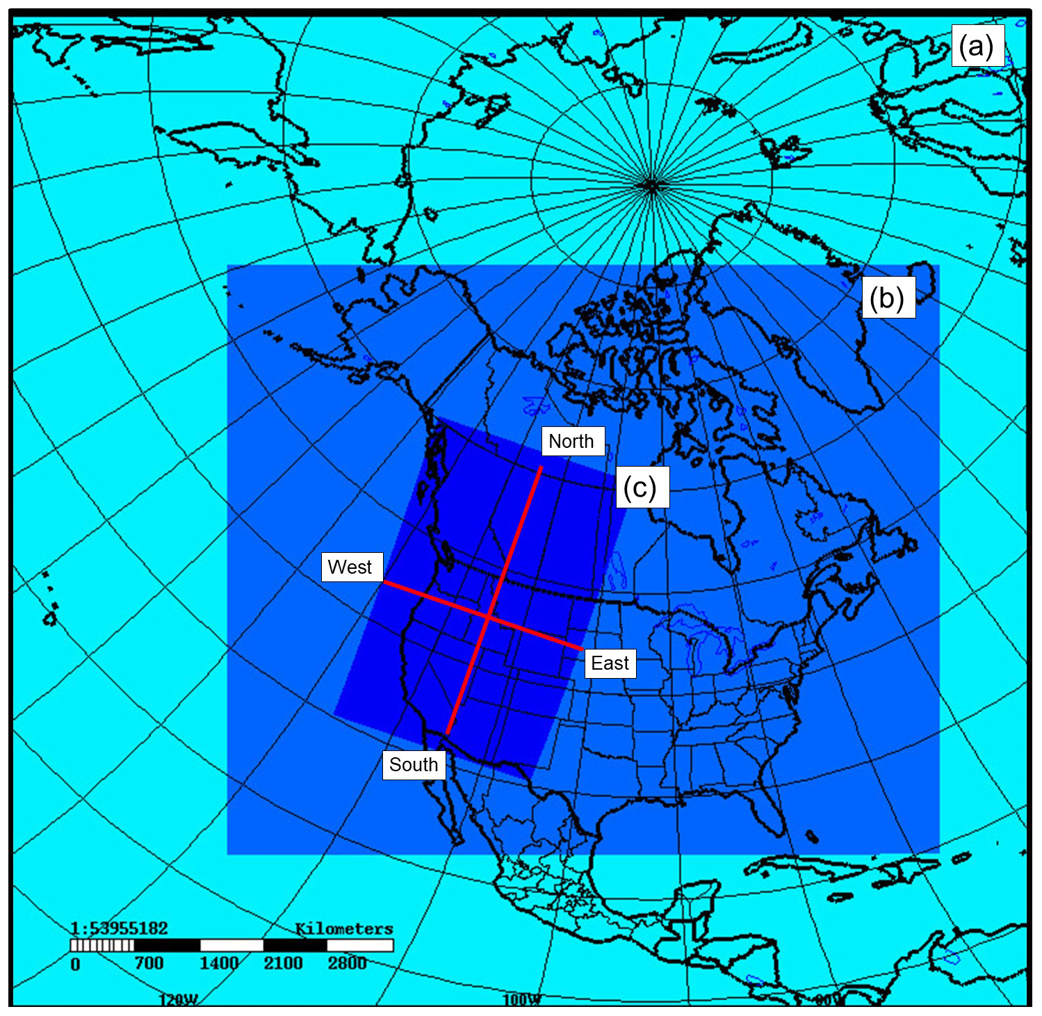
Figure 1GEM-MACH domains: (a) GEM meteorology 10 km resolution forecast domain. (b) GEM-MACH 10 km resolution forecast domain. (c) GEM-MACH inner 2.5 km grid resolution forecast domain for comparison to observations. Red lines indicate locations of illustrative south–north and west–east cross sections appearing in subsequent analysis in the text.

Figure 2Example time sequencing of model simulations used to generate the 2.5 km GEM-MACH simulations carried out here. Green lines and print indicate GEM (weather forecast only) simulations), and blue lines and print indicate 2.5 km GEM-MACH simulations. Arrows indicate data flow (light green: meteorological information; light blue: chemical information). Steps (a) through (h) illustrate the sequence of forecasts used to generate 2 consecutive days of 2.5 km GEM-MACH simulations. Note that online coupling occurs only at the 2.5 km GEM-MACH forecast level, in this sequencing.

Download

2.2 CFFEPS version 4.0: online forest-fire plume-rise calculations

In addition to the above algorithm improvements relative to GEM-MACH implementations, this model system setup has incorporated the first online calculation of forest-fire plume rise by energy balance driven using online meteorology, in a new version of the Canadian Forest Fire Emissions Prediction System (CFFEPS). The algorithms of CFFEPSv2.03 are described in detail and evaluated elsewhere (Chen et al., 2019) but will be outlined briefly here, as well as subsequent modifications to this forest-fire emissions processing module.

CFFEPS combines near-real-time satellite detection of forest-fire hotspots with national statistics of burn areas by Canadian province and by specific fuel type across North America. CFFEPS assumes persistence fire growth in the subsequent 24 to 72 h forecasts with hourly fuel consumed calculated (kg m⁻²), based on GEM forecast meteorology and predicted fire intensity and fuel consumption in grid cells representing fire locations. The modelled fire fuel consumption is then linked with combustion-phase specific emission factors (g kg⁻¹) for fire specific emissions and chemical speciation. Fire energy associated with the modelled combustion process is also estimated and is used in conjunction with a priori forecasts of meteorology within the column to determine plume rise. In its offline/non-coupled configuration (Chen et al., 2019), CFFEPS carries out residual buoyancy calculations at five preset pressure levels (surface, 850, 700, 500, 250 mb). CFFEPS predicts plume injection heights, which are in turn used to redistribute the mass emissions below the plume top to the model hybrid levels. This approach employed in CFFEPSv2.03 provided a substantial improvement in forecast accuracy relative to the previous approach employing modified Briggs (Briggs, 1965, 1984; Pavlovic et al., 2016) plume-rise formulae in the offline GEM-MACH forecast system (Chen et al., 2019). A recent evaluation of the plume heights predicted by CFFEPS was carried out utilizing MISR and TROPOMI satellite retrieval data (Griffin et al., 2020). A total of 70 cases studied using MISR data showed good agreement between satellite and CFFEPS-predicted maximum and mean plume heights (maximum plume height observed versus predicted values and standard deviations: 1.7±0.9 versus 2.0±1.0 km; mean plume height observed versus predicted: 1.3±0.6 versus 1.3±0.4 km). A larger number of case studies using TROPOMI data (671 in total) also showed a reasonable agreement, with CFFEPS showing a small tendency to overpredict heights (maximum observed versus predicted plume heights 2.2±1.6 versus 2.5±1.2 km; mean observed versus predicted plume heights 0.7±0.5 versus 1.1±0.6 km).

However, other work has shown the substantial impact of large forest fires on regional weather (Makar et al., 2015a; Palacios-Peña et al., 2018; Baró et al., 2017), including changes to the surface radiative balance and atmospheric stability. These findings imply that plume-rise calculations employing an a priori weather forecast lacking the impact of fire plumes via the ADE and AIE may not accurately predict the weather conditions critical to subsequent forest-fire plume-rise prediction. In order to study this possibility, and to allow forest-fire plumes to influence weather and hence subsequent fire spread/growth, several changes were made to the CFFEPS implementation, resulting in version 4.0 of CFFEPS, used here. The process flow within CFFEPSv2.03 versus CFFEPSv4.0 is compared in Fig. 3. The original C language CFFEPSv2.03 code was converted to FORTRAN90 and, following successful offline comparisons to the original code, was then integrated as an online subroutine package within GEM-MACH itself, with the near-real-time satellite hotspot data and location fuel parameters being read into GEM-MACH directly (CFFEPSv4.0 is this new online package). A key advantage of the CFFEPSv4.0 subroutine integration within GEM-MACH is that the residual buoyancy calculations for plume injection heights are now carried out over the model hybrid model layers, rather than the five coarse-resolution, prescribed pressure levels of CFFEPSv2.03, making complete use of GEM-MACH's detailed vertical structure. Additionally, CFFEPSv4.0 allows plume-rise calculations to be updated during model runtime. When GEM-MACH is run in online coupled mode, the ADE and AIE implementations allow model-generated aerosols to modify the predicted meteorology, in turn influencing predicted fire emissions and plume rise, closing these feedback loops. The online implementation of CFFEPSv4.0 thus allows us to investigate the effects of meteorology on subsequent forest-fire plume development, the changes to modelled aerosol compositions, and, ultimately, the feedbacks to weather.

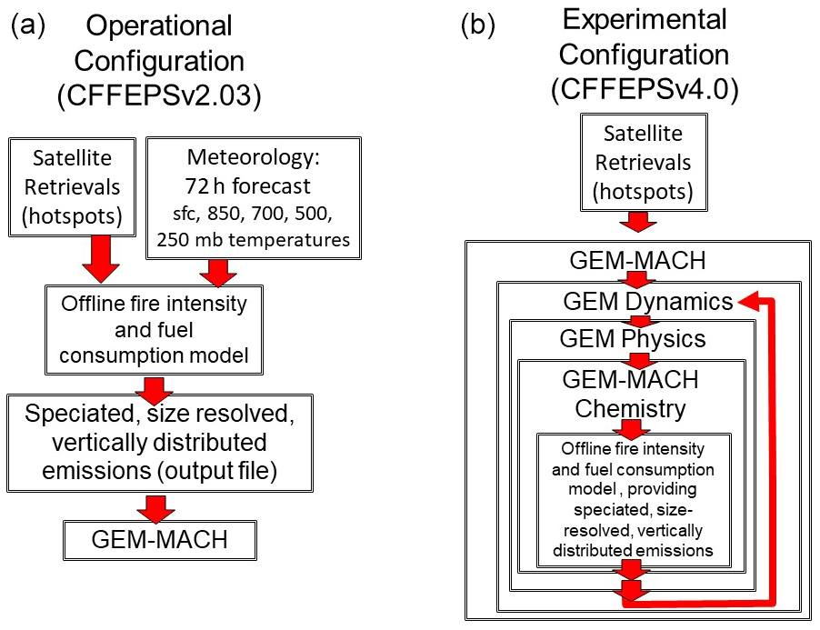
Figure 3Process comparison between original (CFFEPSv2.03, a) and online (CFFEPSv4.0, b) forest-fire emissions and vertical plume distribution algorithms.

Download

The formation of particles from forest fires affects meteorology on the larger scale via the ADE and AIE, in turn modifying the regional-scale atmospheric features affecting fire growth, such as the temperature profiles below forest-fire plumes. However, we note that CFFEPSv4.0 employs forest fire heat to determine plume rise as a subgrid-scale thermodynamic process parameterization rather than a very high-resolution explicit fire growth parameterization; the very local-scale weather modifications due to the addition of forest-fire heat to the atmosphere are not incorporated into fire spread or GEM microphysics. Specifically, when the feedback version of GEM-MACH incorporating CFFEPSv4.0 is used in its online coupled configuration, CFFEPSv4.0 uses estimates of the heat released to calculate forest-fire plume rise. These calculations employ lapse rates at the fire locations, that with feedbacks enabled, include the ADE and AIE generated by forest-fire aerosols on atmospheric stability within the current online coupled model time step. This is in contrast to earlier offline implementations of CFFEPS, which made use of a priori non-feedback weather forecast lapse rates. To the best of our knowledge, this is the first implementation of a dynamic forest-fire plume injection height scheme incorporated into an online coupled high-resolution, operational air-quality forecast modelling system. The impact of this feedback on both weather and air-quality can be substantial, as we show in the following sections.

The locations of the daily forest hotspots detected during the study period and the corresponding magnitude of the daily PM_2.5 emissions generated by CFFEPS for each hotspot are shown in Fig. 4. Individual hotspots with the highest magnitude emissions are located in the state of Nevada (Fig. 4a, southern boxed region). However, the largest ensemble emissions from a suite of hotspots occur in northern Alberta (Fig. 4a, northern boxed region). Expanded views of the northern Alberta and Nevada hotspots are shown in Fig. 4b and c respectively – the use of smaller symbols shows that the Alberta hotspots are groups representing large spreading fires, which are overplotted in Fig. 4a, while the Nevada hotspots indicate single fires of small spatial extent and duration rather than larger spreading fires. The Alberta fires are thus the most significant sources of forest-fire emissions in the study domain for the period analyzed here.

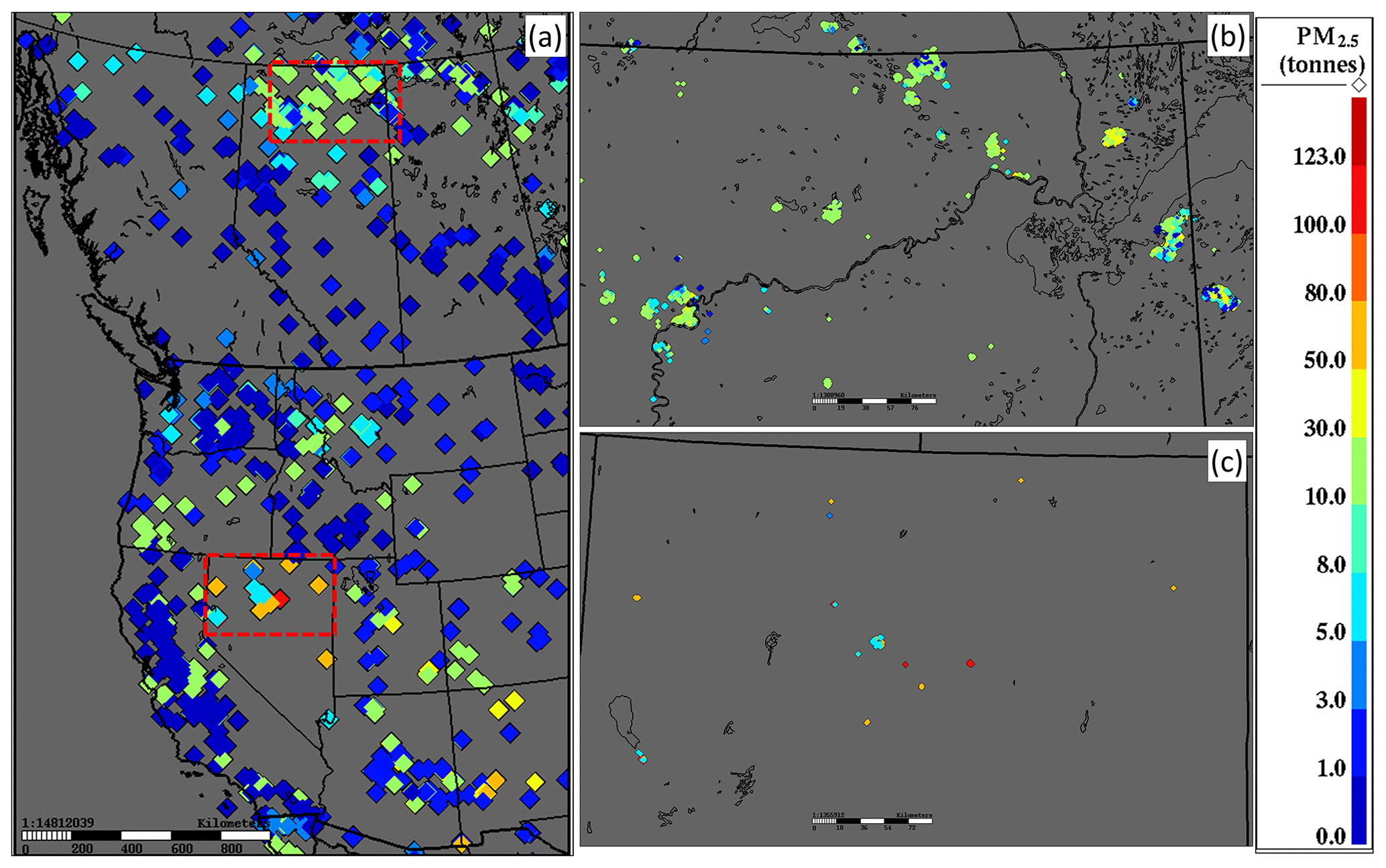
Figure 4Hotspot locations during the study period, colour-coded by daily total tonnes PM_2.5 emitted. (a) Entire model 2.5 km domain, with northern Alberta and northern Nevada subregions as dashed red boxes; (b) close-up of northern Alberta, with smaller symbols for individual hotspots showing the large fire regions; (c) close-up of northern Nevada, to the same scale as (b), showing isolated hotspots with high emissions.

2.3 Feedback and no-feedback simulations

Two simulations were carried out for the period 4 July through 5 August 2019; a feedback (ADE and AIE feedbacks enabled – online coupled model) and a no-feedback simulation (ADE and AIE make use of GEM's climatological aerosol radiative and CCN properties – the one-way coupled model). During this period, five large forest fires took place in the northern portion of the modelling domain. The two parallel combined meteorology and air-quality forecasts in the online coupled model with/without ADE and AIE coupling were evaluated for meteorological and air-quality variables. Following evaluation, the simulation mean values of hourly meteorological and chemical tracer predictions were compared to analyze the impact of online coupled ADE and AIE feedbacks on both sets of fields.

3.1 Meteorology evaluation

Surface meteorological conditions were evaluated at 3 h intervals from the start of both of the two sets of paired 24 h forecasts using standard metrics of weather forecast performance, including mean bias (MB), mean absolute error (MAE), root mean square error (RMSE), correlation coefficient (R), and standard deviation (σ). In all comparisons, a 90 % confidence level assuming a normal distribution was used to identify statistically different results between forecast simulations. Note that 90 % confidence levels are commonly used in meteorological forecast evaluation, with values of 80 % to 85 % recommended (Pinson and Kariniotakis, 2004) and up to 90 % used (Luig et al., 2001) for variables such as wind speed, rather than the 95 % or 99 % confidence levels in other fields, in recognition of the difficulties inherent in prognostic forecasts of the chaotic weather system. Here, the confidence range formulation of Geer (2016) has been applied using a 90 % confidence level in model predictions, with the statistical measures considered different at the 90 % confidence level when the 90 % confidence ranges do not overlap. The surface meteorological evaluations shown here only include those variables and metrics for which results were significantly different at the 90 % confidence level.

Several model forecast output variables were evaluated, and the surface variables showing statistically significant differences relative to observations at the 90 % confidence level included 2 m temperature, surface pressure, 2 m dew-point temperature, 10 m wind speed, sea-level pressure, and accumulated precipitation (the latter in three different metrics). The comparisons are shown as time series in 3-hourly intervals as a function of forecast hour prediction time forward from forecast hour 0, for grid cells corresponding to measurement locations in Figs. 5–11 for each of these quantities, respectively. Note that these statistics measure domain-wide performance, across all of the reporting stations within the model domain, during the sequence of 24 h forecasts comprising the simulation period. The duration of the time series in these comparison figures is thus a function of the duration of the contributing forecasts.

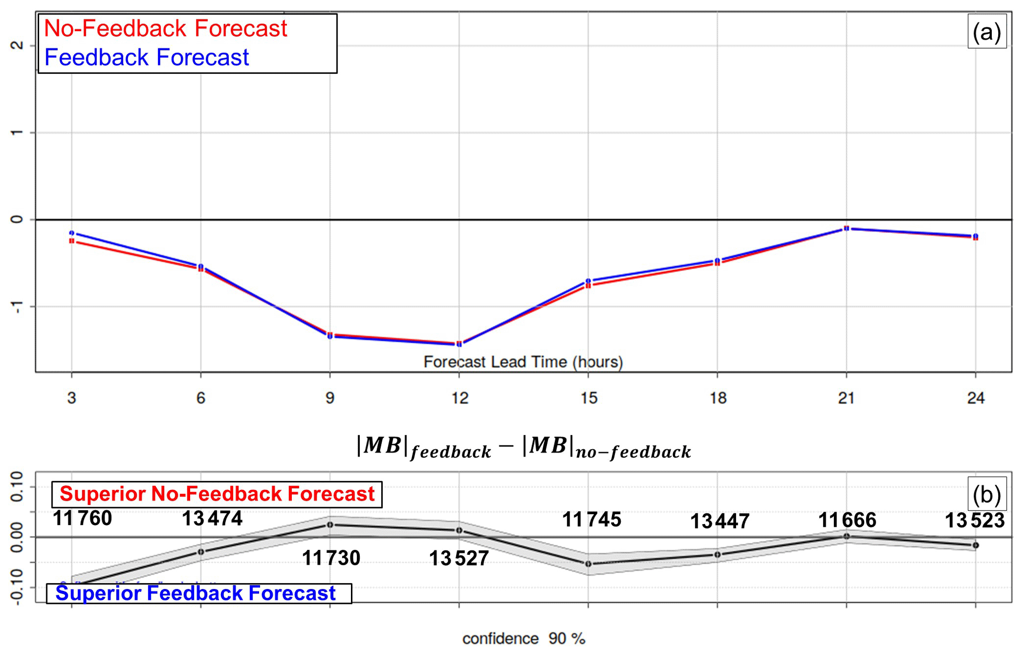
Figure 5Mean bias in surface temperature (^∘C) at forecast hours starting at 00:00 UT. (a) Red line: no-feedback forecast values; blue line: feedback forecast values. (b) Difference in absolute value of mean bias between the two forecasts $\left(\right|\text{MB}{|}_{\text{feedback}}-\left|\text{MB}{|}_{\text{no-feedback}}\right)$, with the region below 90 % confidence level shown shaded grey. Mean values above and below the “0” line and outside of the shaded region thus indicate differences in the mean between the two forecasts which differ at or above the 90 % confidence level. Values of the difference which appear below and above the zero line and outside of the grey area thus indicate superior domain average performance for the feedback/no-feedback forecasts at each of the 3-hourly intervals, respectively. Numbers appearing above the metric differences are the number of observations contributing to the calculated metrics.

Download

Figure 6Summary meteorological performance comparison for surface temperature (^∘C). (a) Mean bias, (b) mean absolute error, (c) root mean square error, and (d) Pearson correlation coefficient. The 90 % confidence level is shown in grey. Numbers appearing above the absolute mean bias differences are the number of stations contributing to the calculated metrics.

Download

Figure 7Summary meteorological performance comparison for surface pressure (hPa). (a) Mean bias, (b) mean absolute error, (c) root mean square error, (d) Pearson correlation coefficient, and (e) standard deviation. The 90 % confidence level is shown in grey. Numbers appearing above the absolute mean bias differences are the number of stations contributing to the calculated metrics.

Download

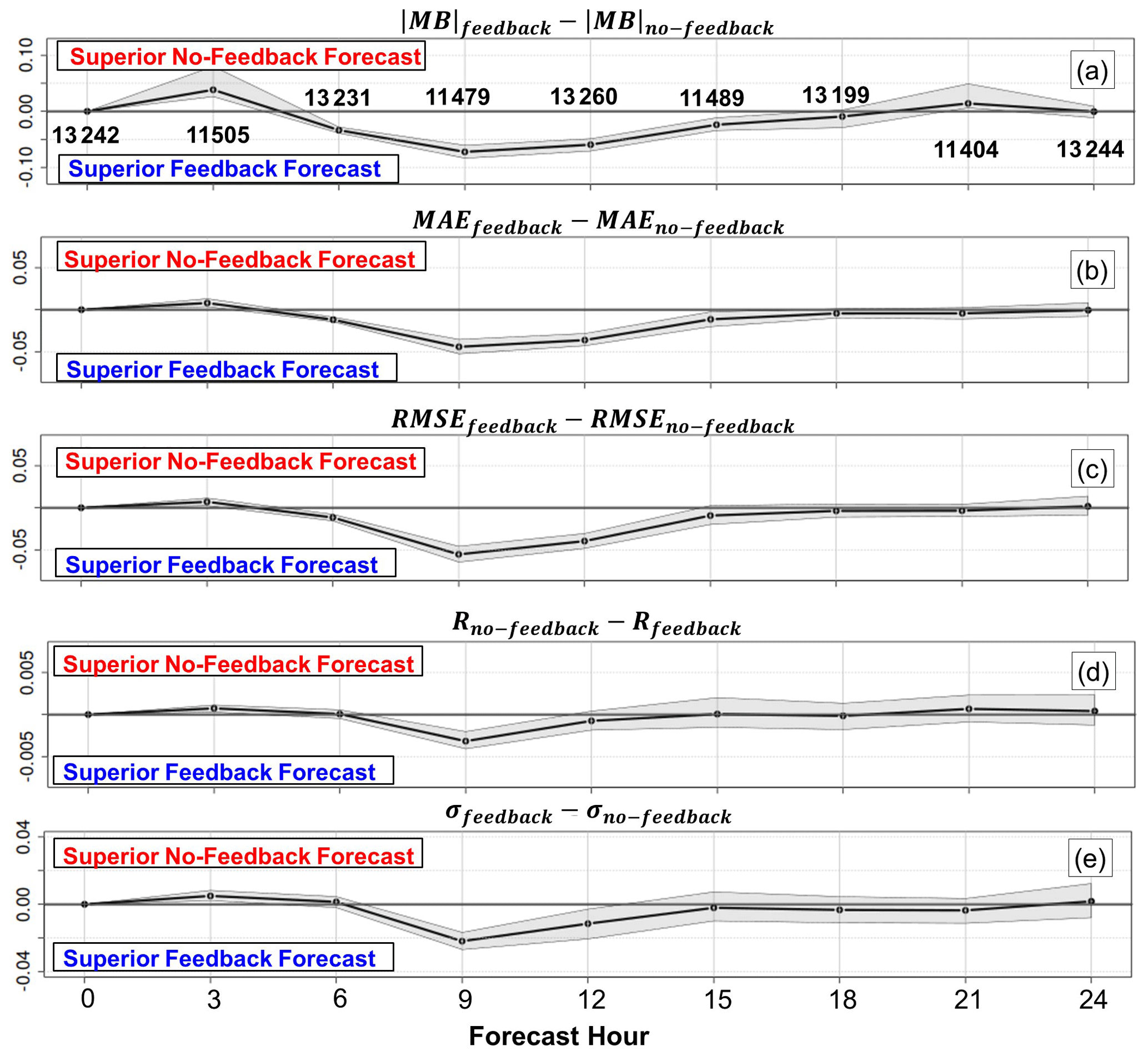
Figure 8Summary meteorological performance comparison for dew-point temperature (^∘C). (a) Mean bias, (b) mean absolute error, (c) root mean square error, (d) Pearson correlation coefficient, and (e) standard deviation. The 90 % confidence level is shown in grey. Numbers appearing above the absolute mean bias differences are the number of stations contributing to the calculated metrics.

Download

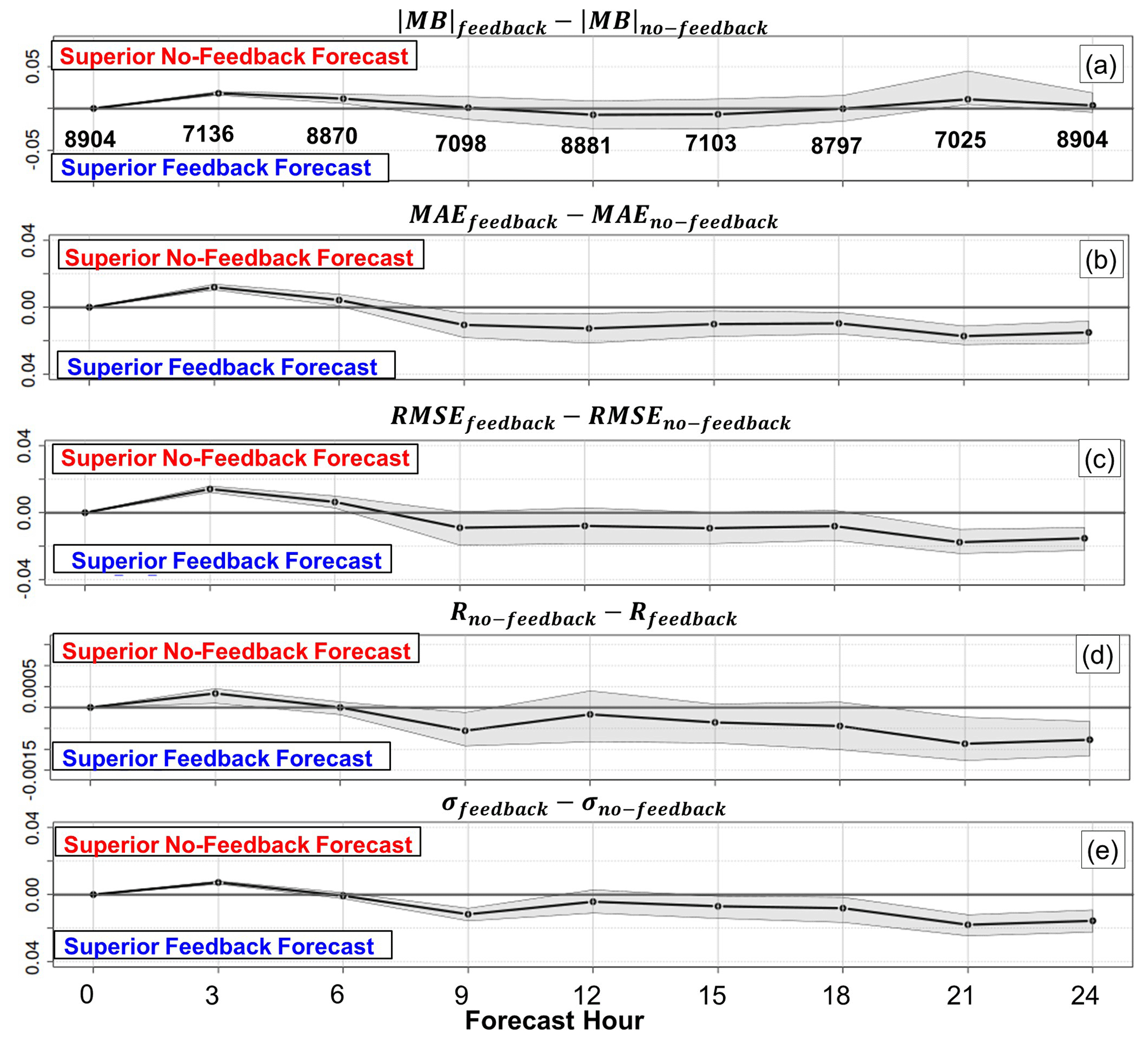
Figure 9Summary meteorological performance comparison for sea-level pressure (hPa). (a) Mean bias, (b) mean absolute error, (c) root mean square error, (d) Pearson correlation coefficient, and (e) standard deviation. The 90 % confidence level is shown in grey. Numbers appearing above the absolute mean bias differences are the number of stations contributing to the calculated metrics.

Download

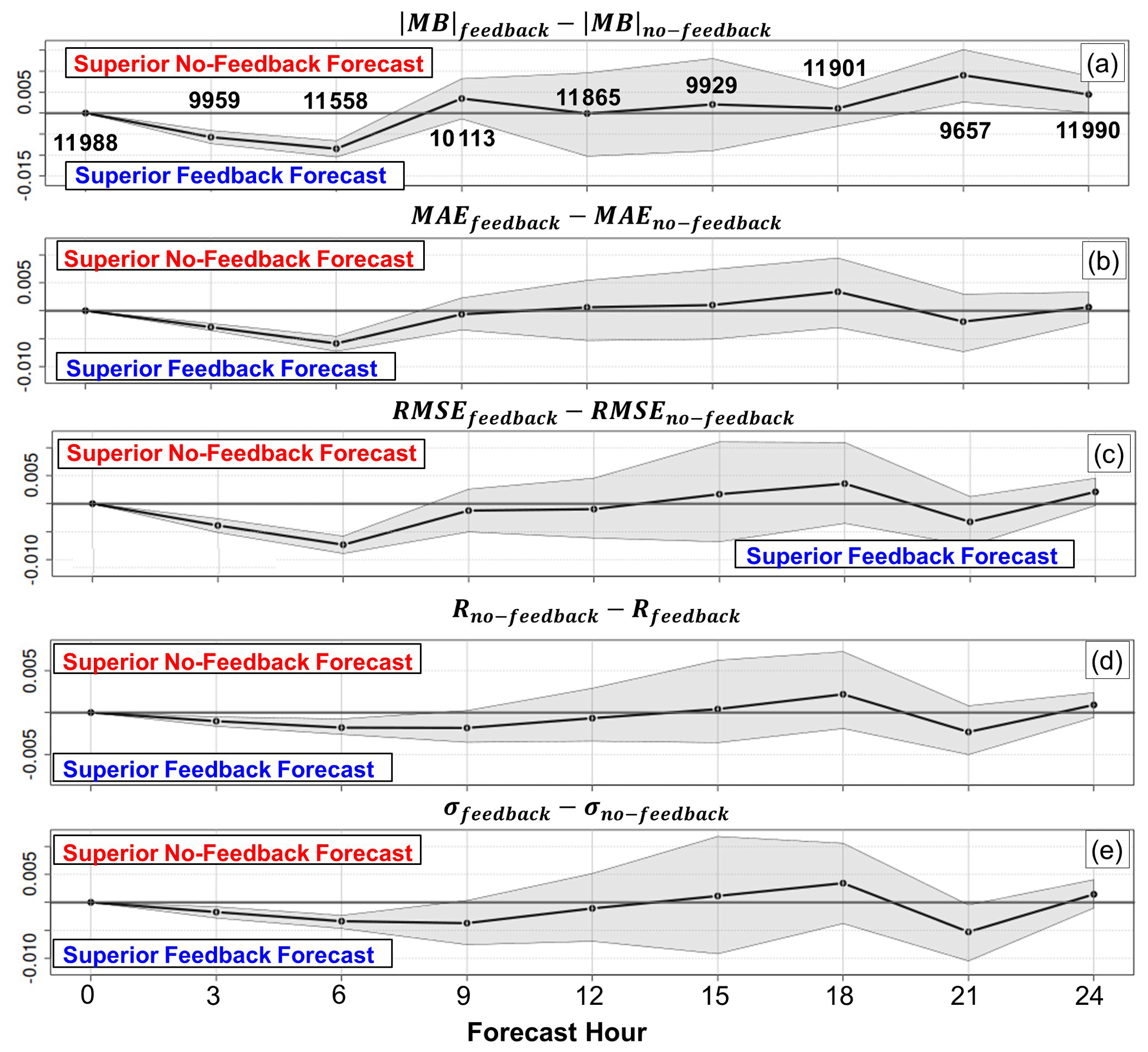
Figure 10Summary meteorological performance comparison for 10 m wind speed (m s⁻¹). (a) Mean bias, (b) mean absolute error, (c) root mean square error, (d) Pearson correlation coefficient, and (e) standard deviation. The 90 % confidence level is shown in grey. Numbers appearing above the absolute mean bias differences are the number of stations contributing to the calculated metrics.

Download

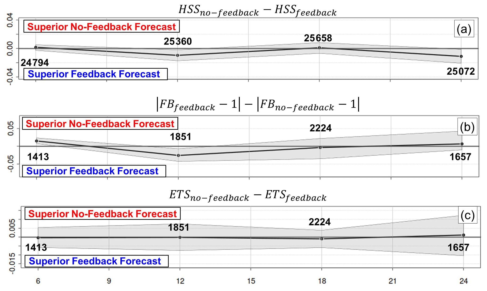
Figure 11Precipitation performance evaluation (mm precipitation). (a) Heidke skill score of 6 h accumulated precipitation (no-feedback–feedback). (b) Frequency bias index of 6 h accumulated precipitation (threshold of 2 mm, no-feedback–feedback). (c) Equitable threat score of 6 h accumulated precipitation (threshold of 2 mm, no-feedback–feedback).

Download

Figure 5 shows an example analysis for surface temperature bias for the entire model domain. Figure 5a shows the average model mean bias (MB) time series across all stations and all forecasts at the given forecast hours, while Fig. 5b shows the corresponding difference in the MB absolute values. The difference plot in Fig. 5b shows the feedback–no-feedback scores, such that scores below the zero line indicate superior performance of the feedback forecast, while those above the zero line indicate superior performance of the no-feedback forecast. Here, the feedback forecast was statistically superior at forecast hours 3, 6, 15, 18, and 24 at the 90 % confidence level at these forecast hours, and both simulations were at par (differences below the 90 % confidence level) at hours 12 and 21, with the no-feedback forecast being superior at 90 % confidence at hour 9. The feedback forecast thus has superior performance, at greater than 90 % confidence, over half of the forecast hours evaluated within the domain, equivalent performance at 2 h (hours 12 and 21, both within 90 % confidence limits), and inferior performance at 1 h (hour 9), during the simulation period.

All of the metrics for which surface temperature forecast performance differed at the 90 % confidence level are shown in Fig. 6. In addition to MB, the scores for MAE and RMSE showed superior forecast performance for the feedback relative to the no-feedback case at the 90 % confidence level for hours 15 and 18, while the improvement for the correlation coefficient only reached the 90 % confidence level at hour 18.

The meteorological forecast performance metrics with statistically significant differences for surface pressure, dew-point temperature, and sea-level pressure are shown in Figs. 7–9 respectively. The model performance differences in these three figures show a similar pattern: a degradation in performance with the use of feedbacks at hour 3, with the differences between the two forecasts either dropping below the 90 % confidence level, or the feedback forecast showing an improvement by hour 9, followed by several hours in which the feedback forecast has a superior performance, usually at greater than 90 % confidence. The duration of this latter period varies between the metrics, from up to 18 h for MAE for surface pressure (Fig. 7b) to 3 h for the correlation coefficient of dew-point temperature (Fig. 8d).

The initial loss of performance for the feedback forecast may represent a form of “model spin-up” that may be unique to online coupled models but may be affected or improved with further adjustments to the forecast cycling setup for the chemical species. As noted earlier (Fig. 2), in order to prevent chaotic drift from observed meteorology, we made use of a 30 h 2.5 km resolution analysis-driven weather forecast to update our online coupled model's initial meteorology at hour zero of each 24 h forecast. The cloud fields provided as initial conditions at hour zero include observation analysis for the 6 h prior to hour zero – these have reached a quasi-equilibrium in the high-resolution weather forecast (Fig. 2b and e) by the time they are used as initial and boundary conditions in the online coupled model (Fig. 2c and f). However, the online coupled model's aerosol fields at hour zero, used to initialize the subsequent forecast (Fig. 2, dashed blue arrow), still reflect the locations of aerosol–cloud interactions in the previous online coupled simulation. The initial 3 to 6 h of feedback forecast degradation represents the time required for the online coupled model to reach a new equilibrium consistent between both its aerosol and the cloud fields.

One possible solution for this model spin-up inconsistency would be to eliminate the intermediate driving 2.5 km meteorological simulation in favour of a longer 30 h online coupled forecast with the first 6 h removed as spin-up (i.e., extend the duration of steps c and f in Fig. 2 to 30 h, starting at UT hour 6). The duration of the forecast experiments carried out here was limited to 24 h due to limited computational resources and, more importantly, to the operational requirement for an on-time forecast delivery for the purpose of the FIREX-AQ field campaign. The 24 h forecast simulations carried out in Fig. 2c and f each required nearly 3 h of supercomputer processing time; longer simulation periods were not possible within the operational window available for forecasting.

Model 10 m wind speed forecasts were also improved with the incorporation of feedbacks for hours 3 and 6, for all metrics (Fig. 10). A decrease in MB performance at hours 21 and 24 can also be seen in this figure.

Precipitation forecast performance from the two simulations varied depending on the metric chosen (Fig. 11). The metrics in this case were based on the number of coincident precipitation “events” versus “non-events” as shown in Table 2.

Table 2Event versus non-event contingency table. A is the number of events forecast and observed; B is the number of events forecast but not observed; C is the number of events observed but not forecast; D is the number of cases where events were neither forecast nor observed.

Download Print Version | Download XLSX

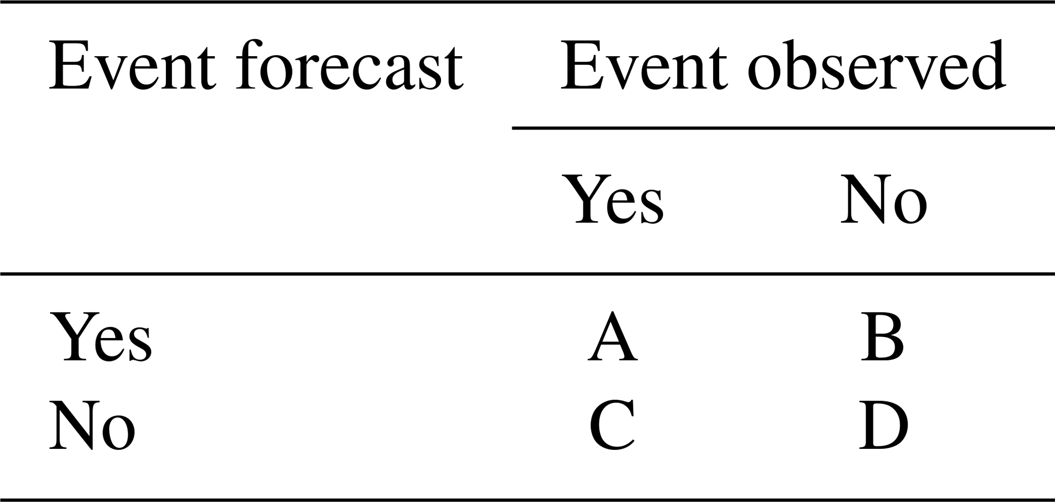
The Heidke skill score $\mathit{\{}\text{HSS}=\mathrm{2}(AD-BC)/[(A+C)(C+D)+(A+B)(B+D)\left]\mathit{\right\}}$ measures the fractional improvement of the forecast over the number correct by chance. The frequency bias $\mathit{\{}\text{FB}=(A+B)/(A+C\left)\mathit{\right\}}$ measures the frequency of event over-forecasts (FB > 1) versus event under-forecasts (FB < 1). The equitable threat score $\mathit{\{}\text{ETS}=(A-\stackrel{\mathrm{̃}}{A})/(A+C+B-\stackrel{\mathrm{̃}}{A})$, where $\stackrel{\mathrm{̃}}{A}=(A+B)(A+C)/(A+B+C+D)\mathit{\}}$ measures the observed and/or forecast events that were correctly predicted. Following standard practice at Environment and Climate Change Canada, the HSS is used as a measure of total precipitation accumulated over a 6 h interval, with no lower limit on the amount of precipitation defining an event, while FB and ETS define precipitation events as being those with greater than 2 mm per 6 h interval – consequently FB and ETS have a smaller number of data points for comparison than HSS.

Figure 11 shows that improvements to the online coupled precipitation forecast at the 90 % confidence level were seen for the HSS 6 h accumulated metric at hours 12 and 24, while the frequency bias index of 6 h accumulated precipitation showed degradation at hours 6 and improved performance at hour 12, and the equitable threat score of 6 h accumulated precipitation showed significant differences at 90 % confidence between the two simulations. As is noted above, the latter two metrics employed a minimum 6 h precipitation threshold of 2 mm prior to comparisons (this is the reason for the reduced number of points available for comparison in Fig. 11b and c relative to Fig. 11a). These findings suggest that the online coupled model's improvements for total precipitation (Fig. 11a) are the result of slightly improved performance for relatively light precipitation events (<2 mm 6 h⁻¹).

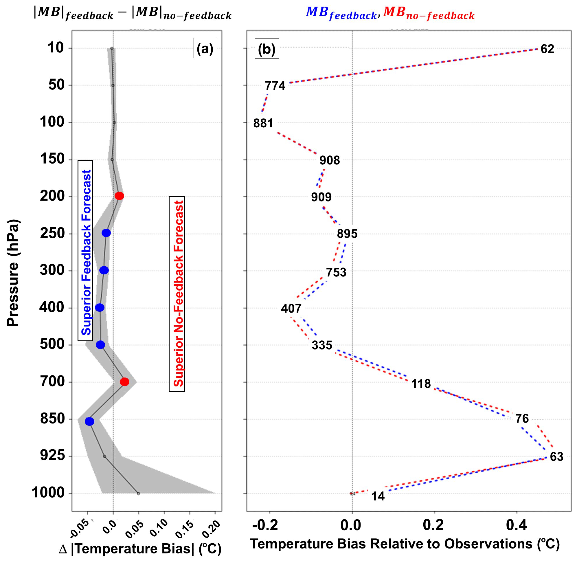
Figure 12Forecast hour 12 (00:00 UT) summary upper air temperature performance comparison for air temperature (mean bias, ^∘C). (a) Difference in absolute value of mean bias in temperature (feedback forecast–no-feedback forecast). Grey regions represent 90 % confidence levels, and blue symbols show pressure levels at which the feedback mean bias outperforms the no-feedback mean-bias at >90 % confidence. Red symbols show pressure levels at which the no-feedback mean bias outperforms the feedback mean bias at >90 % confidence. The 90 % confidence level is shown in grey. (b) Mean bias in upper air temperature for feedback (blue) and no-feedback (red) (^∘C). Numbered values on the profiles indicate the number of observed data–model pairs at each pressure level.

Download

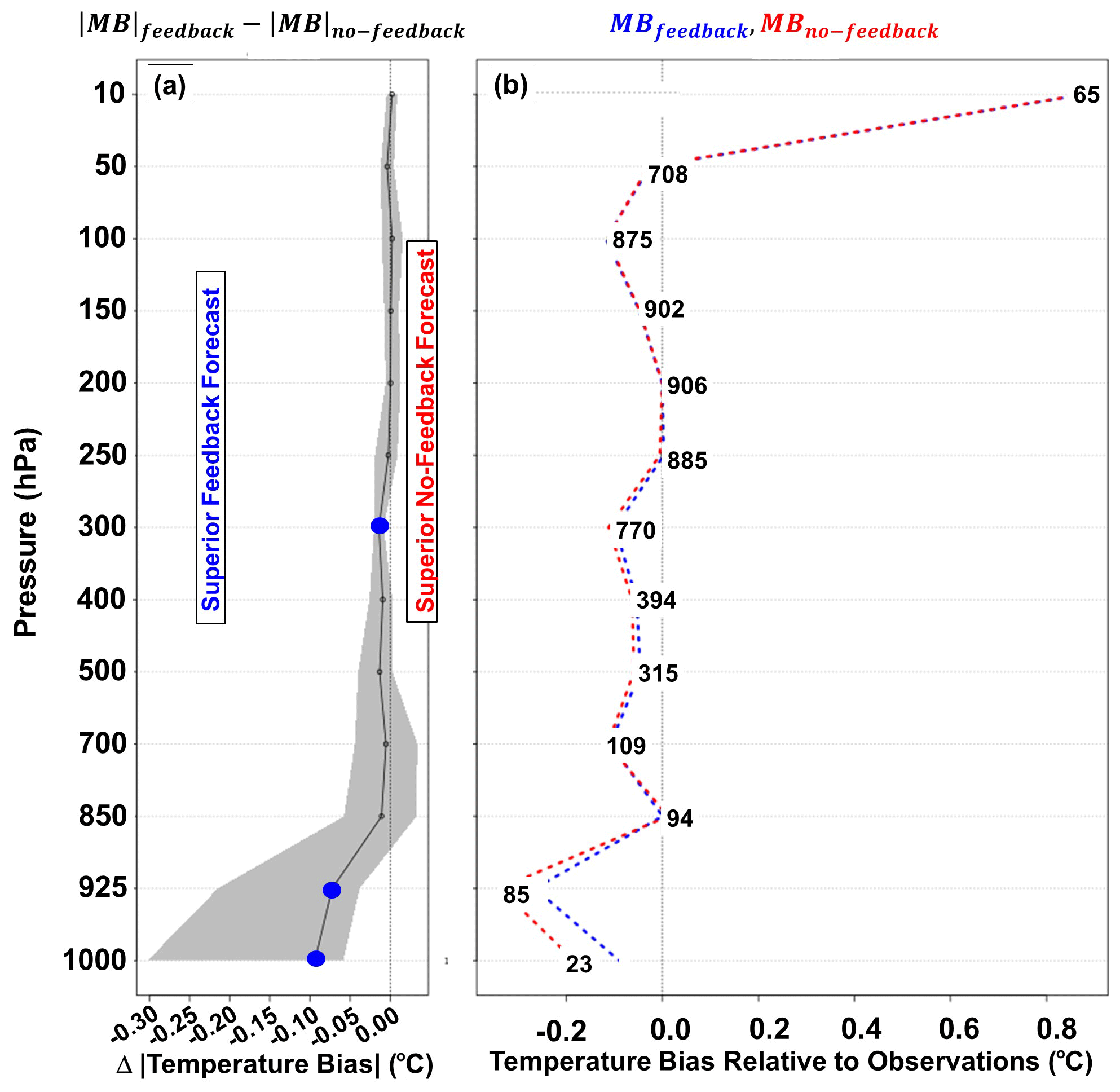
Figure 13Forecast hour 24 (12:00 UT) summary upper air temperature performance comparison for air temperature (mean bias, ^∘C). (a, b) as in Fig. 12.

Download

The amalgamated observations and model pairs of vertical temperature profile data from 39 radiosonde sites in western North America are shown in Figs. 12 and 13. Improvements in the forecasted temperature vertical profile with increasing forecast time are evident at 250, 300, 400, 500, and 850 hPa in the 12th hour forecast, with degradations at 200 and 700 hPa (Fig. 12). Improvements at 300, 925, and 1000 hPa may be seen in the 24th hour (Fig. 13) forecast; it is also worth noting that the entire region at and below 300 hPa has improved temperature forecasts (mean values to the left of the vertical line), albeit not always at >90 % confidence. There are larger differences between the 1000 hPa forecasts, though these also have the least number of contributing stations (i.e., only those located close to sea level contribute to the lowest level temperature biases). Other levels of the atmosphere showed no statistically significant change at the 90 % confidence level in temperature profile forecast performance with the use of feedbacks.

3.2 Chemistry evaluation

Improvements to air-quality model performance metrics have been a focus for research since the 1980s, starting with dispersion model evaluation (Fox, 1981) and the identification of mean bias and normalized mean square error as potentially useful metrics to complement the Pearson correlation coefficient (Hanna, 1988). More recently, the Pearson correlation coefficient has been noted as being capable of producing high values for relatively poor model results (Krause et al., 2005), as well as being unable to distinguish systematic model underestimation (Yu et al., 2006), unable to provide information on whether data series have a similar magnitude, and capable of providing a false sense of relationship where none exists due to outliers (Duveiller et al., 2016) and clusters of model–observation pairs (Aggarwal and Ranganathan, 2016). More recently, model evaluation has focused on metrics which do not have the tendency to weight the higher magnitude values unduly (a particularly useful property with air-quality variables, which may vary by several orders of magnitude), which are dimensionless (allowing a comparison across different evaluated variables) and which are bounded and symmetric (properties allowing comparisons to be made and equally valued across the entire range of possible concentrations; e.g., Yu et al., 2006). Metrics such as the modified coefficient of efficiency (Legates and McCabe, 1999) and the more recent incarnations of the index of agreement (Willmott et al., 2012) are examples of the more recent metrics used for air-quality model evaluation. Here, we have made use of a range of metrics spanning the literature on this topic, with the understanding that the properties of different metrics vary, that no single metric provides a perfect means of evaluating model performance, and that a variety of metrics should be applied. The metrics used here span the variety that have appeared in the literature since the early 1980s and include the factor of 2, mean bias, mean gross error, normalized mean gross error, correlation coefficient, root mean square error, coefficient of efficiency, and index of agreement. The formulae for these metrics and a brief description of their relative advantages and disadvantages appear in Sect. S1 and Table S1 in the Supplement.

Table 3Summary performance metrics for ozone, nitrogen dioxide, and PM_2.5. Boldface indicates the simulation with the better performance score for the given metric, chemical species, and subregion, italics indicate a tied score, and regular font indicates the simulation with the lower performance score. FO2: fraction of scores within a factor of 2. MB: mean bias. MGE: mean gross error. NMGE: normalized mean gross error. R: correlation coefficient. RMSE: root mean square error. COE: coefficient of error. IOA: index of agreement.

Download Print Version | Download XLSX

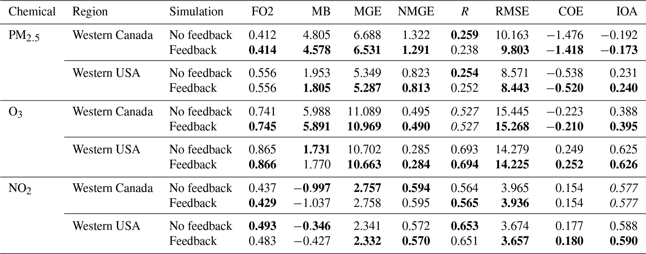
Both simulations' performance for ozone (O₃), nitrogen dioxide (NO₂), and particulate matter with diameters less than 2.5 µm (PM_2.5) were evaluated using the above metrics, employing hourly AIRNOW data (for USA, AQS network: https://www.epa.gov/aqs, 17 June 2021; for Canada, NAPS network: http://maps-cartes.ec.gc.ca/rnspa-naps/data.aspx, 17 June 2021) and the openair package (Carslaw and Ropkins, 2012). The summary performance metric scores for the two simulations grouped, according to contributing measurement network, are shown in Table 3, with boldfaced values indicating the better score for the given simulation case. With respect to this table, we note the following:

• a.

  The feedback simulation generally outperforms the no-feedback simulation (more boldfaced scores in the feedback rows, for 35 out of 48 metric comparisons).

• b.

  Feedback forecast score improvements occurred were more noticeable for PM_2.5 (usually first to second digit), followed by O₃, with the NO₂ scores often being the same for the first few digits.

• c.

  We note that the boundary conditions employed for our 2.5 km simulations had a strong impact on model air-quality performance. As described above, these boundary conditions originated in a 10 km resolution simulation making use of ECMWF global reanalysis values on its own lateral boundaries. The magnitudes of the statistics of Table 3 may be compared to the magnitudes of the statistics from our initial ACPD submission (which made use of a MOZART 2009 reanalysis for chemical lateral boundary conditions for the 2.5 km GEM-MACH domain); these earlier results are shown in the Supplement, Table S2. The use of feedbacks had a similar relative impact on forecast performance (34 out of 48 statistics improving in the feedback forecast in the initial simulation, compared to 35 out of 48 statistics in the current work). However, the net impact of the ECMWF-driven 10 km GEM-MACH values being used for chemical lateral boundary conditions, rather than the MOZART climatology, was a degradation of performance: comparing the equivalent entries in Tables 3 and S2, it can be seen that 71 out of 96 scores were better with the earlier use of the MOZART reanalysis. As we show below, however, the revised boundary conditions led to improvements in model aerosol optical depth performance relative to observations.

The impact of lateral boundary conditions on model predictions can be seen when comparing MODIS retrievals of aerosol optical depth (AOD) with model predictions (Fig. 14). AOD is a function of both the particle's abundance and optical properties, integrated throughout the vertical column. However, direct comparisons between satellite and model-predicted AOD values must be undertaken with some care, due to the nature of the satellite retrieval quality assurance and control procedures, the motion of the orbiting spacecraft, and the scan time of the instrument. The manner in which AOD is calculated introduces additional uncertainty due to the range of values which may be derived from the same aerosol speciation using different methodologies (Curci et al., 2015). For a polar-orbiting instrument such as MODIS, the time at which overpasses occur varies with location, and valid satellite retrievals may not occur when the location being scanned is obscured by clouds. Observed averages may be built up over multiple valid scans over time, but the number of valid scans contributing to the local average at any given location will vary, due to the time and space variation in cloud cover. Here, individual valid Collection 6.1 MODIS/Aqua (MYD04_L2 AOD_550_Dark_Target_Deep_Blue_Combined) 10 km resolution 550 nm AODs were matched in time and space to the nearest model 2.5 km grid cell and output frequency hour. The paper by Levy et al. (2013) contains details on the MODIS combined AOD product. No averaging was employed in our comparison (Fig. 14); all satellite overpass AOD pixels and matching model AOD pixels are shown. Noting that the AOD colour scale is logarithmic, the model simulation driven using the ECMWF + 10 km resolution GEM-MACH for boundary conditions (Fig. 14b) is a much better match to observations (Fig. 14a) than the model simulation driven by MOZART climatological boundary conditions (Fig. 14c). The slope of the linear best fit line between all observation and model pairs in each case mirrors this finding, with the original (MOZART climatology) boundary conditions having a slope of 0.15 and R² of 0.0382 and the revised ECMWF + GEM-MACH 10 km boundary conditions having a slope of 0.56 and an R² of 0.067.

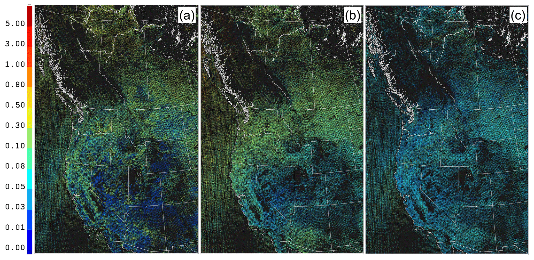
Figure 14550 nm AOD comparison. (a) All MODIS observations sampled over the model domain and forecast duration and (b) GEM-MACH 2.5 km simulation, driven by 10 km GEM-MACH simulations, in turn driven by ECMWF reanalysis for 2.5 km domain boundary conditions. (c) GEM-MACH 2.5 km simulation, driven by MOZART climatological boundary conditions.

Previous work with CFFEPS by Chen et al. (2019) for the 2017 fire season has shown similar PM_2.5 positive biases for western Canada, with MB of +5.8 µg m⁻³ (88 stations) and for western USA with MB of +8.6 µg m⁻³ (221 stations). These positive biases (Chen et al., 2019) were higher specific to subregions closer to areas of active fires (MB of +12 µg m⁻³ for the subregion including the provinces of Alberta and British Columbia and +29 µg m⁻³ for the subregion comprising the states of Idaho, Montana, Oregon, and Washington, respectively). At least part of the positive biases may be due to 10 km GEM-MACH forest-fire emissions occurring in the state of Alaska being overestimated during the study period. However, the ECMWF reanalysis also captures significant particulate mass crossing the Bering Strait from fires in Siberia during this period, so the relative contributions of fires within the low-resolution GEM-MACH domain and the ECMWF boundary conditions driving that domain are combined and cannot be separated in the runs carried out here.

The local AOD positive biases associated with fires could also be the result of the mixing state assumptions of the Mie code used here for generating aerosol optical properties. These assumptions may also account for negative AOD biases over much of the remainder of the model domain. As noted earlier, this overall negative bias of AOD predictions (both boundary condition configurations result in observation:model slopes less than unity) is a common problem in air-quality models and may be due to assumptions regarding the model mixing state (Curci et al., 2015). That comparison of multiple mixing state assumptions on AOD with observations for European and North American modelling domains (Curci et al., 2015) showed a typical factor of 2 model underprediction of 440 nm North American AOD across all mixing state assumptions, with European AOD negative biases ranging from unbiased to a factor of 2. These earlier findings along with overestimates at forest-fire plumes with our current homogeneous mixture approach at 550 nm suggest that the hygroscopic growth may be overestimated for forest-fire particles, in turn overestimating forest-fire AODs locally, while external mixing assumptions may be required to improve model AOD performance elsewhere in the model domain.

We note that the combined use of the ECMWF global reanalysis and a 10 km resolution GEM-MACH simulation to provide boundary conditions for our 2.5 km domain resulted in a degradation of model performance for surface PM_2.5, O₃, and NO₂, for 71 out of 96 statistical scores, compared to the use of a MOZART2009 reanalysis for 2.5 km domain boundary conditions. The improvement associated with the use of feedbacks was maintained, showing that the impact of feedbacks is a robust finding. However, the performance degradation associated with the change of boundary conditions is a source of concern.

We also note that, while AOD performance has improved with the use of the ECMWF + GEM-MACH 10 km boundary conditions in Fig. 14, significant overestimates of AOD occur with the use of these boundary conditions, in several regions in the USA. This may be seen by comparing Fig. 14a and b for the states of Montana, Wyoming, Nevada, New Mexico, and Utah, where the dark blue colours in the observations (Fig. 14a) indicate observed AODs less than 0.01, whereas the 10 km simulations driven by ECMWF + GEM-MACH (Fig. 14b) indicate values of 0.03 to 0.05). This is consistent with the increase in positive surface bias in PM_2.5 associated with the use of the ECMWF + GEM-MACH 10 km boundary conditions (e.g., feedback runs having western Canada and western USA positive biases of PM_2.5 of 4.578 and 1.805 µg m⁻³ (Table 1), compared to the MOZART2009 reanalysis driven run values of 0.236 and −1.786 µg m⁻³ (Table S2), respectively). The boundary condition setup thus accounts for a substantial increase in overall surface PM_2.5 mass, with the use of ECMWF + GEM-MACH 10 km increasing mean PM_2.5 by 4.34 and 3.59 µg m⁻³ in western Canada and USA, respectively, relative to the use of MOZART2009.

The reduction in performance may thus be due to two possible causes (or their combination): (1) the domain within the GEM-MACH 10 km simulation might be sufficiently large, and the emissions in the regions between the 10 km boundaries and the 2.5 km domain sufficiently in error, that the 2.5 km simulation accuracy is adversely affected; (2) the ECMWF reanalysis employed on the outermost boundary of the 10 km domain contributes sufficient PM_2.5, NO₂, and O₃ to the simulations that the innermost domain model performance at the surface is adversely affected. That is, the degradation in performance may be associated with the GEM-MACH 10 km simulation, the ECMWF reanalysis, or a combination of both factors.

In order to examine the potential impact of the ECMWF reanalysis used as the outermost domain boundary conditions, we evaluated the ECMWF reanalysis using the same observation data, station locations, and performance metrics as were used for our 2.5 km simulations – the results of this analysis are shown in Tables S3 (PM_2.5), S4 (O₃), and S5 (NO₂). This additional analysis shows that the ECMWF reanalysis values during the study period have higher positive biases for PM_2.5 and O₃ and lower negative biases for NO₂ than the corresponding 2.5 km GEM-MACH simulations. A similar pattern occurs for the other statistical metrics, with the ECMWF reanalysis usually having a reduced performance for most statistical scores for PM_2.5, O₃, and NO₂ over the study region in comparison to the high-resolution model simulations carried out here. The ECMWF reanalysis was also evaluated for the same time period for the entire North American domain, in Tables S3 to S5; the scores for this last analysis suggest that the performance of the reanalysis relative to observations is similar over the continent and is not limited to our study area. We note that the ECMWF reanalysis has relatively low spatial and time resolution compared to the 2.5 km simulations carried out here ($\mathrm{0.75}{}^{\circ }\times \mathrm{0.75}{}^{\circ }$ versus 2.5 km×2.5 km, 3-hourly output values compared to 1 h output values) and relatively coarse resolution for particle sizes (e.g., 3 size bins compared to the 12 bins used within GEM-MACH; these issues may factor into the performance scores). The comparison does not rule out the possibility that GEM-MACH's 10 km resolution simulations may also contribute adversely to our 2.5 km model performance. However, our analysis suggests that our use of the ECMWF reanalysis for boundary conditions on our outermost domain likely accounts for at least some of the performance degradation in our modelling system, compared to the MOZART2009 boundary condition simulation carried out earlier.

3.3 Model evaluation summary

Overall, the incorporation of feedbacks in this study has resulted in improvements in weather and air-quality forecast accuracy, albeit with some caveats. Weather forecast variables showed improvements at the 90 % confidence level for several fields, and vertical profiles showed a matching performance or improvements at most levels and times. Total precipitation scores also showed minor improvements or matching performance at the 90 % confidence level. A previously unexpected spin-up issue specific to online coupled models was noted: the impact of online coupled particulate matter on cloud variables was sufficiently strong that cloud field adjustment in the first 6 h of the forecast was required prior to some weather forecast variable improvements to be apparent (surface pressure, dew-point temperature, sea-level pressure). While the current forecast cycling duration was constrained by operational requirements, this suggests that forecast cycling should include both air-quality and meteorological variables during online coupled forecast spin-up periods. That is, the model tracer concentrations 6 h prior to the current forecast start-up could also be used during the initial meteorological spin-up period, thus allowing for the simultaneous spin-up of chemistry and cloud formation. Scores for surface PM_2.5, NO₂, and O₃ also generally improved with the incorporation of feedbacks (35 out of 48 comparisons showed improvements). The choice of lateral boundary conditions was shown to have a significant impact on chemical performance within the model domain. In comparison to satellite-based AOD values, the current model's AOD values were generally biased low, with smaller magnitude biases being associated with the ECMWF + 10 km GEM-MACH boundary conditions. The latter comparison also showed that large fires off-domain in Alaska and Siberia likely had a large impact on AODs in the eastern and northern section of the model domain, through comparison with our initial simulations.

4.1 Effects of feedbacks on time-averaged meteorology

The feedback–no-feedback differences in the simulation-period average cloud droplet number density (number per kilogram of air) and mass density (grams of water per kilogram of air) along centered cross sections spanning the length and width of the 2.5 km resolution model domain are shown in Fig. 15 (cross section locations are shown in Fig. 1). The “ocean”, “land”, and “forest fire” regions identified are with reference to the approximate locations of these features along these cross sections. Figure 15 also shows the confidence ratio values as described above – regions where the predicted mean values differ at or above the 90 % confidence level are shown in red, while those differences below the 90 % confidence interval are shown in blue. Feedbacks increase the cloud droplet number density over the northern part of the domain, including the region impacted by the Alberta–Saskatchewan forest fires, from the surface up to about 500 mb (roughly equivalent to hybrid level 0.500), and decrease at higher elevations further to the south and along the length of the model domain into the western USA (Fig. 15a). Cloud droplet numbers also decrease over the ocean but increase eastwards over the land (Fig. 15b). The latter is unrelated to the forest fires; this is an indication that the modelled aerosol number concentration over the ocean is much lower than the single climatological aerosol population assumed in the no-feedback run, resulting in lower cloud droplet number concentrations. The changes are significant at the 90 % confidence level from the surface up to hybrid level 0.60 in the northern region which is most impacted by forest-fire smoke, and in isolated regions further aloft along the south–north cross section (Fig. 15c), and over the regions of the ocean in the west–east cross section (Fig. 15d). Aerosol loadings that are higher than climatology, a large portion of which are due to the forest fires, resulted in increased cloud droplet number densities in the lower troposphere while decreasing them in the middle–upper troposphere (Fig. 15a). This impact of feedbacks is in accord with the satellite observations of Saponaro et al. (2017) and was also seen in Takeishi et al. (2020). In contrast, cloud droplet mass density (i.e., cloud liquid water content) largely decreases across the domain along the north–south cross section (Fig. 15e), as well as over the ocean, with a varying pattern over the land in the east–west cross section (Fig. 15f). The magnitudes and significance levels for the average change in cloud droplet mass are lower than for cloud droplet number, with the most significant differences occurring over the ocean (Fig. 15g and h).

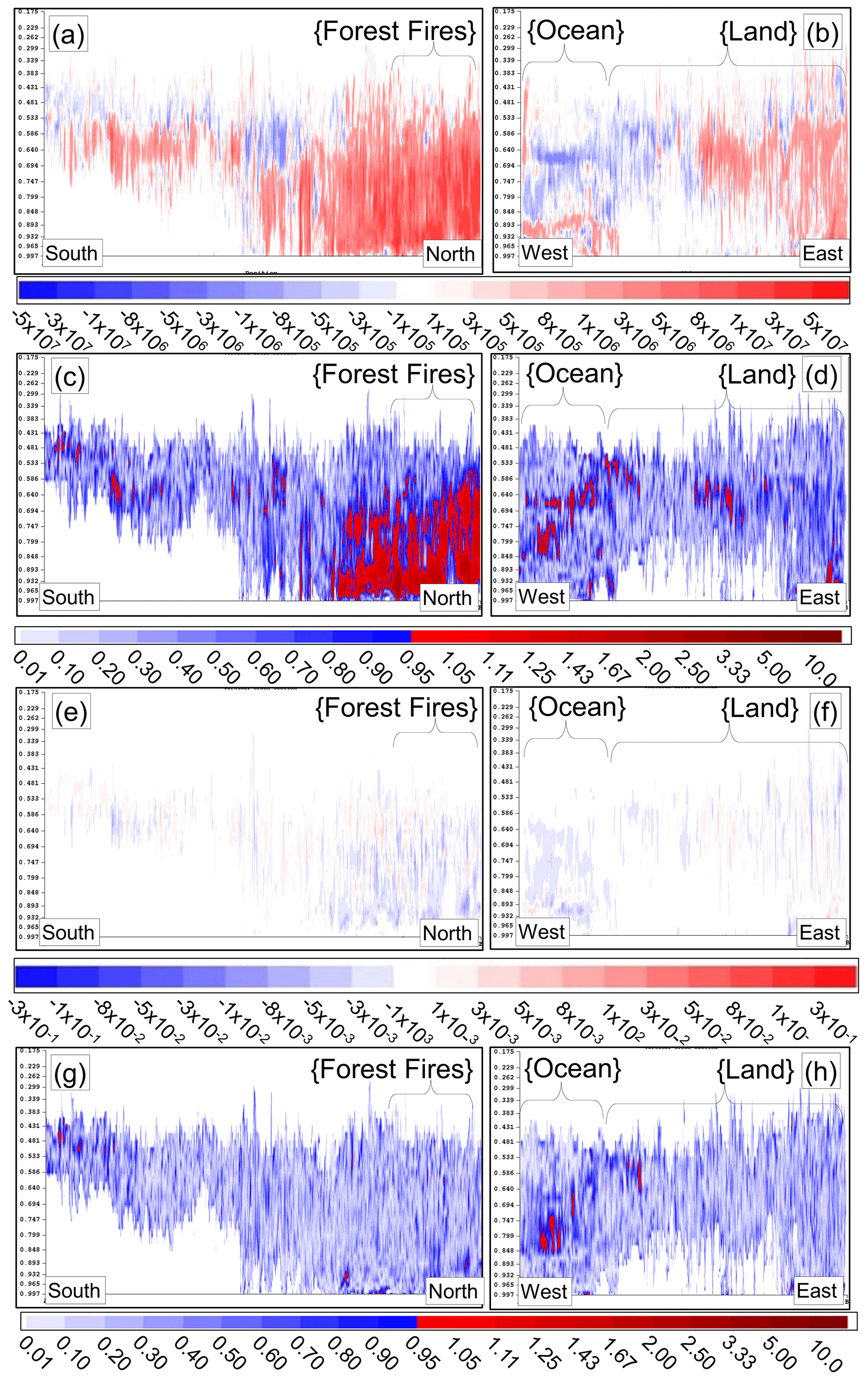
Figure 15(a, b) Difference in mean (feedback–no-feedback) cloud droplet number simulations along south–north and east–west cross sections through the middle of the model domain. (c, d) Corresponding significance level of mean cloud droplet number differences using the confidence ratio defined in Eq. (S1) in Sect. S2 – red areas indicate ratio values greater than unity, i.e., significance at or above the 90 % confidence level. (e, f) Difference in mean cloud droplet mass (g kg⁻¹). (g, h) Corresponding significance level of mean cloud droplet mass difference. Note: the vertical axis in hybrid coordinates does not show all model levels for clarity; the model has much finer resolution in the lower part of the atmosphere than shown, and the portion of the vertical domain shown encompasses only the lower half of the levels in the model.

Download

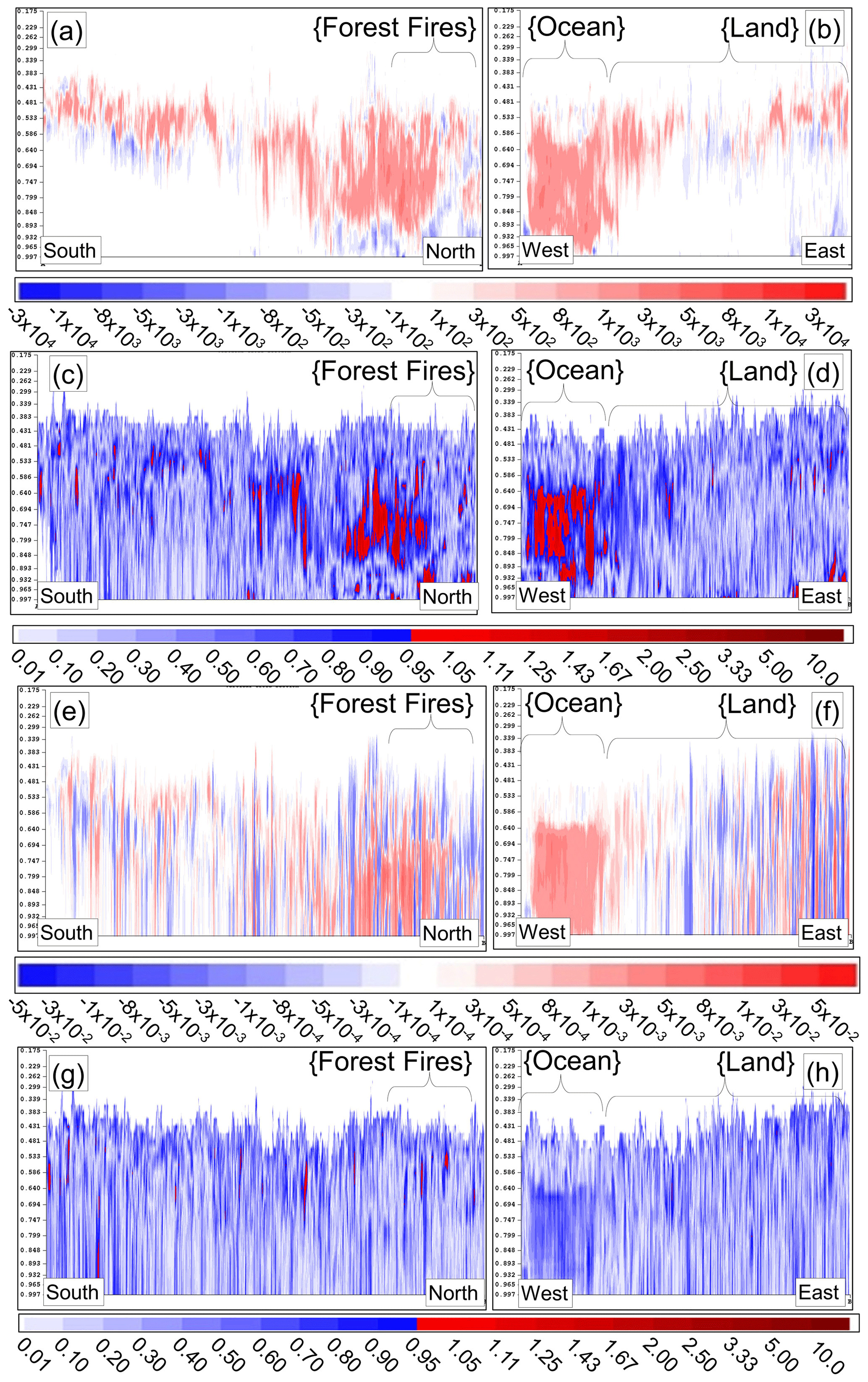
Figure 16(a, b) Difference in mean (feedback–no-feedback) raindrop number simulations along south–north and east–west cross sections through the middle of the model domain. (c, d) Corresponding significance level of mean raindrop number differences using the confidence ratio defined in Eq. (S1) in Sect. S2 – red areas indicate ratio values greater than unity, i.e., significance at or above the 90 % confidence level. (e, f) Difference in rain cloud drop mass (g kg⁻¹). (g, h) Corresponding significance level of mean raindrop mass difference.

Download

Consistent with the cloud droplet number changes, rain droplet numbers and mass mixing ratios increase aloft with the feedback simulation, over both the forest region impacted by the forest fires (Fig. 16a and e) and over the ocean (Fig. 16b and f), with a varying impact over the land and more distant from the forest-fire sources (Fig. 16f). The changes are significant at the 90 % confidence level for rain droplet number in these regions (compare Fig. 16a with c; 16b with d), while the rain droplet mass changes sometimes reach but are usually below the 90 % confidence level (Fig. 16g and h).

These results suggest that relative to the no-feedback simulation, which employs climatological aerosol CCN properties, the AIE in the feedback simulation is causing significant change in hydrometeor numbers and a less significant increase in hydrometeor mass. In the forest-fire-impacted region, the ADE and AIE in the feedback simulation significantly increase the number of cloud droplets near the surface and throughout the middle to upper troposphere (Fig. 15a and c). The raindrop number in the middle troposphere (Fig. 16a and c) also increases significantly between hybrid levels 0.90 and 0.70 (Fig. 16e and g). Near-surface raindrop number and raindrop mass differences throughout the cross sections (Fig. 16e and f) fall below the 90 % confidence level (Fig. 16g and h).

Over the oceans, water droplet number and mass both decrease (Fig. 15b and f), and raindrop number and mass increase (Fig. 16b and f); more atmospheric water is converted to raindrops as a result of the feedbacks, relative to the climatology in the no-feedback simulation. However, these changes are more significant aloft than at the surface, with the difference in both raindrop number and mass falling below the 90 % confidence level near the surface. We interpret these changes as a shift in over-ocean liquid hydrometeor numbers and to a lesser degree the water mass aloft from cloud droplets to raindrops due to the AIE in the feedback setup relative to the climatology of the no-feedback simulation. The changes occur at the 90 % confidence level aloft, but the near-surface changes are smaller and are usually below the 90 % confidence level.

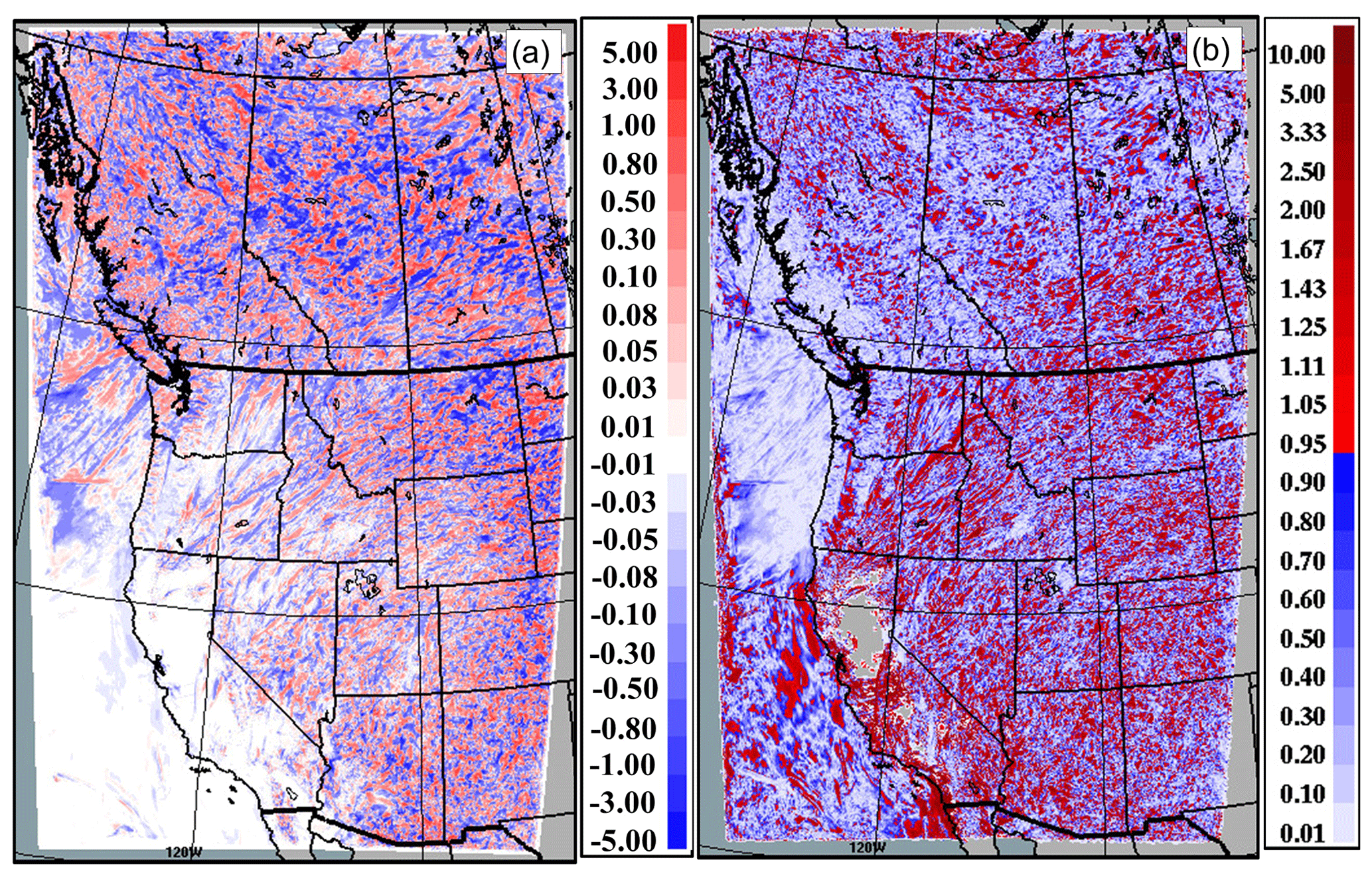
Figure 17(a) Average (feedback–no-feedback) total surface precipitation during the simulation period. (b) The 90 % confidence ratio – values greater than 1 indicate significantly different results at the 90 % confidence level.

Differences in the average surface precipitation flux and the confidence ratio values are shown in Fig. 17. Changes in average precipitation (Fig. 17a) appear random, though locally these differences are significant at the 90 % confidence level (Fig. 17b). Both the magnitude of the differences and the frequency in their reaching the 90 % confidence level increase south-westwards. Given the local and episodic nature of rainfall events, the high level of significance in this case probably results from the presence or absence of individual rainfall events between the two simulations affecting the local average and standard deviations.

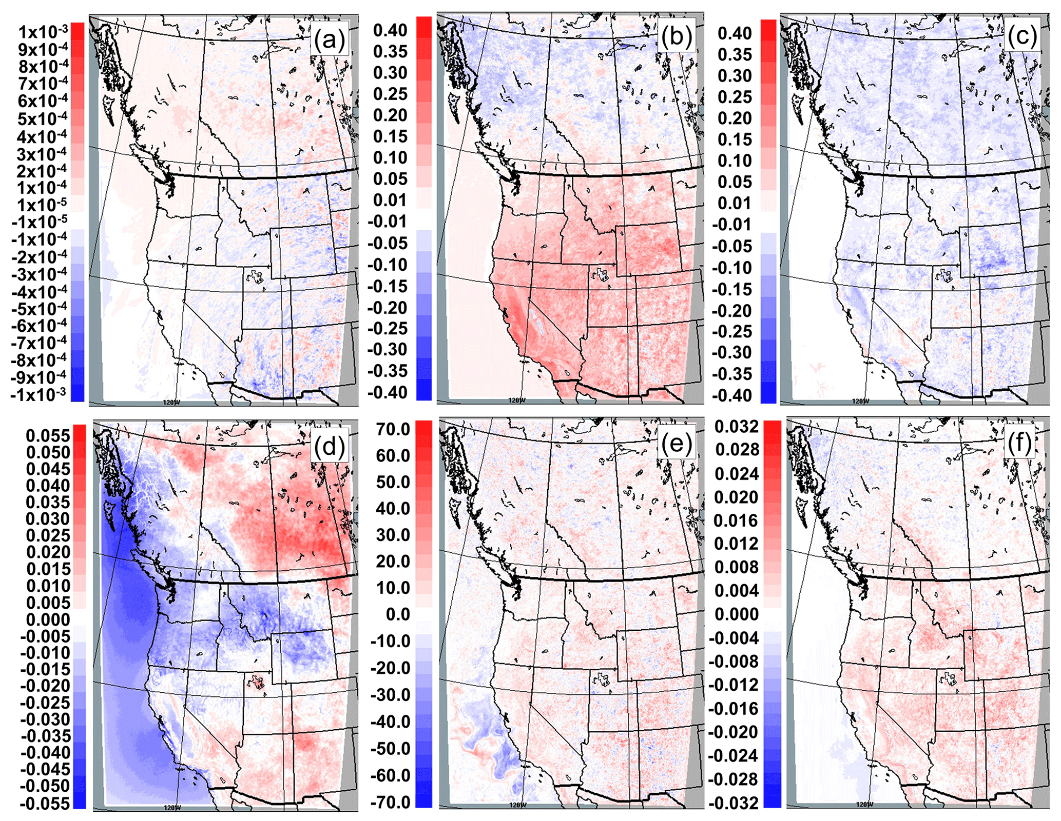
Figure 18Differences in average meteorological fields (feedback–no-feedback; red values indicate more positive values in the feedback simulation than in the no-feedback simulation). Panels show average difference in (a) specific humidity (g kg⁻¹); (b) air temperature (^∘C), (c) dew-point temperature (^∘C), (d) surface pressure (mb), (e) planetary boundary layer height (m), and (f) friction velocity (m s⁻¹).

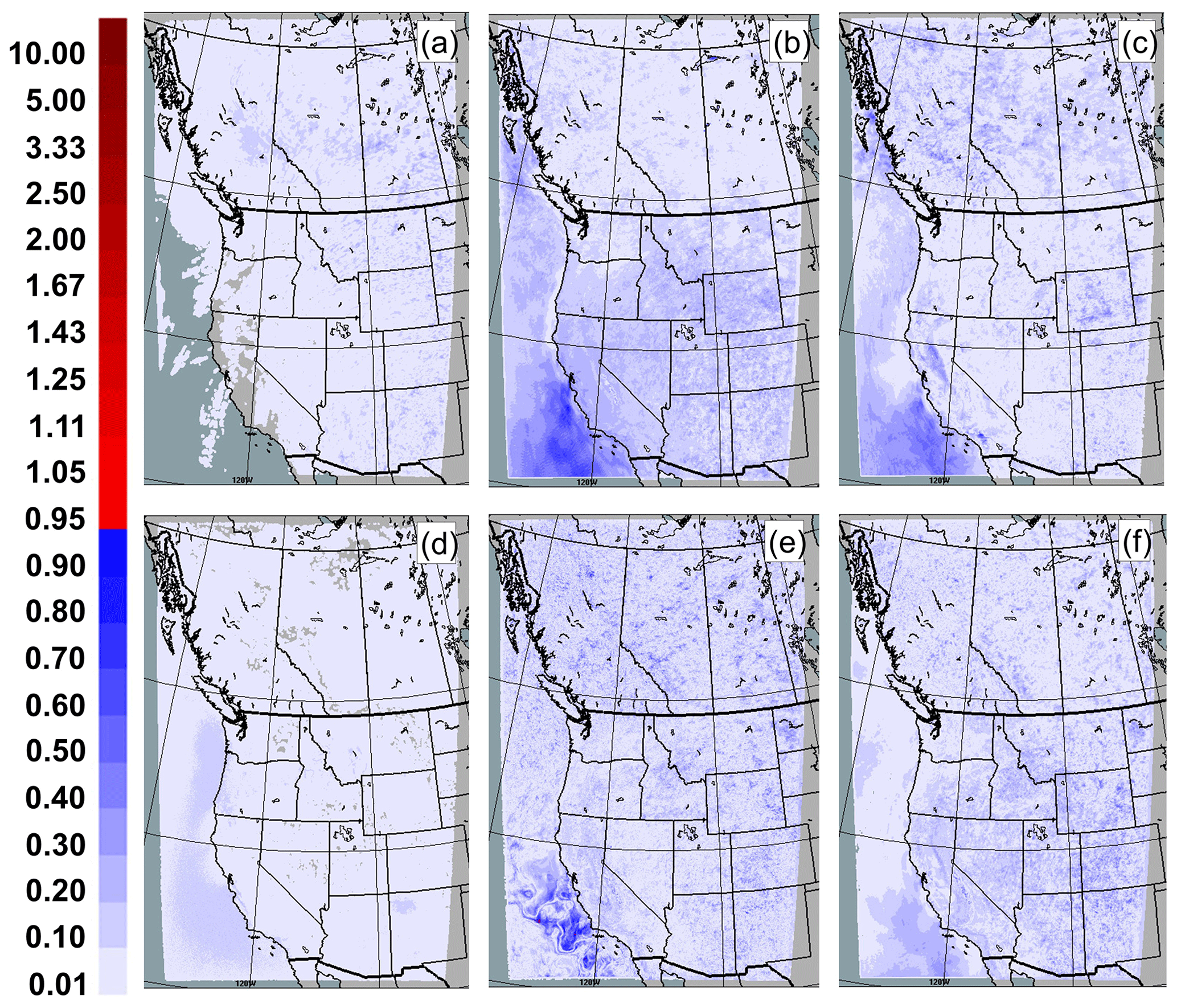
Figure 1990 % confidence ratios, with the same fields as Fig. 18. Values greater than 1 indicate significantly different results at or greater than the 90 % confidence level.

Figure 20(a, b) Difference in mean (feedback–no-feedback) temperature simulations along south–north and east–west cross sections through the middle of the model domain. (c, d) Corresponding confidence ratio of mean temperature differences – red areas indicate ratio values greater than unity, i.e., significance at or above the 90 % confidence level.

Download

Several systematic changes in the average values of the model's meteorological output fields were noted due to the use of feedbacks relative to aerosol property climatologies (Fig. 18), although all fall below the 90 % confidence level for the difference in the mean values between the two simulations (Fig. 19). Specific humidity increased in the region most affected by fires (Fig. 18a), and surface air temperature decreased below the smoke plumes while increasing further south (Fig. 18b), while dew-point temperature decreased (Fig. 18c), implying a decrease in relative humidity with feedbacks. Surface pressure increased over the land (mostly east of the Rockies), particularly in the region downwind of the Alberta–Saskatchewan fires while decreasing over the ocean (Fig. 18d). Planetary boundary layer height increased over the land (Fig. 18e) except in the immediate vicinity of the Alberta–Saskatchewan fires, consistent with decreased atmospheric stability in the lowest part of the atmosphere. The friction velocity also increased with the use of feedbacks (Fig. 18f); this is consistent with a decrease in stability and an increase in turbulent energy. The air temperature increases occur at the surface south of the forest-fire-impacted region and above roughly 750 mb, decreasing temperatures from the surface in the forest-fire-impacted region up to 750 mb (Fig. 20a and b). Feedbacks thus increase near-surface temperatures, relative to the no-feedback meteorological model's simple aerosol climatology, in regions far from the fires, decreasing them near the fires, decrease temperatures in the lower free troposphere, and increase temperatures further aloft. All of these differences between feedback and no-feedback simulations, despite their large geographic range, fall below the local 90 % confidence ratio. However, when the differences in air temperature associated with feedback and no-feedback forecasts are compared to observations across the entire domain (as opposed to at grid point locations as in Figs. 18 and 19), the 90 % confidence level is exceeded, both at the surface at specific forecast times (Fig. 6a), and at multiple heights aloft at the 12th and 24th forecast hours (Figs. 12 and 13).

4.2 Effects of feedbacks on time-averaged chemistry

In the previous meteorological impacts section, changes in aerosol loading relative to the climatology, dominated by forest fires, were shown to have a significant impact on cloud formation and atmospheric temperatures through ADE and AIE. These might be expected to in turn influence and be influenced by particulate matter emitted by the forest fires, with the plume rise of the forest fires dependent on the meteorological changes. Air temperatures increase slightly in the model surface layer south of the fires (Fig. 18b, +0.01 to +0.05 ^∘C) but decrease at greater magnitudes through the rest of the lower troposphere (surface near the fires to hybrid level 0.749, Fig. 20a), with a maximum decrease of −0.5 ^∘C between hybrid levels 0.893 and 0.848. The reduction in temperatures between hybrid levels 0.90 to 0.70 from the impact of the smoke plumes is similar to the findings of Saponaro et al. (2017). These changes in air temperature imply a decrease in near-surface atmospheric stability associated with feedbacks, given that the overall temperature gradient from the surface has become more negative (that is, the ambient lapse rate has increased). Rising air parcels will follow an adiabatic lapse rate; these increases in the ambient lapse rate imply that rising air parcels will have an increasing tendency to be warmer than their environment. Feedbacks have thus reduced atmospheric stability within the forest-fire smoke in the lowest part of the atmosphere; the atmosphere there has become more unstable. Meanwhile, the feedbacks decrease the environmental lapse rate further aloft above the forest-fire smoke, between hybrid levels 0.848 and 0.339. Rising air parcels in this region following an adiabatic lapse rate will thus have an increasing tendency to be colder than their environment – the atmosphere above the smoke plumes has become more stable. This is echoed by the response of the concentration fields to the near-surface stability change, as can be seen through comparisons of the PM_2.5, NO₂, and O₃ surface concentration changes (Fig. 21) and the vertical cross sections (Figs. 22–24), respectively.

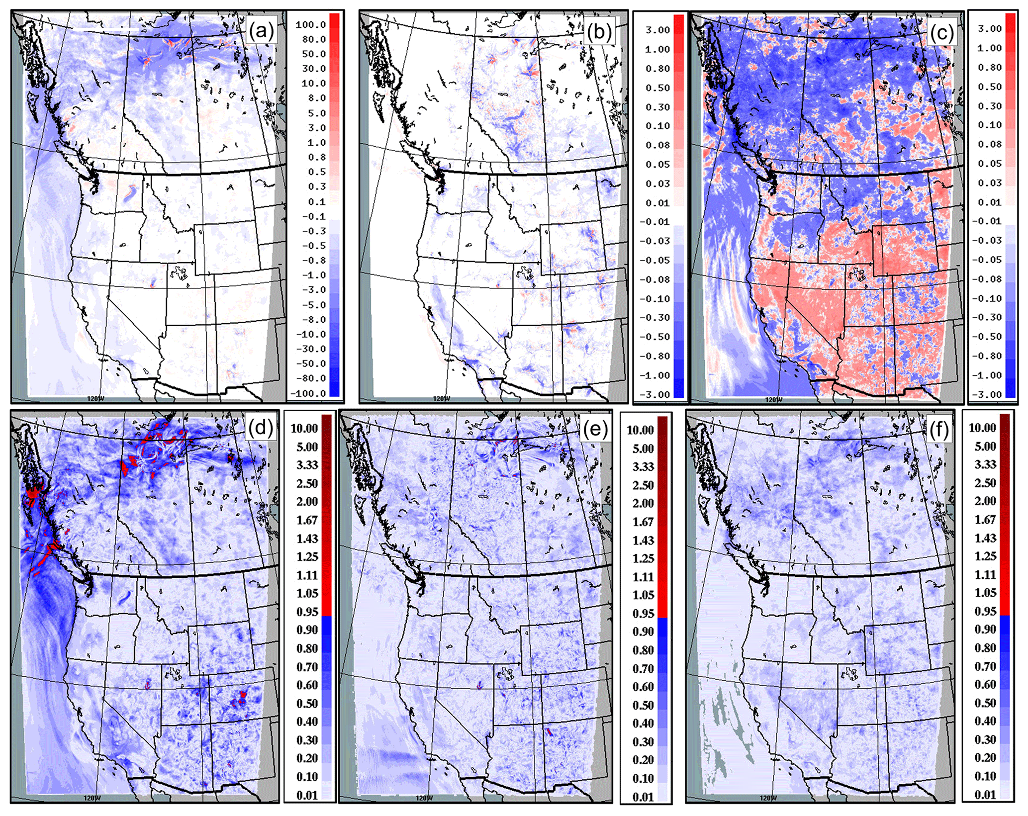
Figure 21(a–c) Difference (feedback–no-feedback) in surface mean PM_2.5 (µg m⁻³), NO₂ (ppbv), and O₃ (ppbv), respectively. (d–f) Corresponding confidence ratio of mean differences – red areas indicate ratio values greater than unity, i.e., significance at or above the 90 % confidence level.

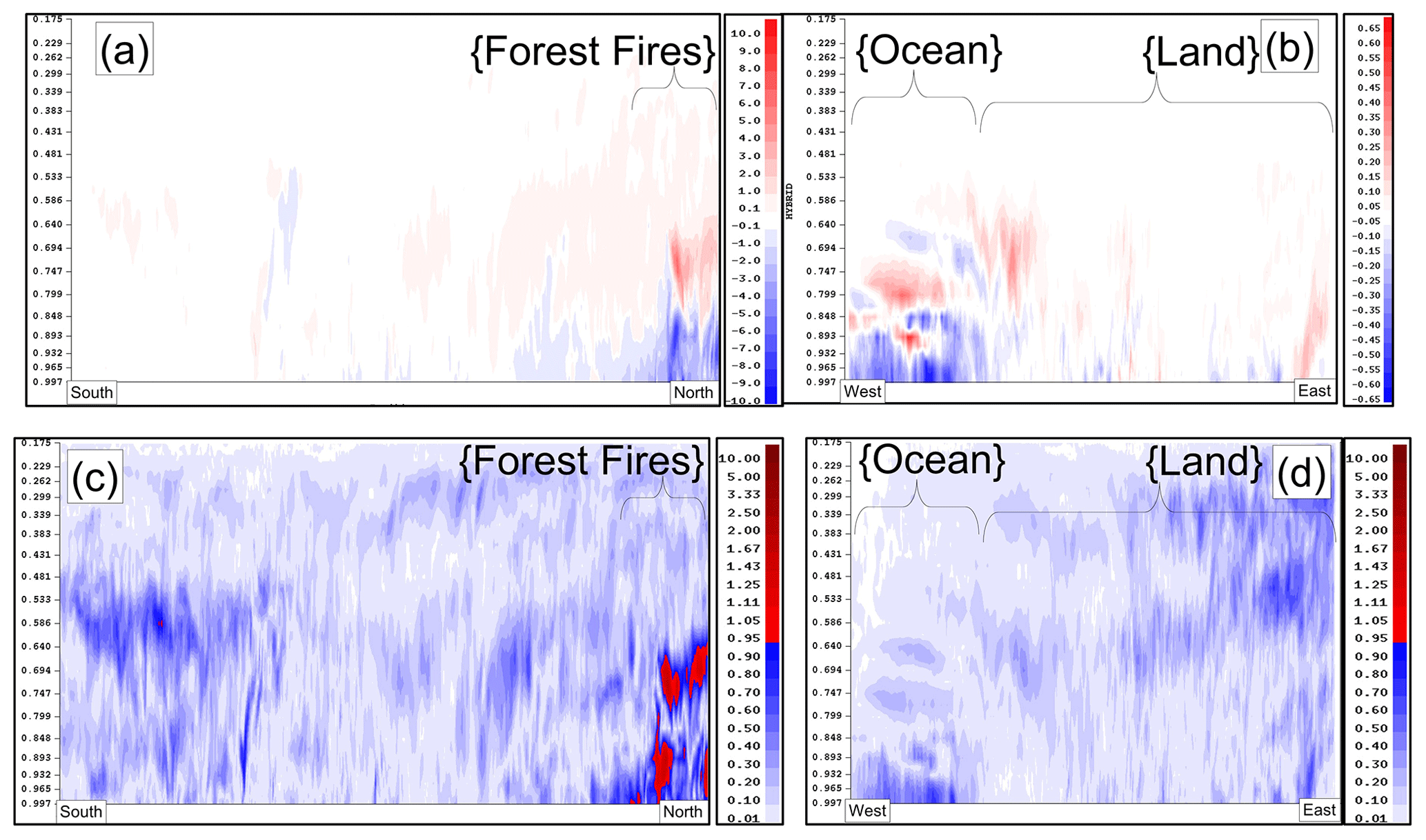
Figure 22(a, b) Difference (feedback–no-feedback) in predicted mean PM_2.5 (µg m⁻³), along domain-center south–north and west–east cross sections. (c, d) Corresponding confidence ratio of mean differences – red areas indicate ratio values greater than unity, i.e., significance at or above the 90 % confidence level. Note that colour bar scales differ between (a) and (b).

Download

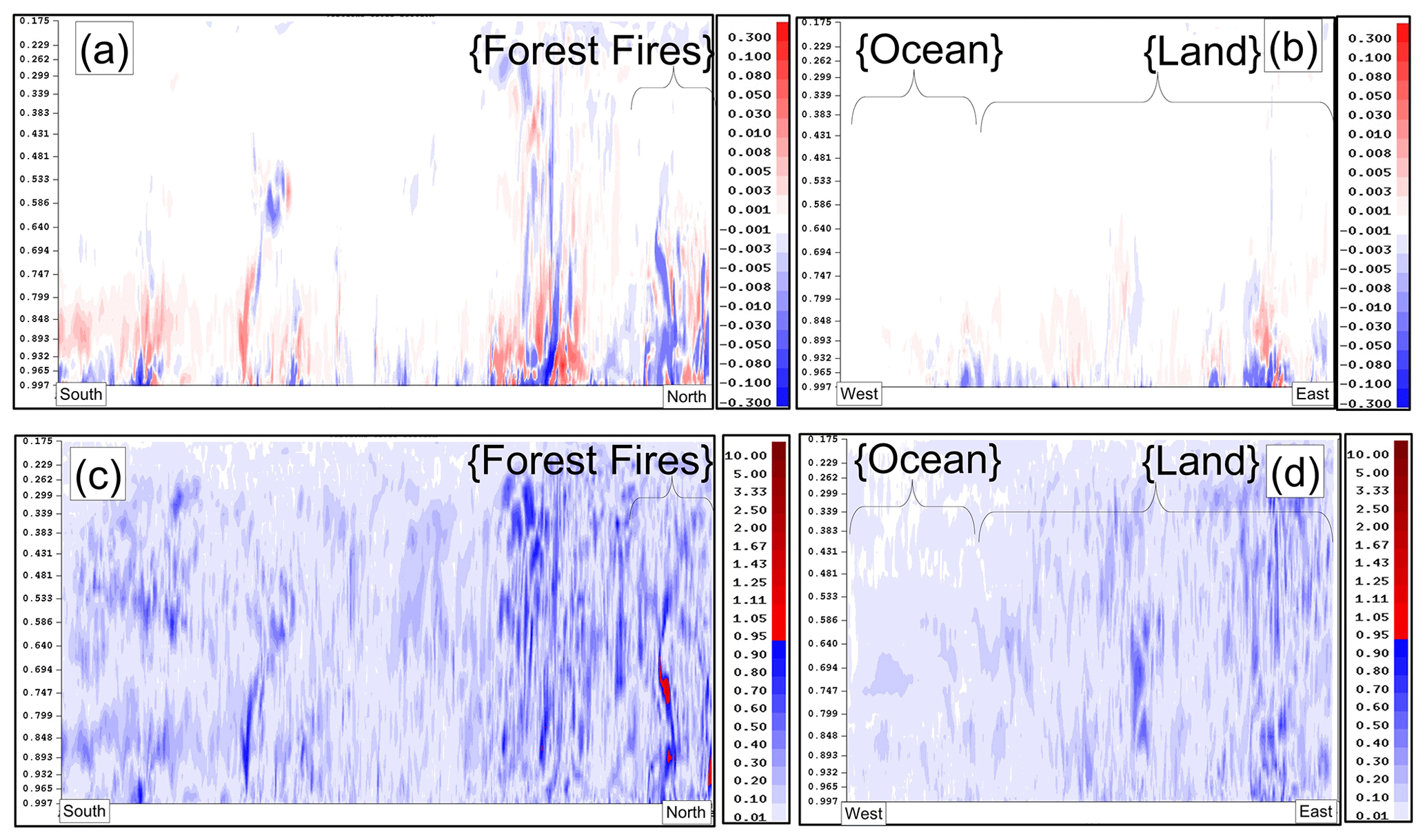
Figure 23(a, b) Difference (feedback–no-feedback) in predicted mean NO₂ (ppbv), along domain-center south–north and west–east cross sections. (c, d) Corresponding confidence ratio of mean differences – red areas indicate ratio values greater than unity, i.e., significance at or above the 90 % confidence level.

Download

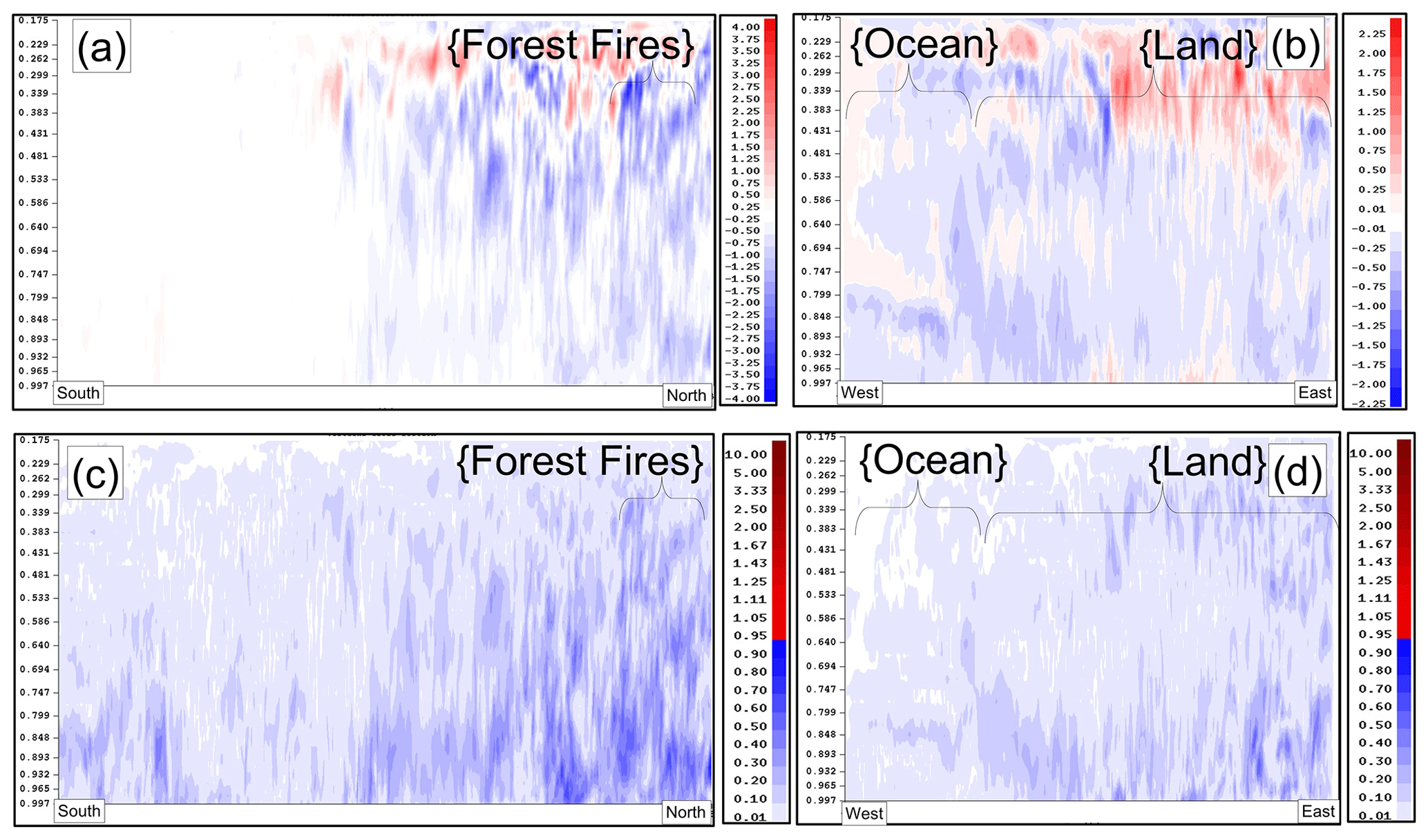
Figure 24(a, b) Difference (feedback–no-feedback) in predicted mean O₃ (ppbv), along domain-center south–north and west–east cross sections. (c, d) Corresponding confidence ratio of mean differences – red areas indicate ratio values greater than unity, i.e., significance at or above the 90 % confidence level. Note that colour bar scales differ between (a) and (b).

Download

Changes above the 90 % confidence level for PM_2.5 and NO₂ occur near the forest fires themselves (red regions, near top of model domain; Fig. 21a and b), though they remain below 90 % confidence for O₃ (Fig. 21c).

Feedbacks result in near-surface PM_2.5 decreases in the regions downwind of the forest fires (Figs. 21a and 22a; note the large blue region and more intense blue region near surface in Fig. 22a), suggesting less PM_2.5 mass is present near the surface due to the feedbacks. Given the increase in near-surface stability below the fire plumes noted above, this change in the vertical distribution probably reflects a decrease in downward diffusive mixing of the forest-fire plumes once aloft – the feedbacks thus have a tendency to increase the smoke plume concentrations aloft, by preventing the downward mixing of smoke injected by the fires. These PM_2.5 concentration effects rise above the 90 % confidence level within the region closest to the fires.

Feedbacks result in an increase in near-surface NO₂ in several inland urban centers and less NO₂ at surface level downwind (Fig. 21b; though these differences are only significant at the 90 % confidence level within the forest-fire plumes (Figs. 21e and 23c). Ocean versus land NO₂ differences remain below the 90 % confidence level.

Feedbacks decreased lower troposphere O₃ near the forest fires (Figs. 21c and 24a), while increasing O₃ near and above hybrid level 0.383. The forest fires are also the only area where the differences between mean ozone forecasts approach 90 % confidence.

Overall, the most significant effects of the feedbacks were (1) increases in PM_2.5 aloft and decreases near the surface in areas impacted by the fires; (2) increases in NO₂ aloft and decreases near the surface near the fires, to a lesser extent than PM_2.5; and (3) decreases in lower troposphere O₃, particularly near the surface in the region impacted by the fires.

The feedback-induced changes in primary and secondary pollutants in the forest-fire regions are consistent with the decrease in atmospheric stability noted above – a greater proportion of the primary particulate matter and NO₂ resulting from near-surface forest-fire emissions of NO remain aloft with the addition of feedbacks. The decrease in surface ozone and increase further aloft in the fire region (Fig. 24a) spatially match the decrease in surface NO₂ (Fig. 22a). Chemically, this may imply that the changes associated with feedbacks occur in NO_x-limited environments, i.e., with relatively high $\mathrm{VOC}/{\mathrm{NO}}_x$ ratios, since in these environments, decreases in NO_x emissions may lead to decreases in the rate of secondary O₃ formation. Alternatively, the reduction in near-surface O₃ concentrations may reflect a decrease in light levels reaching the surface due to cloud attenuation (aerosol indirect effect), with the resultant lower photolysis rates resulting in a reduction in surface photochemical ozone production.

Our analysis thus suggests that a net enhanced upward transport occurs in forest-fire plumes due to feedbacks and that this transport is linked to the following feedback-induced changes:

• 1.

  increases in local near-surface atmospheric stability, reducing downward mixing of particulate plumes once aloft (Fig. 22a);

• 2.

  increases in cloud droplet numbers throughout the lower troposphere (Fig. 15a); and

• 3.

  increases in raindrop numbers aloft (Fig. 16a).

This combination suggests the presence of an AIE feedback loop – increased lower atmosphere stability results in a greater proportion of particulate matter remaining aloft, in turn resulting in more particles remaining at higher levels in the atmosphere where they may act as cloud condensation nuclei, increasing cloud droplets aloft (Fig. 15a). This in turn results in increased lower middle troposphere cooling, through the first AIE (increase in cloud droplet numbers aloft, leading to increased cloud albedo and cooling of the atmosphere below the cloud tops), while the corresponding decreases in particles and cloud condensation nuclei at lower levels result in a smaller near-surface impact on the AIE and ADE, hence relatively minor changes in near-surface temperatures (Fig. 20a). This combination maintains a feedback-induced near-surface unstable temperature gradient, relative to the no-feedback simulation employing aerosol property climatologies. We acknowledge that these changes in temperature fall below the 90 % confidence level for the averages over all times, though note that differences in mean bias relative to observations for the two simulations became significantly different at specific times of day in the forecasts (Fig. 6a; hours 3, 6, 15, and 18, corresponding to 15:00, 18:00, 03:00, and 06:00 UT or 09:00, 12:00, 21:00, and 00:00 MDT), implying that the temperature changes at these specific times reach a higher level of significance. Similarly, Figs. 12 and 13 show reductions in the near-surface temperature biases with the use of feedbacks.

4.3 Summary: differences in forecast simulation-period averages

Relative to the no-feedback simulation employing an aerosol climatology, the AIE feedback as simulated here is associated with increases in near-surface stability over both ocean- and forest-fire-influenced land areas. Over oceans, near-surface particulate matter is removed as cloud condensation nuclei, resulting in increased cloud droplet numbers, maintaining the temperature gradient through the first aerosol indirect effect. In the vicinity of forest fires, increases in near-surface stability result in more PM_2.5 remaining aloft, increasing the availability of cloud condensation nuclei aloft, increasing cloud droplet numbers aloft, hence also maintaining the less stable near-surface temperature gradient through the first aerosol indirect effect. We note that the ADE may also play a weak role, particularly in the southern part of the domain, where lower atmosphere temperature gradient increases are not accompanied by significant changes in cloud droplet numbers (Fig. 15a, southern half of the cross section) but are accompanied by significant though small magnitude increases in PM_2.5 in the lower atmosphere (Fig. 22a, southern half of cross section) and temperature profile changes (Fig. 20) below the 90 % confidence level.