
Prediction of protein function using a deep convolutional neural network ensemble
- Published
- Accepted
- Received
- Academic Editor
- James Procter
- Subject Areas
- Bioinformatics, Computational Biology, Data Mining and Machine Learning
- Keywords
- Enzyme classification, Function predition, Deep learning, Convolutional neural networks, Structure representation
- Copyright
- © 2017 Zacharaki
- Licence
- This is an open access article distributed under the terms of the Creative Commons Attribution License, which permits unrestricted use, distribution, reproduction and adaptation in any medium and for any purpose provided that it is properly attributed. For attribution, the original author(s), title, publication source (PeerJ Computer Science) and either DOI or URL of the article must be cited.
- Cite this article
- 2017. Prediction of protein function using a deep convolutional neural network ensemble. PeerJ Computer Science 3:e124 https://doi.org/10.7717/peerj-cs.124
Abstract
Background
The availability of large databases containing high resolution three-dimensional (3D) models of proteins in conjunction with functional annotation allows the exploitation of advanced supervised machine learning techniques for automatic protein function prediction.
Methods
In this work, novel shape features are extracted representing protein structure in the form of local (per amino acid) distribution of angles and amino acid distances, respectively. Each of the multi-channel feature maps is introduced into a deep convolutional neural network (CNN) for function prediction and the outputs are fused through support vector machines or a correlation-based k-nearest neighbor classifier. Two different architectures are investigated employing either one CNN per multi-channel feature set, or one CNN per image channel.
Results
Cross validation experiments on single-functional enzymes (n = 44,661) from the PDB database achieved 90.1% correct classification, demonstrating an improvement over previous results on the same dataset when sequence similarity was not considered.
Discussion
The automatic prediction of protein function can provide quick annotations on extensive datasets opening the path for relevant applications, such as pharmacological target identification. The proposed method shows promise for structure-based protein function prediction, but sufficient data may not yet be available to properly assess the method’s performance on non-homologous proteins and thus reduce the confounding factor of evolutionary relationships.
Introduction
Metagenomics has led to a huge increase of protein databases and the discovery of new protein families (Godzik, 2011). While the number of newly discovered, but possibly redundant, protein sequences rapidly increases, experimentally verified functional annotation of whole genomes remains limited. Protein structure, i.e., the 3D configuration of the chain of amino acids, is a very good predictor of protein function, and in fact a more reliable predictor than protein sequence because it is far more conserved in nature (Illergård, Ardell & Elofsson, 2009).
By now, the number of proteins with functional annotation and experimentally predicted structure of their native state (e.g., by NMR spectroscopy or X-ray crystallography) is adequately large to allow machine learning models to be trained that will be able to perform automatic functional annotation of unannotated proteins (Amidi et al., 2017). Also, as the number of protein sequences rapidly grows, the overwhelming majority of proteins can only be annotated computationally. In this work enzymatic structures from the Protein Data Bank (PDB) are considered and the enzyme commission (EC) number is used as a fairly complete framework for annotation. The EC number is a numerical classification scheme based on the chemical reactions the enzymes catalyze, proven by experimental evidence (Webb, 1992).
There have been plenty machine learning approaches in the literature for automatic enzyme annotation. A systematic review on the utility and inference of various computational methods for functional characterization is presented in Sharma & Garg (2014), while a comparison of machine learning approaches can be found in Yadav & Tiwari (2015). Most methods use features derived from the amino acid sequence and apply support vector machines (SVM) (Cai et al., 2003; Han et al., 2004; Dobson & Doig, 2005; Chen et al., 2006; Zhou et al., 2007; Lu et al., 2007; Lee et al., 2009; Qiu et al., 2010; Wang et al., 2010; Wang et al., 2011; Amidi et al., 2016), k-nearest neighbor (kNN) classifier (Huang et al., 2007; Shen & Chou, 2007; Nasibov & Kandemir-Cavas, 2009), classification trees/forests (Lee et al., 2009; Kumar & Choudhary, 2012; Nagao, Nagano & Mizuguchi, 2014; Yadav & Tiwari, 2015), and neural networks (Volpato, Adelfio & Pollastri, 2013). In Borgwardt et al. (2005) sequential, structural and chemical information was combined into one graph model of proteins which was further classified by SVM. However, there has been little work in the literature on automatic enzyme annotation based only on structural information. A Bayesian approach (Borro et al., 2006) for enzyme classification using structure derived properties achieved 45% accuracy. Amidi et al. (2016) obtained 73.5% classification accuracy on 39,251 proteins from the PDB database when they used only structural information.
In the past few years, deep learning techniques, and particularly convolutional neural networks, have rapidly become the tool of choice for tackling many challenging computer vision tasks, such as image classification (Krizhevsky, Sutskever & Hinton, 2012). The main advantage of deep learning techniques is the automatic exploitation of features and tuning of performance in a seamless fashion, that simplifies the conventional image analysis pipelines. CNNs have recently been used for protein secondary structure prediction (Spencer, Eickholt & Cheng, 2015; Li & Shibuya, 2015). In Spencer, Eickholt & Cheng (2015) prediction was based on the position-specific scoring matrix profile (generated by PSI-BLAST), whereas in Li & Shibuya (2015) 1D convolution was applied on features related to the amino acid sequence. Also, a deep CNN architecture was proposed in Lin, Lanchantin & Qi (2016) to predict protein properties. This architecture used a multilayer shift-and-stitch technique to generate fully dense per-position predictions on protein sequences. To the best of the author’s knowledge, deep CNNs have not been used for prediction of protein function so far.
In this work the author exploits experimentally acquired structural information of enzymes and apply deep learning techniques in order to produce models that predict enzymatic function based on structure. Novel geometric descriptors are introduced and the efficacy of the approach is illustrated by classifying a dataset of 44,661 enzymes from the PDB database into the l = 6 primary categories: oxidoreductases (EC1), transferases (EC2), hydrolases (EC3), lyases (EC4), isomerases (EC5), ligases (EC6). The novelty of the proposed method lies first in the representation of the 3D structure as a “bag of atoms (amino acids)” which are characterized by geometric properties, and secondly in the exploitation of the extracted feature maps by deep CNNs. Although assessed for enzymatic function prediction, the method is not based on enzyme-specific properties and therefore can be applied (after re-training) for automatic large-scale annotation of other 3D molecular structures, thus providing a useful tool for data-driven analysis. In the following sections more details on the implemented framework are first provided, including the representation of protein structure, the CNN architecture and the fusion process of the network outputs. Then the evaluation framework and the obtained results are presented, followed by some discussion and conclusions.
Methods
Data-driven CNN models tend to be domain agnostic and attempt to learn additional feature bases that cannot be represented through any handcrafted features. It is hypothesized that by combining “amino acid specific” descriptors with the recent advances in deep learning we can boost model performance. The main advantage of the proposed method is that it exploits complementarity in both data representation phase and learning phase. Regarding the former, the method uses an enriched geometric descriptor that combines local shape features with features characterizing the interaction of amino acids on this 3D spatial model. Shape representation is encoded by the local (per amino acid type) distribution of torsion angles (Bermejo, Clore & Schwieters, 2012). Amino acid interactions are encoded by the distribution of pairwise amino acid distances. While the torsion angles and distance maps are usually calculated and plotted for the whole protein (Bermejo, Clore & Schwieters, 2012), in the current approach they are extracted for each amino acid type separately, therefore characterizing local interactions. Thus, the protein structure is represented as a set of multi-channel images which can be introduced into any machine learning scheme designed for fusing multiple 2D feature maps. Moreover, it should be noted that the utilized geometric descriptors are invariant to global translation and rotation of the protein, therefore previous protein alignment is not required.
Our method constructs an ensemble of deep CNN models that are complementary to each other. The deep network outputs are combined and introduced into a correlation-based kNN classifier for function prediction. For comparison purposes, support vector machines were also implemented for final classification. Two system architectures are investigated in which the multiple image channels are considered jointly or independently, as will be described next. Both architectures use the same CNN structure (within the highlighted boxes) which is illustrated in Fig. 1.
Figure 1: The deep CNN ensemble for protein classification.
In this framework (Architecture 1) each multi-channel feature set is introduced to a CNN and results are combined by kNN or SVM classification. The network includes layers performing convolution (Conv), batch normalization (Bnorm), rectified linear unit (ReLU) activation, dropout (optionally) and max-pooling (Pool). Details are provided in ‘Classification by deep CNNs’.
Representation of protein structure
The building blocks of proteins are amino acids which are linked together by peptide bonds into a chain. The polypeptide folds into a specific conformation depending on the interactions between its amino acid side chains which have different chemistries. Many conformations of this chain are possible due to the rotation of the chain about each carbon (Cα) atom. For structure representation, two sets of feature maps were used. They express the shape of the protein backbone and the distances between the protein building blocks (amino acids). The use of global rotation and translation invariant features is preferred over features based on the Cartesian coordinates of atoms, in order to avoid prior protein alignment, which is a bottleneck in the case of large datasets with proteins of several classes (unknown reference template space). The feature maps were extracted for every amino acid being present in the dataset including the 20 standard amino acids, as well as asparagine/aspartic (ASX), glutamine/glutamic (GLX), and all amino acids with unidentified/unknown residues (UNK), resulting in m = 23 amino acids in total.
Torsion angles density
The shape of the protein backbone was expressed by the two torsion angles of the polypeptide chain which describe the rotations of the polypeptide backbone around the bonds between N-Cα (angle ϕ) and Cα-C (angle ψ). All amino acids in the protein were grouped according to their type and the density of the torsion angles ϕ and ψ(∈[ − 180, 180]) was estimated for each amino acid type based on the 2D sample histogram of the angles (also known as Ramachandran diagram) using equally sized bins (number of bins hA = 19). The histograms were not normalized by the number of instances, therefore their values indicate the frequency of each amino acid within the polypeptide chain. In the obtained feature maps (XA), with dimensionality [hA × hA × m], the number of amino acids (m) corresponds to the number of channels. Smoothness in the density function was achieved by moving average filtering, i.e., by convoluting the density map with a 2D Gaussian kernel (σ = 0.5).
Density of amino acid distances
For each amino acid ai, i = 1, …, m, distances to amino acid aj, j = 1, …, m, in the protein are calculated based on the coordinates of the Cα atoms for the residues and stored as an array dij. Since the size of the proteins varies significantly, the length of the array dij is different across proteins, thus not directly comparable. In order to standardize measurements, the sample histogram of dij is extracted (using equally sized bins) and smoothed by convolution with a 1D Gaussian kernel (σ = 0.5). The processing of all pairs of amino acids resulted in feature maps (XD) of dimension [m × m × hD], where hD = 8 is the number of histogram bins (considered as number of channels in this case).
Classification by deep CNNs
Feature extraction stage of each CNN
The CNN architecture employs three computational blocks of consecutive convolutional, batch normalization, rectified linear unit (ReLU) activation, dropout (optionally) and max-pooling layers, and a fully-connected layer. The convolutional layer computes the output of neurons that are connected to local regions in the input in order to extract local features. It applies a 2D convolution between each of the input channels and a set of filters. The 2D activation maps are calculated by summing the results over all channels and then stacking the output of each filter to produce the output 3D volume. Batch normalization normalizes each channel of the feature map by averaging over spatial locations and batch instances. The ReLU layer applies an element-wise activation function, such as the max(0, x) thresholding at zero. The dropout layer is used to randomly drop units from the CNN during training to reduce overfitting. Dropout was used only for the XA feature set. The pooling layer performs a downsampling operation along the spatial dimensions in order to capture the most relevant global features with fixed length. The max operator was applied within a [2 × 2] neighborhood. The last layer is fully-connected and represents the class scores.
Training and testing stage of each CNN
The output of each CNN is a vector of probabilities, one for each of the l possible enzymatic classes. The CNN performance can be measured by a loss function which assigns a penalty to classification errors. The CNN parameters are learned to minimize this loss averaged over the annotated (training) samples. The softmax loss function (i.e., the softmax operator followed by the logistic loss) is applied to predict the probability distribution over categories. Optimization was based on an implementation of stochastic gradient descent. At the testing stage, the network outputs after softmax normalization are used as class probabilities.
Fusion of CNN outputs using two different architectures
Two fusion strategies were implemented. In the first strategy (Architecture 1) the two feature sets, XA and XD, are each introduced into a CNN, which performs convolution at all channels, and then the l class probabilities produced for each feature set are combined into a feature vector of length l∗2. In the second strategy (Architecture 2), each one of the (m = 23 or hD = 8) channels of each feature set is introduced independently into a CNN and the obtained class probabilities are concatenated into a vector of l∗m features for XA and l∗hD features for XD, respectively. These two feature vectors are further combined into a single vector of length l∗(m + hD) (=186). For both architectures, kNN classification was applied for final class prediction using as distance measure between two feature vectors, x1 and x2, the metric 1 − cor(x1, x2), where cor is the sample Spearman’s rank correlation. The value k = 12 was selected for all experiments. For comparison, fusion was also performed with linear SVM classification (Chang & Lin, 2011). The code was developed in MATLAB environment and the implementation of CNNs was based on MatConvNet (Vedaldi & Lenc, 2015).
Results
The protein structures (n = 44, 661) were collected from the PDB. Only enzymes that occur in a single class were processed, whereas enzymes that perform multiple reactions and are hence associated with multiple enzymatic functions were excluded. Since protein sequence was not examined during feature extraction, all enzymes were considered without other exclusion criteria, such as small sequence length or homology bias. The dataset was unbalanced in respect to the different classes. The number of samples per class is shown in Table 1. The dataset was split into five folds. Four folds were used for training and one for testing. The training samples were used to learn the parameters of the network (such as the weights of the convolution filters), as well as the parameters of the subsequent classifiers used during fusion (SVM or kNN model). Once the network was trained, the class probabilities were obtained for the testing samples, which were introduced into the trained SVM or kNN classifier for final prediction. The SVM model was linear and thus didn’t require any hyper-parameter optimization. Due to the lack of hyper-parameters, no extra validation set was necessary. On the side, the author also examined non-linear SVM with a Gaussian radial basis function kernel, but didn’t observe any significant improvement; thus, the corresponding results are not reported.
| Architecture 1 | Architecture 2 | ||||
|---|---|---|---|---|---|
| Class | Samples | Linear-SVM | kNN | Linear-SVM | kNN |
| EC1 | 8,075 | 86.4 | 88.8 | 91.2 | 90.6 |
| EC2 | 12,739 | 84.0 | 87.5 | 88.0 | 91.7 |
| EC3 | 17,024 | 88.7 | 91.3 | 89.6 | 94.0 |
| EC4 | 3,114 | 79.4 | 78.4 | 84.9 | 80.7 |
| EC5 | 1,905 | 69.5 | 68.6 | 79.6 | 77.0 |
| EC6 | 1,804 | 61.0 | 60.6 | 73.6 | 70.4 |
| Total | 44,661 | 84.4 | 86.7 | 88.0 | 90.1 |
A classification result was deemed a true positive if the match with the highest probability was in first place in a rank-ordered list. The classification accuracy (percentage of correctly classified samples over all samples) was calculated for each fold and then averaged across the five folds.
Classification performance
Common options for the network were used, except of the size of the filters which was adjusted to the dimensionality of the input data. Specifically, the convolutional layer used neurons with a receptive field of size 5 for the first two layers and 2 for the third layer. The stride (specifying the sliding of the filter) was always 1. The number of filters was 20, 50 and 500 for the three layers, respectively, and the learning rate was 0.001. The batch size was selected according to the information amount (dimensionality) of the input. It was assumed (and verified experimentally) that for more complicated data, a larger number of samples is required for learning. One thousand samples per batch were used for Architecture 1, which takes as input all channels, and 100 samples per batch for Architecture 2, in which an independent CNN is trained for each channel. The dropout rate was 20%. The number of epochs was adjusted to the rate of convergence for each architecture (300 for Architecture 1 and 150 for Architecture 2).
The average classification accuracy over the five folds for each enzymatic class is shown in Table 1 for both fusion schemes, whereas the analytic distribution of samples in each class is shown in the form of confusion matrices in Table 2.
| Classifier | Prediction by Architecture 1 | Prediction by Architecture 2 | |||||||||||
|---|---|---|---|---|---|---|---|---|---|---|---|---|---|
| 1 | 2 | 3 | 4 | 5 | 6 | 1 | 2 | 3 | 4 | 5 | 6 | ||
| Linear-SVM | EC1 | 86.5 | 4.9 | 4.8 | 1.8 | 1.1 | 1.0 | 91.2 | 2.9 | 1.9 | 2.2 | 1.1 | 0.7 |
| EC2 | 3.4 | 84.0 | 7.9 | 1.9 | 1.2 | 1.6 | 3.6 | 88.0 | 3.5 | 2.2 | 1.2 | 1.5 | |
| EC3 | 2.4 | 6.1 | 88.7 | 1.0 | 0.8 | 1.0 | 2.3 | 4.1 | 89.6 | 1.6 | 1.2 | 1.2 | |
| EC4 | 4.4 | 7.3 | 5.7 | 79.4 | 1.8 | 1.3 | 4.3 | 4.9 | 2.7 | 84.9 | 1.7 | 1.4 | |
| EC5 | 7.0 | 10.1 | 9.0 | 2.9 | 69.4 | 1.6 | 4.5 | 5.4 | 4.7 | 4.4 | 79.5 | 1.7 | |
| EC6 | 5.9 | 15.5 | 13.0 | 2.3 | 2.3 | 61.0 | 5.5 | 10.3 | 5.4 | 3.3 | 1.9 | 73.6 | |
| kNN | EC1 | 88.8 | 5.0 | 4.5 | 0.7 | 0.5 | 0.5 | 90.6 | 4.4 | 4.6 | 0.3 | 0.1 | 0.0 |
| EC2 | 2.5 | 87.5 | 7.4 | 1.0 | 0.6 | 1.1 | 1.7 | 91.7 | 5.8 | 0.3 | 0.2 | 0.4 | |
| EC3 | 1.8 | 5.4 | 91.3 | 0.5 | 0.4 | 0.6 | 1.2 | 4.4 | 94.0 | 0.2 | 0.1 | 0.2 | |
| EC4 | 3.8 | 9.1 | 7.2 | 78.5 | 1.1 | 0.4 | 3.7 | 8.4 | 6.9 | 80.7 | 0.1 | 0.1 | |
| EC5 | 6.1 | 11.5 | 10.7 | 2.3 | 68.5 | 1.0 | 3.5 | 9.7 | 8.6 | 0.9 | 76.9 | 0.3 | |
| EC6 | 4.9 | 18.8 | 13.5 | 1.0 | 1.3 | 60.6 | 4.2 | 14.1 | 10.3 | 0.7 | 0.3 | 70.5 | |
In order to further assess the performance of the deep networks, receiver operating characteristic (ROC) curves and area-under-the-curve (AUC) values were calculated for each class for the selected scheme (based on kNN and Architecture 2), as shown in Fig. 2). The calculations were performed based on the final decision scores in a one-versus-rest classification scheme. The decision scores for the kNN classifier reflected the ratio of the within-class neighbors over total number of neighbors. The ROC curve represents the true positive rate against the false positive rate and was produced by averaging over the five folds of the cross-validation experiments.
Figure 2: ROC curves for each enzymatic class based on kNN and Architecture 2.
(A) EC1, (B) EC2, (C) EC3, (D) EC4, (E) EC5, (F) EC6.
Effect of sequence redundancy and sample size
Analysis of protein datasets is often performed after removal of redundancy, such that the remaining entries do not overreach a pre-arranged threshold of sequence identity. In the previously presented results, sequence/threshold metrics were not applied to remove sequence-redundancy. Although structure similarity is affected by sequence similarity, the aim was not to lose structural entries (necessary for efficient learning) over a sequence based threshold cutoff. Also, only X-ray crystallography data were used; such data represent a ‘snapshot’ of a given protein’s 3D structure. In order not to miss the multiple poses that the same protein may adopt in different crystallography experiments, the whole dataset was explored.
Subsequently, the performance of the method was also investigated on a less redundant dataset and the classification accuracy was compared in respect to the original (redundant) dataset, but randomly subsampled to include equal number of proteins. This experiment allows to assess the effect of redundancy under the same conditions (number of samples). Since inference in deep networks requires the estimation of a very large number of parameters, a large amount of training data is required and therefore very strict filtering strategies could not be applied. A dataset, the pdbaanr (http://dunbrack.fccc.edu/Guoli/pisces_download.php), pre-compiled by PISCES (Wang & Dunbrack, 2003), was used that includes only non-redundant sequences across all PDB files (n = 23242 proteins, i.e., half in size of the original dataset). This dataset has one representative for each unique sequence in the PDB; representative chains are selected based on the highest resolution structure available and then the best R-values. Non-X-ray structures are considered after X-ray structures. As a note, the author also explored the Leaf algorithm (Bull, Muldoon & Doig, 2013) which is especially designed to maximize the number of retained proteins and has shown improvement over PISCES. However, the computational cost was too high (possibly due to the large number of samples) and the analysis was not completed.
The classification performance was assessed on Architecture 2 by using 80% of the samples for training and 20% of the samples for testing. For the pdbaanr dataset, the accuracy was 79.3% for kNN and 75.5% for linear-SVM, whereas for the sub-sampled dataset it was 85.7% for kNN and 83.2% for linear-SVM. The results show that for the selected classifier (kNN), the accuracy drops 4.4% when the number of samples is reduced to the half, and it also drops additionally 6.4% if the utilized sequences are less similar. The decrease in performance shows that the method is affected by the number of samples as well as by their similarity level.
Structural representation and complementarity of features
Next, some examples of the extracted feature maps are illustrated, in order to provide some insight on the representation of protein’s 3D structure. The average (over all samples) 2D histogram of torsion angles for each amino acid is shown in Fig. 3. The horizontal and vertical axes at each plot represent torsion angles (in [ − 180°, 180°]). It can be observed that the non-standard (ASX, GLX, UNK) amino acids are very rare, thus their density maps have mostly zeros. The same color scale was used in all plots to make feature maps comparable, as “seen” by the deep network. Since the histograms are (deliberately) not normalized for each sample, rare amino acids will have few visible features and due to the ‘max-pooling operator’ will not be selected as significant features. The potential of these feature maps to differentiate between classes is illustrated in Fig. 4 for three randomly selected amino acids (ALA, GLY, TYR). Overall the spatial patterns in each class are distinctive and form a multi-dimensional signature for each sample. As a note, before training of the CNN ensemble, data standardization is performed by subtracting the mean density map. The same map is used to standardize the test sample during assessment.
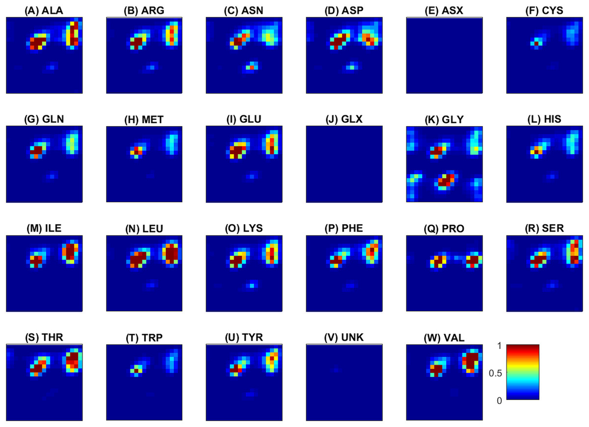
Figure 3: Torsion angles density maps (Ramachandran plots) averaged over all samples for each of the 20 standard and three non-standard (ASX, GLX, UNK) amino acids shown in alphabetical order from (A) to (W).
The horizontal and vertical axes at each plot correspond to ϕ and ψ angles and vary from −180∘ (top left) to 180∘ (right bottom). The color scale (blue to red) is in the range [0, 1]. For an amino acid a, red means that the number of occurrences of the specific value (ϕ, ψ) in all observations of a (within and across proteins) is at least equal to the number of proteins. On the opposite, blue indicates a small number of occurrences, and is observed for rare amino acids or unfavorable conformations. (A) ALA, (B) ARG, (C) ASN, (D) ASP, (E) ASX, (F) CYS, (G) GLN, (H) MET, (I) GLU, (J) GLX, (K) GLY, (L) HIS, (M) ILE, (N) LEU, (O) LYS, (P) PHE, (Q) PRO, (R) SER, (S) THR, (T) TRP, (U) TYR, (V) UNK, (W) VAL.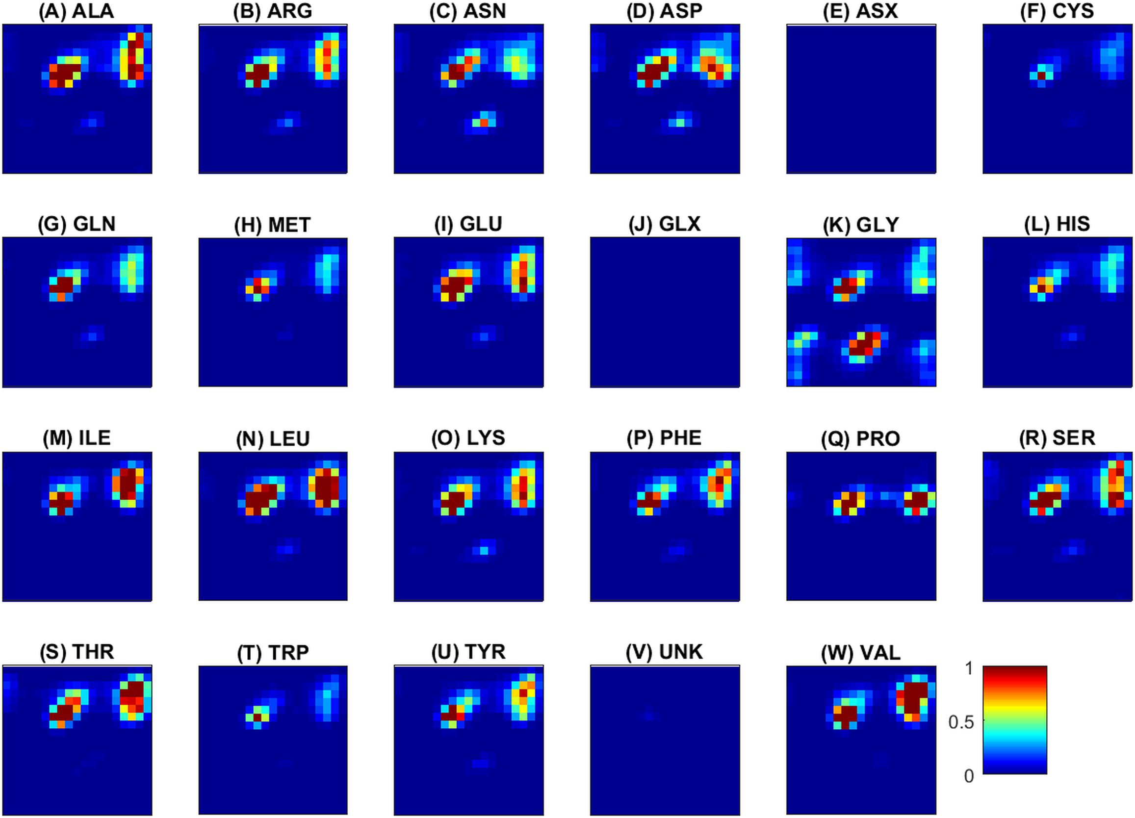
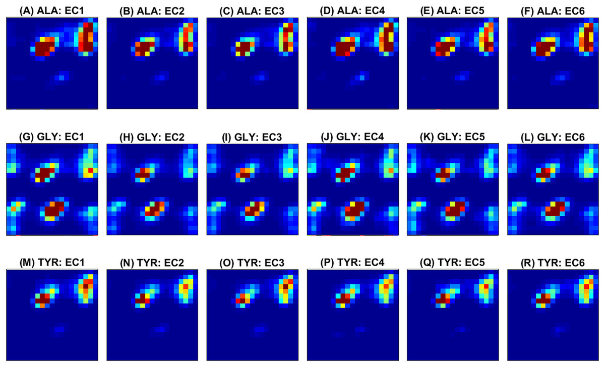
Figure 4: Ramachandran plots averaged across samples within each class.
Rows correspond to amino acids and columns to functional classes. Three amino acids (ALA from (A) to (F), GLY from (G) to (L) and TYR from (M) to (R)) are randomly selected for illustration of class separability. The horizontal and vertical axes at each plot correspond to ϕ and ψ angles and vary from −180∘ (top left) to 180∘ (right bottom). The color scale (blue to red) is in the range [0, 1] as illustrated in Fig. 3.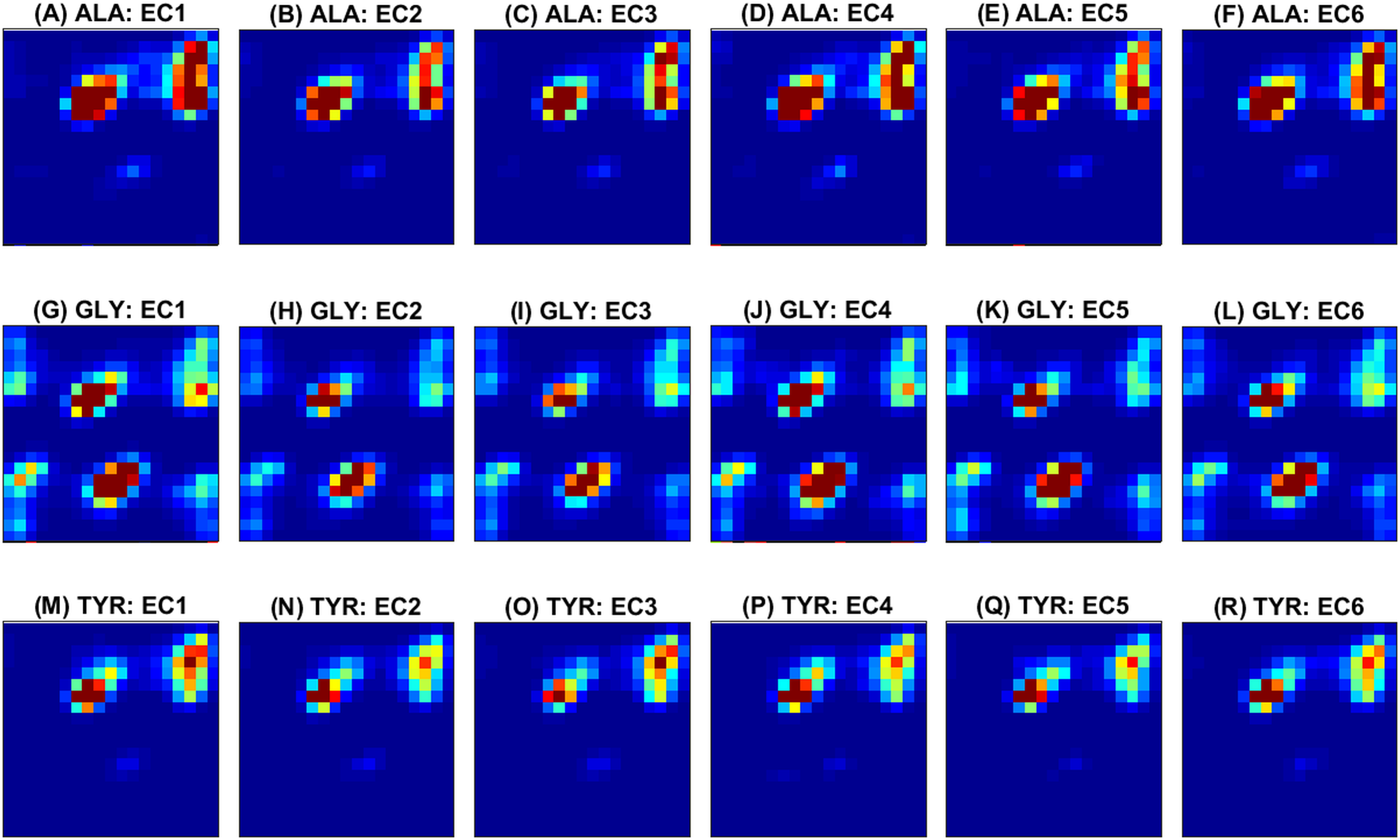
Examples of features maps representing amino acid distances (XD) are illustrated in Figs. 1 and 5. Figure 1 illustrates an image slice across the 3rd dimension, i.e., one [m × m] channel, and as introduced in the 2D multichannel CNN, i.e., after mean-centering (over all samples). Figure 5 illustrates image slices (of size [m × hD]) across the 1st dimension averaged within each class. Figure 5 has been produced by selecting the same amino acids as in Fig. 4 for ease of comparison of the different feature representations. It can be noticed that for all classes most pairwise distances are concentrated in the last bin, corresponding to high distances between amino acids. Also, as expected there are differences in quantity of each amino acid, e.g., by focusing on the last bin, it can be seen that ALA and GLY have higher values than TYR in most classes. Moreover, the feature maps indicate clear differences between samples of different classes.
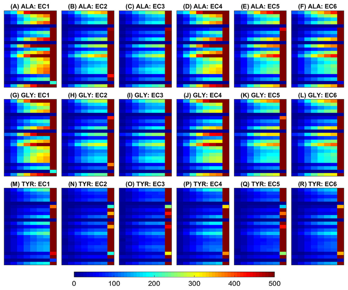
Figure 5: Histograms of paiwise amino acid distances averaged across samples within each class.
The same three amino acids selected in Fig. 4 are also shown here (ALA from (A) to (F), GLY from (G) to (L) and TYR from (M) to (R)). The horizontal axis at each plot represents the histogram bins (distance values in the range [5, 40]). The vertical axis at each plot corresponds to the 23 amino acids sorted alphabetically from top to bottom (ALA, ARG, ASN, ASP, ASX, CYS, GLN, MET, GLU, GLX, GLY, HIS, ILE, LEU, LYS, PHE, PRO, SER, THR, TRP, TYR, UNK, VAL). Thus each row shows the histogram of distances for a specific pair of the amino acids (the one in the title and the one corresponding to the specific row). The color scale is the same for all plots and is shown horizontally at the bottom of the figure.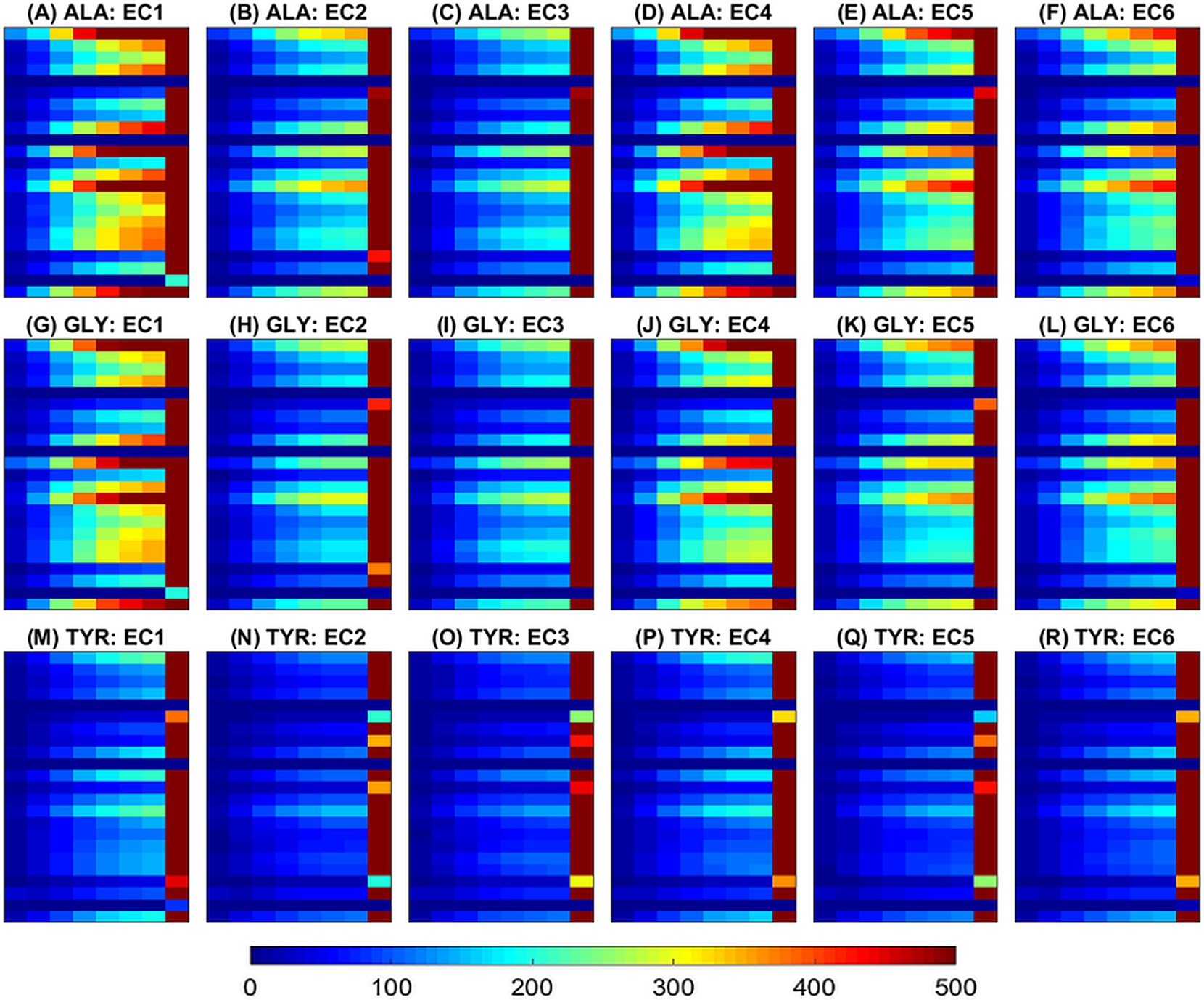
The discrimination ability and complementary of the extracted features in respect to classification performance is shown in Table 3. It can be observed that the relative position of amino acids and their arrangement in space (features XD) predict enzymatic function better than the backbone conformation (features XA). Also, the fusion of network decisions based on correlation distance outperforms predictions from either network alone, but the difference is only marginal in respect to the predictions by XD. In all cases the differences in prediction for the performed experiments (during cross validation) was very small (usually standard deviation <0.5%), indicating that the method is robust to variations in training examples.
| Feature sets | Linear-SVM | kNN |
|---|---|---|
| XA (angles) | 79.6 ± 0.5 | 82.4 ± 0.4 |
| XD (distances) | 88.1 ± 0.4 | 89.8 ± 0.2 |
| Ensemble | 88.0 ± 0.4 | 90.1 ± 0.2 |
Discussion
A deep CNN ensemble was presented that performs enzymatic function classification through fusion in feature level and decision level. The method has been applied for the prediction of the primary EC number and achieved 90.1% accuracy, which is a considerable improvement over the accuracy obtained in our previous work (73.5% in Amidi et al. (2016) and 83% in Amidi et al. (2017)) when only structural information was incorporated. These results were achieved without imposing any pre-selection criteria, such as based on sequence identity, thus the effect of evolutionary relationships, as confounding factor in the prediction of function from 3D structure, has not been sufficiently studied. Since deep learning technology requires a large number of samples to produce generalizable models, a filtered dataset with only non-redundant proteins would be too small for reliable training. This is a limitation of the current approach, which mainly aimed to increase predictive power over previous methods using common features for structural representation and common classifiers such as SVM and nearest neighbor, rather than addressing this confounding factor in the prediction of protein structure.
Many methods have been proposed in the literature using different features and different classifiers. Nasibov & Kandemir-Cavas (2009) obtained 95%–99% accuracy by applying kNN-based classification on 1200 enzymes based on their amino acid composition. Shen & Chou (2007) fused results derived from the functional domain and evolution information and obtained 93.7% average accuracy on 9,832 enzymes. On the same dataset, Wang et al. (2011) improved the accuracy (which ranged from 81% to 98% when predicting the first three EC digits) by using sequence encoding and SVM for hierarchy labels. Kumar & Choudhary (2012) reported overall accuracy of 87.7% in predicting the main class for 4,731 enzymes using random forests. Volpato, Adelfio & Pollastri (2013) applied neural networks on the full sequence and achieve 96% correct classification on 6,000 non-redundant proteins. Most of the previous methods incorporate sequence-based features. Many were assessed on a subset of enzymes acquired after imposition of different pre-selection criteria and levels of sequence similarity. More discussion on machine learning techniques for single-label and multi-label enzyme classification can be found in Amidi et al. (2017).
Assessment of the relationship between function and structure (Todd, Orengo & Thornton, 2001) revealed 95% conservation of the fourth EC digit for proteins with up to 30% sequence identity. Similarity, Devos & Valencia (2000) concluded that enzymatic function is mostly conserved for the first digit of EC code whereas more detailed functional characteristics are poorly conserved. It is generally believed that as sequences diverge, 3D protein structure becomes a more reliable predictor than sequence, and that structure is far more conserved than sequence in nature (Illergård, Ardell & Elofsson, 2009). The focus of this study was to explore the predictive ability of 3D structure and provide a tool that can generalize in cases where sequence information is insufficient. Thus, the presented results are not directly comparable to the ones of previous methods due to the use of different features and datasets. If desired, the current approach can easily incorporate also sequence-related features. In such a case however, the use of non-homologous data would be inevitable for rigorous assessment.
The reported accuracy is the average of five folds on the testing set. A separate validation set was not used within each fold, because the design of the network architecture (size of convolution kernel, number of layers, etc.) and the final classifier (number of neighbors in kNN) were preselected and not optimized within the learning framework. Additional validation and optimization of the model would be necessary to improve performance and provide better insight into the capabilities of this method.
A possible limitation of the proposed approach is that the extracted features do not capture the topological properties of the 3D structure. Due to the statistical nature of the implemented descriptors, which were calculated by considering the amino acids as elements in Euclidean space, connectivity information is not strictly retained. The author and colleagues recently started to investigate in parallel the predictive power of the original 3D structure, represented as a volumetric image, without the extraction of any statistical features. Since the more detailed representation increased the dimensionality considerably, new ways are being explored to optimally incorporate the relationship between the structural units (amino-acids) in order not to impede the learning process.
Conclusions
A method was presented that extracts shape features from the 3D protein geometry that are introduced into a deep CNN ensemble for enzymatic function prediction. The investigation of protein function based only on structure reveals relationships hidden at the sequence level and provides the foundation to build a better understanding of the molecular basis of biological complexity. Overall, the presented approach can provide quick protein function predictions on extensive datasets opening the path for relevant applications, such as pharmacological target identification. Future work includes application of the method for prediction of the hierarchical relation of function subcategories and annotation of enzymes up to the last digit of the enzyme classification system.