
Two-dimensional Kolmogorov complexity and an empirical validation of the Coding theorem method by compressibility
- Published
- Accepted
- Received
- Academic Editor
- Mikael Skoglund
- Subject Areas
- Computational Biology, Artificial Intelligence, Theory and Formal Methods
- Keywords
- Algorithmic complexity, Algorithmic probability, Kolmogorov–Chaitin complexity, Algorithmic information theory, Cellular automata, Solomonoff–Levin universal distribution, Information theory, Dimensional complexity, Image complexity, Small Turing machines
- Copyright
- © 2015 Zenil et al.
- Licence
- This is an open access article distributed under the terms of the Creative Commons Attribution License, which permits unrestricted use, distribution, reproduction and adaptation in any medium and for any purpose provided that it is properly attributed. For attribution, the original author(s), title, publication source (PeerJ Computer Science) and either DOI or URL of the article must be cited.
- Cite this article
- 2015. Two-dimensional Kolmogorov complexity and an empirical validation of the Coding theorem method by compressibility. PeerJ Computer Science 1:e23 https://doi.org/10.7717/peerj-cs.23
Abstract
We propose a measure based upon the fundamental theoretical concept in algorithmic information theory that provides a natural approach to the problem of evaluating n-dimensional complexity by using an n-dimensional deterministic Turing machine. The technique is interesting because it provides a natural algorithmic process for symmetry breaking generating complex n-dimensional structures from perfectly symmetric and fully deterministic computational rules producing a distribution of patterns as described by algorithmic probability. Algorithmic probability also elegantly connects the frequency of occurrence of a pattern with its algorithmic complexity, hence effectively providing estimations to the complexity of the generated patterns. Experiments to validate estimations of algorithmic complexity based on these concepts are presented, showing that the measure is stable in the face of some changes in computational formalism and that results are in agreement with the results obtained using lossless compression algorithms when both methods overlap in their range of applicability. We then use the output frequency of the set of 2-dimensional Turing machines to classify the algorithmic complexity of the space-time evolutions of Elementary Cellular Automata.
Introduction
The question of natural measures of complexity for objects other than strings and sequences, in particular suited for 2-dimensional objects, is an open important problem in complexity science and with potential applications to molecule folding, cell distribution, artificial life and robotics. Here we provide a measure based upon the fundamental theoretical concept that provides a natural approach to the problem of evaluating n-dimensional algorithmic complexity by using an n-dimensional deterministic Turing machine, popularized under the term of Turmites for n = 2, from which the so-called Langton’s ant is an example of a Turing universal Turmite. A series of experiments to validate estimations of Kolmogorov complexity based on these concepts is presented, showing that the measure is stable in the face of some changes in computational formalism and that results are in agreement with the results obtained using lossless compression algorithms when both methods overlap in their range of applicability. We also present a divide and conquer algorithm that we call Block Decomposition Method (BDM) application to classification of images and space–time evolutions of discrete systems, providing evidence of the soundness of the method as a complementary alternative to compression algorithms for the evaluation of algorithmic complexity. We provide exact numerical approximations of Kolmogorov complexity of square image patches of size 3 and more, with the BDM allowing scalability to larger 2-dimensional arrays and even greater dimensions.
The challenge of finding and defining 2-dimensional complexity measures has been identified as an open problem of foundational character in complexity science (Feldman & Crutchfield, 2003; Shalizi, Shalizi & Haslinger, 2004). Indeed, for example, humans understand 2-dimensional patterns in a way that seems fundamentally different than 1-dimensional (Feldman, 2008). These measures are important because current 1-dimensional measures may not be suitable to 2-dimensional patterns for tasks such as quantitatively measuring the spatial structure of self-organizing systems. On the one hand, the application of Shannon’s Entropy and Kolmogorov complexity has traditionally been designed for strings and sequences. However, n-dimensional objects may have structure only distinguishable in their natural dimension and not in lower dimensions. This is indeed a question related to the loss of information in dimension reductionality (Zenil, Kiani & Tegnér, in press). A few measures of 2-dimensional complexity have been proposed before building upon Shannon’s entropy and block entropy (Feldman & Crutchfield, 2003; Andrienko, Brilliantov & Kurths, 2000), mutual information and minimal sufficient statistics (Shalizi, Shalizi & Haslinger, 2004) and in the context of anatomical brain MRI analysis (Young et al., 2009; Young & Schuff, 2008). A more recent application, also in the medical context related to a measure of consciousness, was proposed using lossless compressibility for EGG brain image analysis was proposed in Casali et al. (2013).
On the other hand, for Kolmogorov complexity, the common approach to evaluating the algorithmic complexity of a string has been by using lossless compression algorithms because the length of lossless compression is an upper bound of Kolmogorov complexity. Short strings, however, are difficult to compress in practice, and the theory does not provide a satisfactory solution to the problem of the instability of the measure for short strings.
Here we use so-called Turmites (2-dimensional Turing machines) to estimate the Kolmogorov complexity of images, in particular space–time diagrams of cellular automata, using Levin’s Coding theorem from algorithmic probability theory. We study the problem of the rate of convergence by comparing approximations to a universal distribution using different (and larger) sets of small Turing machines and comparing the results to that of lossless compression algorithms carefully devising tests at the intersection of the application of compression and algorithmic probability. We found that strings which are more random according to algorithmic probability also turn out to be less compressible, while less random strings are clearly more compressible.
Compression algorithms have proven to be signally applicable in several domains (see e.g., Li & Vitányi, 2009), yielding surprising results as a method for approximating Kolmogorov complexity. Hence their success is in part a matter of their usefulness. Here we show that an alternative (and complementary) method yields compatible results with the results of lossless compression. For this we devised an artful technique by grouping strings that our method indicated had the same program-size complexity, in order to construct files of concatenated strings of the same complexity (while avoiding repetition, which could easily be exploited by compression). Then a lossless general compression algorithm was used to compress the files and ascertain whether the files that were more compressed were the ones created with highly complex strings according to our method. Similarly, files with low Kolmogorov complexity were tested to determine whether they were better compressed. This was indeed the case, and we report these results in ‘Validation of the Coding Theorem Method by Compressibility’. In ‘Comparison of Km and compression of cellular automata’ we also show that the Coding theorem method yields a very similar classification of the space–time diagrams of Elementary Cellular Automata, despite the disadvantage of having used a limited sample of a Universal Distribution. In all cases the statistical evidence is strong enough to suggest that the Coding theorem method is sound and capable of producing satisfactory results. The Coding theorem method also represents the only currently available method for dealing with very short strings and in a sense is an expensive but powerful “microscope” for capturing the information content of very small objects.
Kolmogorov–Chaitin complexity
Central to algorithmic information theory (AIT) is the definition of algorithmic (Kolmogorov–Chaitin or program-size) complexity (Kolmogorov, 1965; Chaitin, 1969): (1)
That is, the length of the shortest program p that outputs the string s running on a universal Turing machine T. A classic example is a string composed of an alternation of bits, such as (01)n, which can be described as “n repetitions of 01”. This repetitive string can grow fast while its description will only grow by about log2(n). On the other hand, a random-looking string such as 011001011010110101 may not have a much shorter description than itself.
Uncomputability and instability of K
A technical inconvenience of K as a function taking s to the length of the shortest program that produces s is its uncomputability (Chaitin, 1969). In other words, there is no program which takes a string s as input and produces the integer K(s) as output. This is usually considered a major problem, but one ought to expect a universal measure of complexity to have such a property. On the other hand, K is more precisely upper semi-computable, meaning that one can find upper bounds, as we will do by applying a technique based on another semi-computable measure to be presented in the ‘Solomonoff–Levin Algorithmic Probability’.
The invariance theorem guarantees that complexity values will only diverge by a constant c (e.g., the length of a compiler, a translation program between U1 and U2) and that they will converge at the limit.
Invariance Theorem (Calude, 2002; Li & Vitányi, 2009): If U1 and U2 are two universal Turing machines and KU1(s) and KU2(s) the algorithmic complexity of s for U1 and U2, there exists a constant c such that for all s: (2)
Hence the longer the string, the less important c is (i.e., the choice of programming language or universal Turing machine). However, in practice c can be arbitrarily large because the invariance theorem tells nothing about the rate of convergence between KU1 and KU2 for a string s of increasing length, thus having an important impact on short strings.
Solomonoff–Levin Algorithmic Probability
The algorithmic probability (also known as Levin’s semi-measure) of a string s is a measure that describes the expected probability of a random program p running on a universal (prefix-free1) Turing machine T producing s upon halting. Formally (Solomonoff, 1964; Levin, 1974; Chaitin, 1969), (3)
Levin’s semi-measure2 m(s) defines a distribution known as the Universal Distribution (a beautiful introduction is given in Kircher, Li & Vitanyi (1997)). It is important to notice that the value of m(s) is dominated by the length of the smallest program p (when the denominator is larger). However, the length of the smallest p that produces the string s is K(s). The semi-measure m(s) is therefore also uncomputable, because for every s, m(s) requires the calculation of 2−K(s), involving K, which is itself uncomputable. An alternative to the traditional use of compression algorithms is the use of the concept of algorithmic probability to calculate K(s) by means of the following theorem.
Coding Theorem (Levin, 1974): (4)
This means that if a string has many descriptions it also has a short one. It beautifully connects frequency to complexity, more specifically the frequency of occurrence of a string with its algorithmic (Kolmogorov) complexity. The Coding theorem implies that (Cover & Thomas, 2006; Calude, 2002) one can calculate the Kolmogorov complexity of a string from its frequency (Delahaye & Zenil, 2007b; Delahaye & Zenil, 2007a; Zenil, 2011; Delahaye & Zenil, 2012), simply rewriting the formula as: (5)
An important property of m as a semi-measure is that it dominates any other effective semi-measure μ, because there is a constant cμ such that for all s, m(s) ≥ cμμ(s). For this reason m(s) is often called a Universal Distribution (Kircher, Li & Vitanyi, 1997).
The Coding Theorem method
Let D(n, m) be a function (Delahaye & Zenil, 2012) defined as follows: (6) where (n, m) denotes the set of Turing machines with n states and m symbols, running with empty input, and |A| is, in this case, the cardinality of the set A. In Zenil (2011) and Delahaye & Zenil (2012) we calculated the output distribution of Turing machines with 2-symbols and n = 1, …, 4 states for which the Busy Beaver (Radó, 1962) values are known, in order to determine the halting time, and in Soler-Toscano et al. (2014) results were improved in terms of number and Turing machine size (5 states) and in the way in which an alternative to the Busy Beaver information was proposed, hence no longer needing exact information of halting times in order to approximate an informative distribution.
Here we consider an experiment with 2-dimensional deterministic Turing machines (also called Turmites) in order to estimate the Kolmogorov complexity of 2-dimensional objects, such as images that can represent space–time diagrams of simple systems. A Turmite is a Turing machine which has an orientation and operates on a grid for “tape”. The machine can move in 4 directions rather than in the traditional left and right movements of a traditional Turing machine head. A reference to this kind of investigation and definition of 2D Turing machines can be found in Wolfram (2002), one popular and possibly one of the first examples of this variation of a Turing machine is Lagton’s ant (Langton, 1986) also proven to be capable of Turing-universal computation.
In ‘Comparison of Km and approaches based on compression’, we will use the so-called Turmites to provide evidence that Kolmogorov complexity evaluated through algorithmic probability is consistent with the other (and today only) method for approximating K, namely lossless compression algorithms. We will do this in an artful way, given that compression algorithms are unable to compress strings that are too short, which are the strings covered by our method. This will involve concatenating strings for which our method establishes a Kolmogorov complexity, which then are given to a lossless compression algorithm in order to determine whether it provides consistent estimations, that is, to determine whether strings are less compressible where our method says that they have greater Kolmogorov complexity and whether strings are more compressible where our method says they have lower Kolmogorov complexity. We provide evidence that this is actually the case.
In ‘Comparison of Km and compression of cellular automata’ we will apply the results from the Coding theorem method to approximate the Kolmogorov complexity of 2-dimensional evolutions of 1-dimensional, closest neighbor Cellular Automata as defined in Wolfram (2002), and by way of offering a contrast to the approximation provided by a general lossless compression algorithm (Deflate). As we will see, in all these experiments we provide evidence that the method is just as successful as compression algorithms, but unlike the latter, it can deal with short strings.
Deterministic 2-dimensional Turing machines (Turmites)
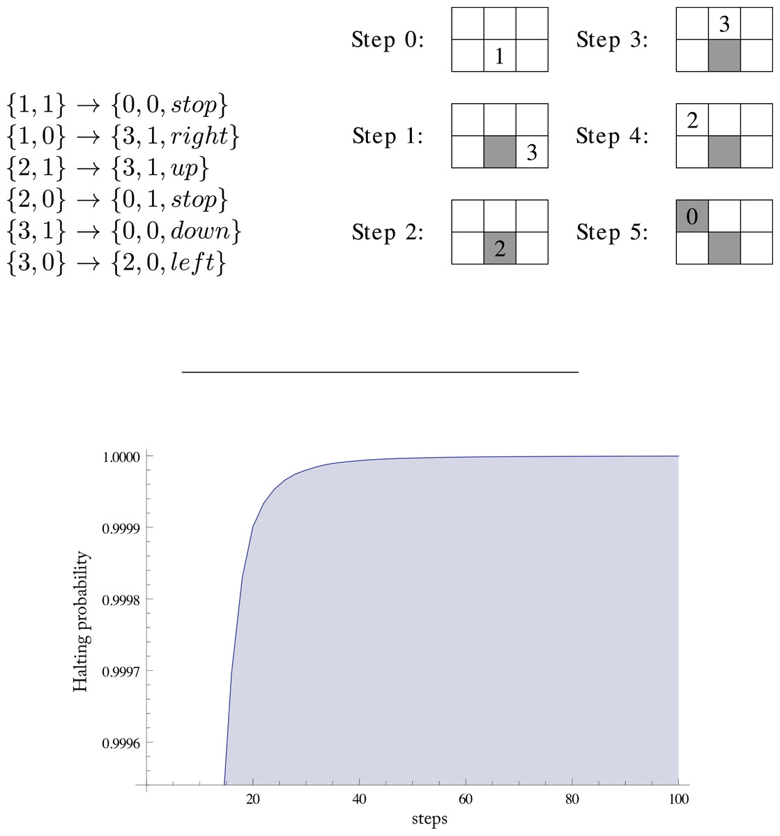
Turmites or 2-dimensional (2D) Turing machines run not on a 1-dimensional tape but in a 2-dimensional unbounded grid or array. At each step they can move in four different directions (up, down, left, right) or stop. Transitions have the format {n1, m1} → {n2, m2, d}, meaning that when the machine is in state n1 and reads symbols m1, it writes m2, changes to state n2 and moves to a contiguous cell following direction d. If n2 is the halting state then d is stop. In other cases, d can be any of the other four directions.
Let (n, m)2D be the set of Turing machines with n states and m symbols. These machines have nm entries in the transition table, and for each entry {n1, m1} there are 4nm + m possible instructions, that is, m different halting instructions (writing one of the different symbols) and 4nm non-halting instructions (4 directions, n states and m different symbols). So the number of machines in (n, m)2D is (4nm + m)nm. It is possible to enumerate all these machines in the same way as 1D Turing machines (e.g., as has been done in Wolfram (2002) and Joosten (2012)). We can assign one number to each entry in the transition table. These numbers go from 0 to 4nm + m − 1 (given that there are 4nm + m different instructions). The numbers corresponding to all entries in the transition table (irrespective of the convention followed in sorting them) form a number with nm digits in base 4nm + m. Then, the translation of a transition table to a natural number and vice versa can be done through elementary arithmetical operations.
We take as output for a 2D Turing machine the minimal array that includes all cells visited by the machine. Note that this probably includes cells that have not been visited, but it is the more natural way of producing output with some regular format and at the same time reducing the set of different outputs.
Figure 1 shows an example of the transition table of a Turing machine in (3, 2)2D and its execution over a ‘0’-filled grid. We show the portion of the grid that is returned as the output array. Two of the six cells have not been visited by the machine.
An Approximation to the Universal Distribution
We have run all machines in (4, 2)2D just as we have done before for deterministic 1-dimensional Turing machines (Delahaye & Zenil, 2012; Soler-Toscano et al., 2014). That is, considering the output of all different machines starting both in a ‘0’-filled grid (all white) and in a ‘1’-filled (all black) grid. Symmetries are described and used in the same way than in Soler-Toscano et al. (2014) in order to avoid running a larger number of machines whose output can be predicted from other equivalent machines (by rotation, transposition, 1-complementation, reversion, etc.) that produce equivalent outputs with the same frequency.
We also used a reduced enumeration to avoid running certain trivial machines whose behavior can be predicted from the transition table, as well as filters to detect non-halting machines before exhausting the entire runtime. In the reduced enumeration we considered only machines with an initial transition moving to the right and changing to a different state than the initial and halting states. Machines moving to the initial state at the starting transition run forever, and machines moving to the halting state produce single-character output. So we reduce the number of initial transitions in (n, m)2D to m(n − 1) (the machine can write any of the m symbols and change to any state in {2, …, n}). The set of different machines is reduced accordingly to k(n − 1)(4nm + m)nm−1. To enumerate these machines we construct a mixed-radix number, given that the digit corresponding to the initial transition now goes from 0 to m(n − 1) − 1. To the output obtained when running this reduced enumeration we add the single-character arrays that correspond to machines moving to the initial state at the starting transition. These machines and their output can be easily quantified. Also, to take into account machines with the initial transition moving in a different direction than the right one, we consider the 90, 180 and 270 degree rotations of the strings produced, given that for any machine moving up (left/down) at the initial transition, there is another one moving right that produces the identical output but rotates −90 (−180/−270) degrees.
Setting the runtime
The Busy Beaver runtime value for (4, 2) is 107 steps upon halting. But no equivalent Busy Beavers are known for 2-dimensional Turing machines (although variations of Turmite’s Busy Beaver functions have been proposed (Pegg, 2013)). So to set the runtime in our experiment we generated a sample of 334 × 108 random machines in the reduced enumeration. We used a runtime of 2,000 steps for the runtime sample, this is 10.6% of the machines in the reduced enumeration for (4, 2)2D, but 1,500 steps for running all (4, 2)2D. These machines were generated instruction by instruction. As we have explained above, it is possible to assign a natural number to every instruction. So to generate a random machine in the reduced enumeration for (n, m)2D we produce a random number from 0 to m(n − 1) − 1 for the initial transition and from 0 to 4nm + m − 1 for the other nm − 1 transitions. We used the implementation of the Mersenne Twister in the Boost C++ library. The output of this sample was the distribution of the runtime of the halting machines.
Figure 1 shows the probability that a random halting machine will halt in at most the number of steps indicated on the horizontal axis. For 100 steps this probability is 0.9999995273. Note that the machines in the sample are in the reduced enumeration, a large number of very trivial machines halting in just one step having been removed. So in the complete enumeration the probability of halting in at most 100 steps is even greater.
But we found some high runtime values—precisely 23 machines required more than 1,000 steps. The highest value was a machine progressing through 1,483 steps upon halting. So we have enough evidence to believe that by setting the runtime at 2,000 steps we have obtained almost all (if not all) output arrays. We ran all 6 × 347 Turing machines in the reduced enumeration for (4, 2)2D. Then we applied the completions explained before.
Output analysis
The final output represents the result of 2(4nm + m)2 executions (all machines in (4, 2)2D starting with both blank symbols ‘0’ and ‘1’). We found 3,079,179,980,224 non-halting machines and 492,407,829,568 halting machines. A number of 1,068,618 different binary arrays were produced after 12 days of calculation with a supercomputer of medium size (a 25×86-64 CPUs running at 2,128 MHz each with 4 GB of memory each, located at the Centro Informático Científico de Andalucía (CICA), Spain.
Let D(4, 2)2D be the set constructed by dividing the occurrences of each different array by the number of halting machines as a natural extension of Eq. (6) for 2-dimensional Turing machines. Then, for every string s, (7) using the Coding theorem (Eq. (3)). Figure 2 shows the top 36 objects in D(4, 2)2D, that is the objects with lowest Kolmogorov complexity values.
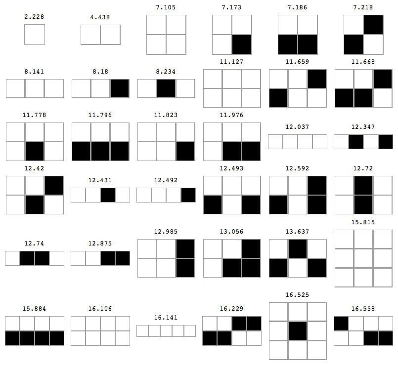
Figure 2: The top 36 objects in D(4, 2)2D preceded by their Km,2D values, sorted by higher to lower frequency and therefore from smaller to larger Kolmogorov complexity after application of the Coding theorem.
Only non-symmetrical cases are displayed. The grid is only for illustration purposes.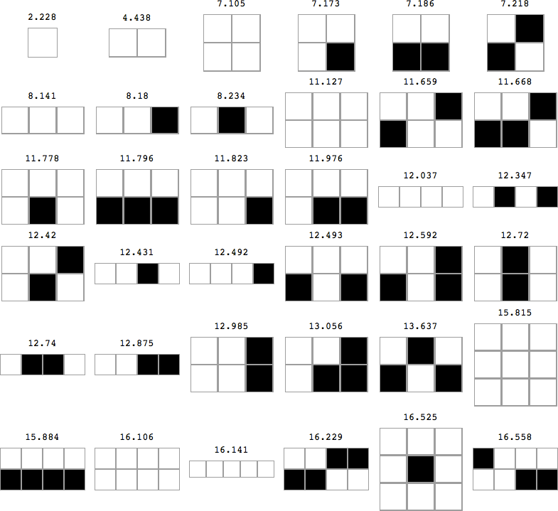
Evaluating 2-dimensional Kolmogorov complexity
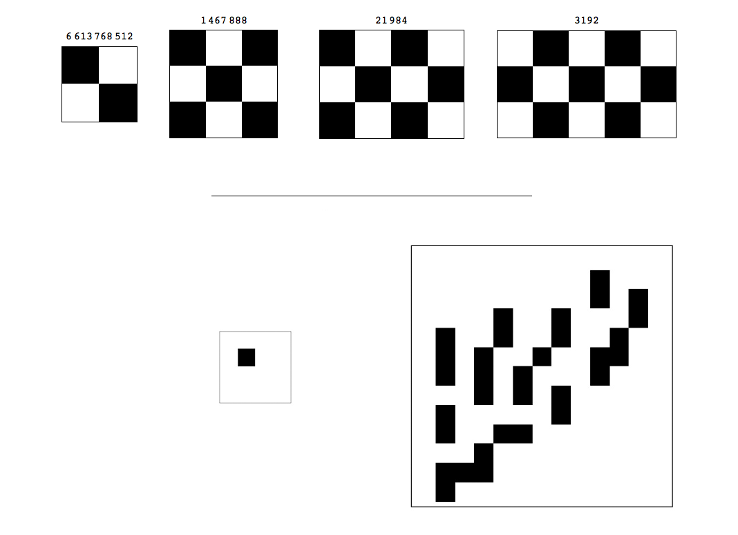
D(4, 2)2D denotes the frequency distribution (a calculated Universal Distribution) from the output of deterministic 2-dimensional Turing machines, with associated complexity measure Km,2D. D(4, 2)2D distributes 1,068,618 arrays into 1,272 different complexity values, with a minimum complexity value of 2.22882 bits (an explanation of non-integer program-size complexity is given in Soler-Toscano et al. (2014) and Soler-Toscano et al. (2013)), a maximum value of 36.2561 bits and a mean of 35.1201. Considering the number of possible square binary arrays given by the formula 2d×d (without considering any symmetries), D(4, 2)2D can be said to produce all square binary arrays of length up to 3 × 3, that is square arrays, and 60,016 of the 2(4×4) = 65,536 square arrays with side of length (or dimension) d = 4. It only produces 84,104 of the 33,554,432 possible square binary arrays of length d = 5 and only 11,328 of the possible 68,719,476,736 of dimension d = 6. The largest square array produced in D(4, 2)2D is of side length d = 13 (Left of Fig. 3) out of a possible 748 × 1048; it has a Km,2D value equal to 34.2561.

What one would expect from a distribution where simple patterns are more frequent (and therefore have lower Kolmogorov complexity after application of the Coding theorem) would be to see patterns of the “checkerboard” type with high frequency and low random complexity (K), and this is exactly what we found (see Fig. 3), while random looking patterns were found at the bottom among the least frequent ones (Fig. 4).
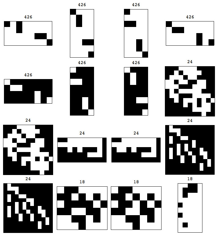
Figure 4: Symmetry breaking from fully deterministic symmetric computational rules.
Bottom 16 objects in the classification with lowest frequency, or being most random according to D(4, 2)2D. It is interesting to note the strong similarities given that similar-looking cases are not always exact symmetries. The arrays are preceded by the number of occurrences of production from all the (4, 2)2D Turing machines.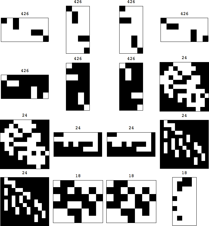
We have coined the informal notion of a “climber” as an object in the frequency classification (from greatest to lowest frequency) that appears better classified among objects of smaller size rather than with the arrays of their size, this is in order to highlight possible candidates for low complexity, hence illustrating how the process make low complexity patterns to emerge. For example, “checkerboard” patterns (see Fig. 3) seem to be natural “climbers” because they come significantly early (more frequent) in the classification than most of the square arrays of the same size. In fact, the larger the checkerboard array, the more of a climber it seems to be. This is in agreement with what we have found in the case of strings (Zenil, 2011; Delahaye & Zenil, 2012; Soler-Toscano et al., 2014) where patterned objects emerge (e.g., (01)n, that is, the string 01 repeated n times), appearing relatively increasingly higher in the frequency classifications the larger n is, in agreement with the expectation that patterned objects should also have low Kolmogorov complexity.
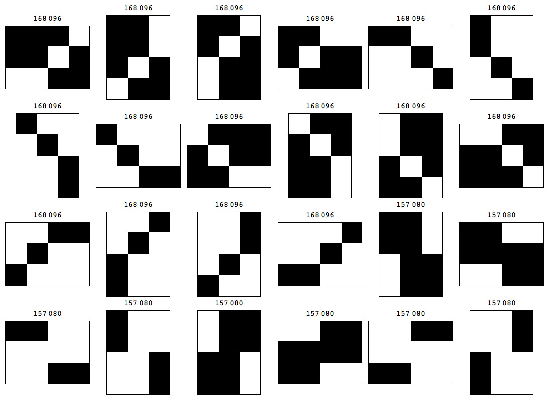
Figure 5: Two “climbers” (and all their symmetric cases) found in D(4, 2)2D.
Symmetric objects have higher frequency and therefore lower Kolmogorov complexity. Nevertheless, a fully deterministic algorithmic process starting from completely symmetric rules produces a range of patterns of high complexity and low symmetry.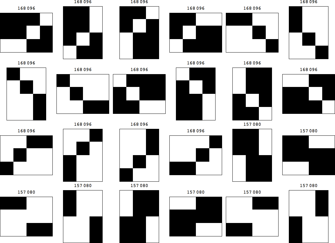
An attempt of a definition of a climber is a pattern P of size a × b with small complexity among all a × b patterns, such that there exists smaller patterns Q (say c × d, with cd < ab) such that Km(P) < Km(Q) < median(Km(all ab patterns)).
For example, Fig. 5 shows arrays that come together among groups of much shorter arrays, thereby demonstrating, as expected from a measure of randomness, that array—or string—size is not what determines complexity (as we have shown before in Zenil (2011), Delahaye & Zenil (2012) and Soler-Toscano et al. (2014) for binary strings). The fact that square arrays may have low Kolmogorov complexity can be understood in several ways, some of which strengthen the intuition that square arrays should be less Kolmogorov random, such as for example, the fact that for square arrays one only needs the information of one of its dimensions to determine the other, either height or width.
Figure 5 shows cases in which square arrays are significantly better classified towards the top than arrays of similar size. Indeed, 100% of the squares of size 2 × 2 are in the first fifth (F1), as are the 3 × 3 arrays. Square arrays of 4 × 4 are distributed as follows when dividing (4, 2)2D in 5 equal parts: 72.66%, 15.07%, 6.17359%, 2.52%, 3.56%.
Figure 6: Complete reduced set (non-symmetrical cases under reversion and complementation) of 3 × 3 patches in Km,2D sorted from lowest to greatest Kolmogorov complexity after application of the Coding theorem (Eq. (3)) to the output frequency of 2-D Turing machines.
We denote this set by Km,2D3×3. For example, the 2 glider configurations in the Game of Life (Gardner, 1970) come with high Kolmogorov complexity (with approximated values of 20.2261 and 20.5031).
Validation of the Coding Theorem Method by compressibility
One way to validate our method based on the Coding theorem (Eq. (3)) is to attempt to measure its departure from the compressibility approach. This cannot be done directly, for as we have explained, compression algorithms perform poorly on short strings, but we did find a way to partially circumvent this problem by selecting subsets of strings for which our Coding theorem method calculated a high or low complexity which were then used to generate a file of length long enough to be compressed.
Comparison of Km and approaches based on compression
It is also not uncommon to detect instabilities in the values retrieved by a compression algorithm for short strings, as explained in ‘Uncomputability and instability of K’, strings which the compression algorithm may or may not compress. This is not a malfunction of a particular lossless compression algorithm (e.g., Deflate, used in most popular computer formats such as ZIP and PNG) or its implementation, but a commonly encountered problem when lossless compression algorithms attempt to compress short strings.
When researchers have chosen to use compression algorithms for reasonably long strings, they have proven to be of great value, for example, for DNA false positive repeat sequence detection in genetic sequence analysis (Rivals et al., 1996), in distance measures and classification methods (Cilibrasi & Vitanyi, 2005), and in numerous other applications (Li & Vitányi, 2009). However, this effort has been hamstrung by the limitations of compression algorithms–currently the only method used to approximate the Kolmogorov complexity of a string–given that this measure is not computable.
In this section we study the relation between Km and approaches to Kolmogorov complexity based on compression. We show that both approaches are consistent, that is, strings with higher Km value are less compressible than strings with lower values. This is as much validation of Km and our Coding theorem method as it is for the traditional lossless compression method as approximation techniques to Kolmogorov complexity. The Coding theorem method is, however, especially useful for short strings where losses compression algorithms fail, and the compression method is especially useful where the Coding theorem is too expensive to apply (long strings).
Compressing strings of length 10–15
For this experiment we have selected the strings in D(5) with lengths ranging from 10 to 15. D(5) is the frequency distribution of strings produced by all 1-dimensional deterministic Turing machines as described in Soler-Toscano et al. (2014). Table 1 shows the number of D(5) strings with these lengths. Up to length 13 we have almost all possible strings. For length 14 we have a considerable number and for length 15 there are less than 50% of the 215 possible strings. The distribution of complexities is shown in Fig. 7.
| Length (l) | Strings |
|---|---|
| 10 | 1,024 |
| 11 | 2,048 |
| 12 | 4,094 |
| 13 | 8,056 |
| 14 | 13,068 |
| 15 | 14,634 |
As expected, the longer the strings, the greater their average complexity. The overlapping of strings with different lengths that have the same complexity correspond to climbers. The experiment consisted in creating files with strings of different Km-complexity but equal length (files with more complex (random) strings are expected to be less compressible than files with less complex (random) strings). This was done in the following way. For each l (10 ≤ l ≤ 15), we let S(l) denote the list of strings of length l, sorted by increasing Km complexity. For each S(l) we made a partition of 10 sets with the same number of consecutive strings. Let’s call these partitions P(l, p), 1 ≤ p ≤ 10.
Then for each P(l, p) we have created 100 files, each with 100 random strings in P(l, p) in random order. We called these files F(l, p, f), 1 ≤ f ≤ 100. Summarizing, we now have:
-
6 different string lengths l, from 10 to 15, and for each length
-
10 partitions (sorted by increasing complexity) of the strings with length l, and
-
100 files with 100 random strings in each partition.
This makes for a total of 6,000 different files. Each file contains 100 different binary strings, hence with length of 100 × l symbols.
A crucial step is to replace the binary encoding of the files by a larger alphabet, retaining the internal structure of each string. If we compressed the files F(l, p, f) by using binary encoding then the final size of the resulting compressed files would depend not only on the complexity of the separate strings but on the patterns that the compressor discovers along the whole file. To circumvent this we chose two different symbols to represent the ‘0’ and ‘1’ in each one of the 100 different strings in each file. The same set of 200 symbols was used for all files. We were interested in using the most standard symbols we possibly could, so we created all pairs of characters from ‘a’ to ‘p’ (256 different pairs) and from this set we selected 200 two-character symbols that were the same for all files. This way, though we do not completely avoid the possibility of the compressor finding patterns in whole files due to the repetition of the same single character in different strings, we considerably reduce the impact of this phenomenon.
The files were compressed using the Mathematica function Compress, which is an implementation of the Deflate algorithm (Lempel–Ziv plus Huffman coding). Figure 7 shows the distributions of lengths of the compressed files for the different string lengths. The horizontal axis shows the 10 groups of files in increasing Km. As the complexity of the strings grows (right part of the diagrams), the compressed files are larger, so they are harder to compress. The relevant exception is length 15, but this is probably related to the low number of strings of that length that we have found, which are surely not the most complex strings of length 15.
We have used other compressors such as GZIP (which uses Lempel–Ziv algorithm LZ77) and BZIP2 (Burrows–Wheeler block sorting text compression algorithm and Huffman coding), with several compression levels. The results are similar to those shown in Fig. 7.
Comparing (4, 2)2D and (4, 2)
We shall now look at how 1-dimensional arrays (hence strings) produced by 2D Turing machines correlate with strings that we have calculated before (Zenil, 2011; Delahaye & Zenil, 2012; Soler-Toscano et al., 2014) (denoted by D(5)). In a sense this is like changing the Turing machine formalism to see whether the new distribution resembles distributions following other Turing machine formalisms, and whether it is robust enough.
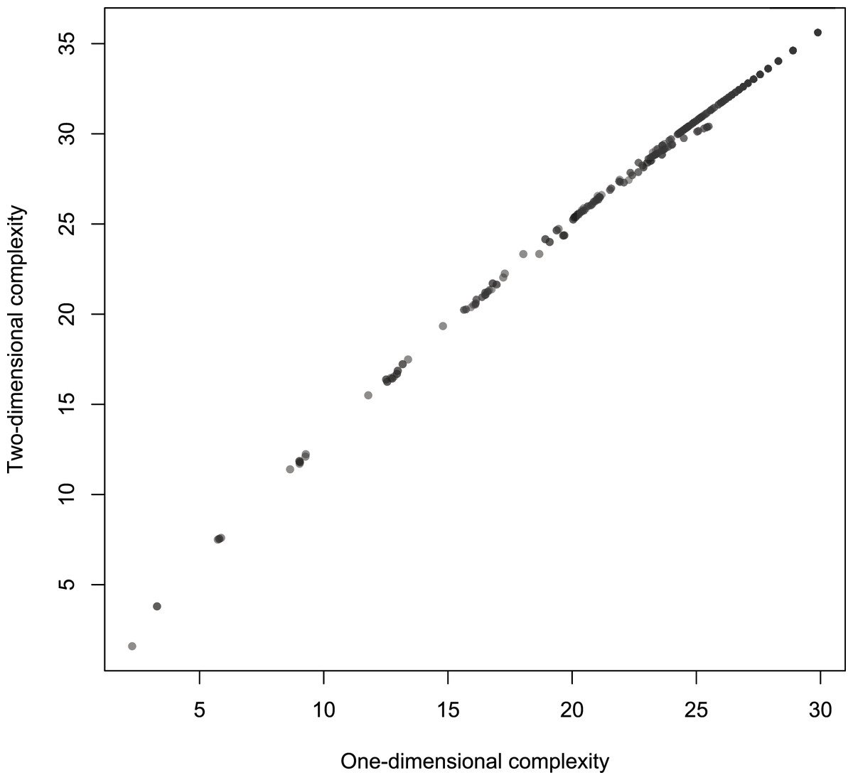
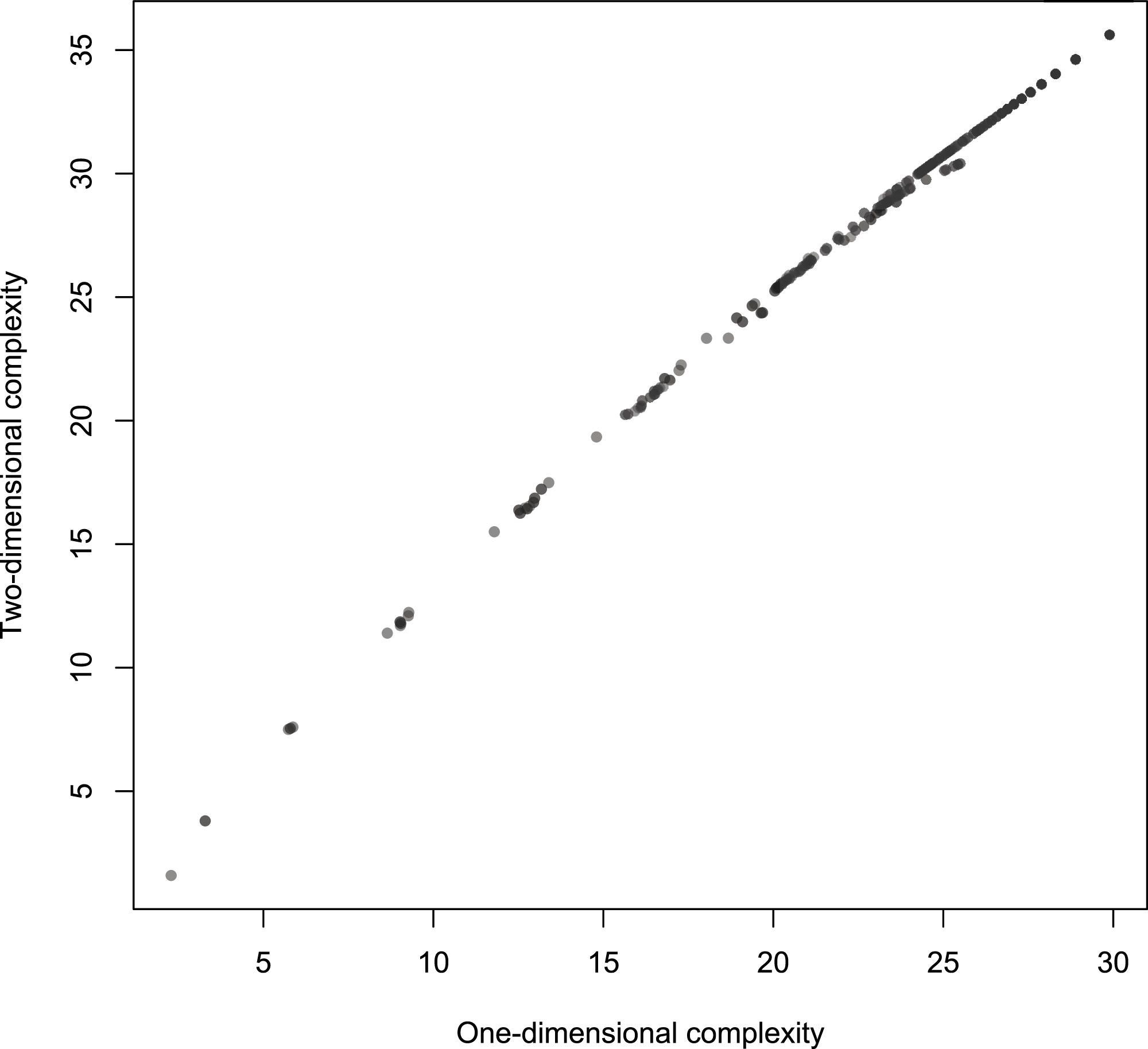
Figure 8: Scatterplot of Km with 2-dimensional Turing machines (Turmites) as a function of Km with 1-dimensional Turing machines.
All Turing machines in (4, 2) are included in (4, 2)2D because these are just the machines that do not move up or down. We first compared the values of the 1,832 output strings in (4, 2) to the 1-dimensional arrays found in (4, 2)2D. We are also interested in the relation between the ranks of these 1,832 strings in both (4, 2) and (4, 2)2D.

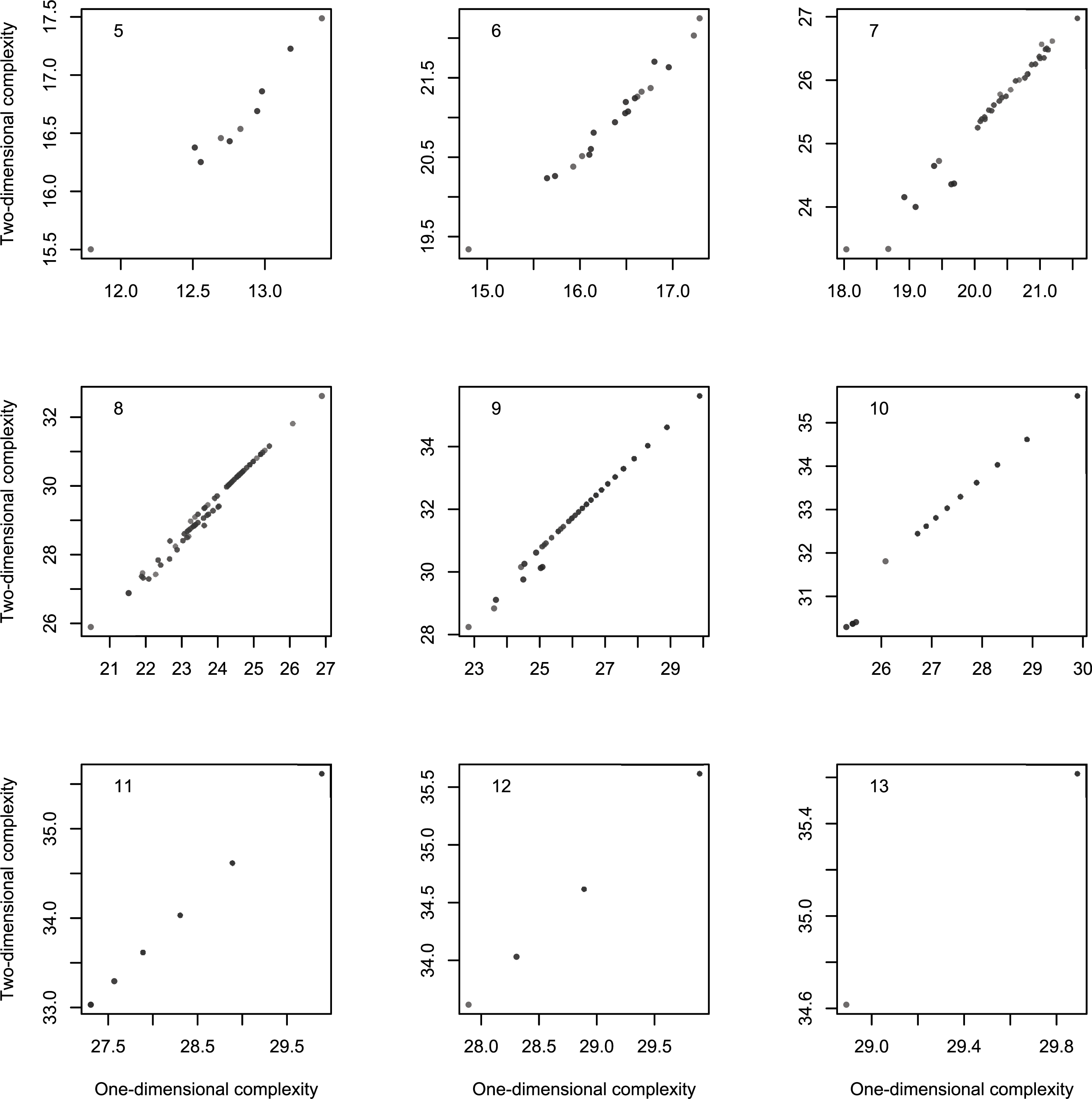
Figure 9: Scatterplot of Km with 2-dimensional Turing machines as a function of Km with 1-dimensional Turing machines by length of strings, for strings of length 5–13.
Figure 8 shows the link between Km,2D with 2D Turing machines as a function of ordinary Km,1D (that is, simply Km as defined in Soler-Toscano et al. (2014)). It suggests a strong almost-linear overall association. The correlation coefficient r = 0.9982 confirms the linear association, and the Spearman correlation coefficient rs = 0.9998 proves a tight and increasing functional relation.
The length l of strings is a possible confounding factor. However Fig. 9 suggests that the link between one and 2-dimensional complexities is not explainable by l. Indeed, the partial correlation rKm,1DKm,2D.l = 0.9936 still denotes a tight association.
Figure 9 also suggests that complexities are more strongly linked with longer strings. This is in fact the case, as Table 2 shows: the strength of the link increases with the length of the resulting strings. One and 2-dimensional complexities are remarkably correlated and may be considered two measures of the same underlying feature of the strings. How these measures vary is another matter. The regression of Km,2D on Km,1D gives the following approximate relation: Km,2D ≈ 2.64 + 1.11Km,1D. Note that this subtle departure from identity may be a consequence of a slight non-linearity, a feature visible in Fig. 8.
| Length (l) | Correlation |
|---|---|
| 5 | 0.9724 |
| 6 | 0.9863 |
| 7 | 0.9845 |
| 8 | 0.9944 |
| 9 | 0.9977 |
| 10 | 0.9952 |
| 11 | 1 |
| 12 | 1 |
Comparison of Km and compression of cellular automata
A 1-dimensional CA can be represented by an array of cells xi where i ∈ ℤ (integer set) and each x takes a value from a finite alphabet Σ. Thus, a sequence of cells {xi} of finite length n describes a string or global configuration c on Σ. This way, the set of finite configurations will be expressed as Σn. An evolution comprises a sequence of configurations {ci} produced by the mapping Φ:Σn → Σn; thus the global relation is symbolized as: (8) where t represents time and every global state of c is defined by a sequence of cell states. The global relation is determined over the cell states in configuration ct updated simultaneously at the next configuration ct+1 by a local function φ as follows: (9) Wolfram (2002) represents 1-dimensional cellular automata (CA) with two parameters (k, r) where k = |Σ| is the number of states, and r is the neighborhood radius. Hence this type of CA is defined by the parameters (2, 1). There are Σn different neighborhoods (where n = 2r + 1) and kkn distinct evolution rules. The evolutions of these cellular automata usually have periodic boundary conditions. Wolfram calls this type of CA Elementary Cellular Automata (denoted simply by ECA) and there are exactly kkn = 256 rules of this type. They are considered the most simple cellular automata (and among the simplest computing programs) capable of great behavioral richness.
1-dimensional ECA can be visualized in 2-dimensional space–time diagrams where every row is an evolution in time of the ECA rule. By their simplicity and because we have a good understanding about them (e.g., at least one ECA is known to be capable of Turing universality (Cook, 2004; Wolfram, 2002)) they are excellent candidates to test our measure Km,2D, being just as effective as other methods that approach ECA using compression algorithms (Zenil, 2010) that have yielded the results that Wolfram obtained heuristically.
Km,2D comparison with compressed ECA evolutions
We have seen that our Coding theorem method with associated measure Km (or Km,2D in this paper for 2D Kolmogorov complexity) is in agreement with bit string complexity as approached by compressibility, as we have reported in ‘Comparison of Km and approaches based on compression’.
The Universal Distribution from Turing machines that we have calculated (D(4, 2)2D) will help us to classify Elementary Cellular Automata. Classification of ECA by compressibility has been done before in Zenil (2010) with results that are in complete agreement with our intuition and knowledge of the complexity of certain ECA rules (and related to Wolfram’s (2002) classification). In Zenil (2010) both classifications by simplest initial condition and random initial condition were undertaken, leading to a stable compressibility classification of ECAs. Here we followed the same procedure for both simplest initial condition (single black cell) and random initial condition in order to compare the classification to the one that can be approximated by using D(4, 2)2D, as follows.
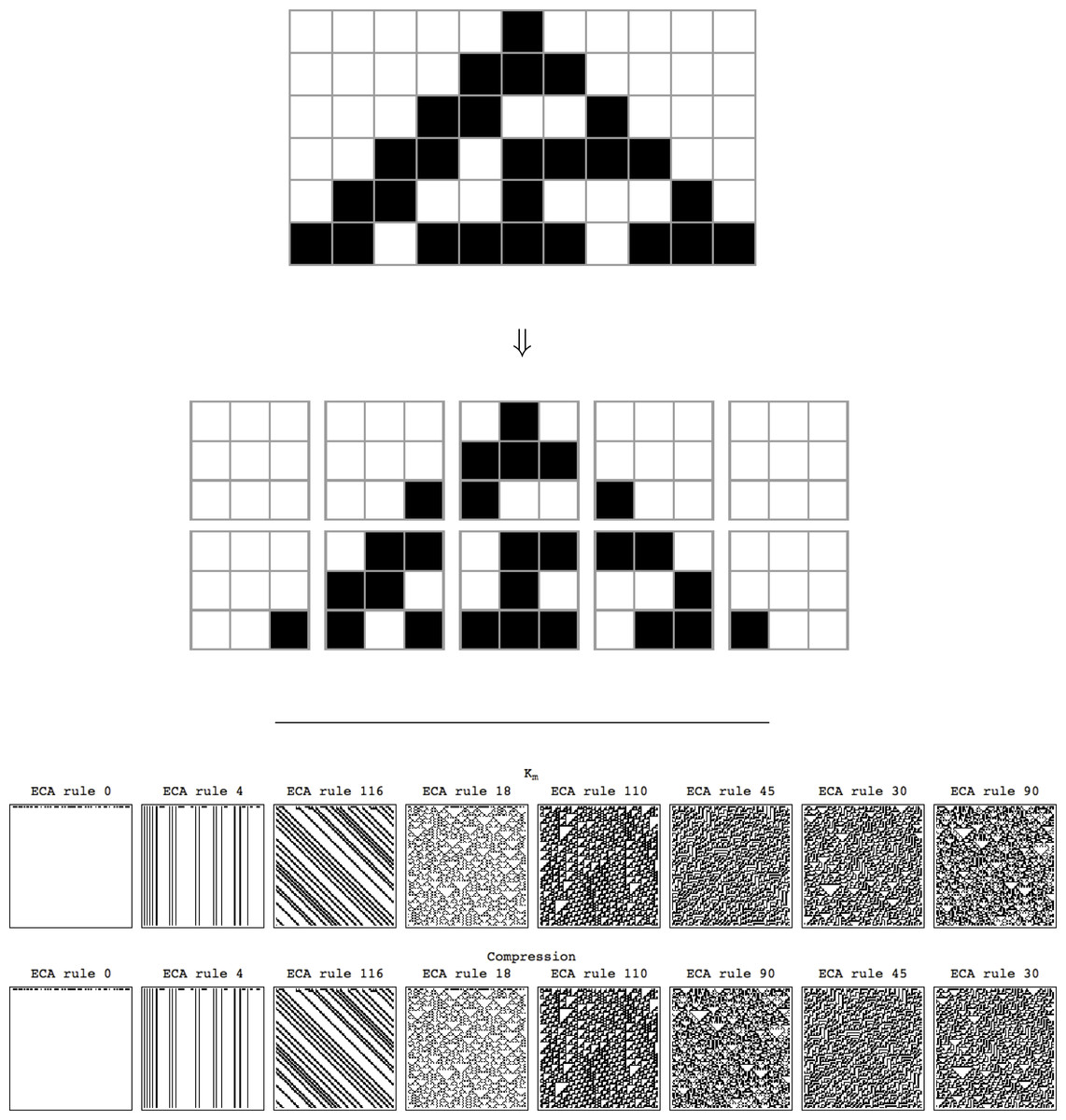
We will say that the space–time diagram (or evolution) of an Elementary Cellular Automaton c after time t has complexity: (10) That is, the complexity of a cellular automaton c is the sum of the complexities of the q arrays or image patches in the partition matrix {ct}d×d from breaking {ct} into square arrays of length d produced by the ECA after t steps. An example of a partition matrix of an ECA evolution is shown in Fig. 13 for ECA Rule 30 and d = 3 where t = 6. Notice that the boundary conditions for a partition matrix may require the addition of at most d − 1 empty rows or d − 1 empty columns to the boundary as shown in Fig. 13 (or alternatively the dismissal of at most d − 1 rows or d − 1 columns) if the dimensions (height and width) are not multiples of d, in this case d = 3.
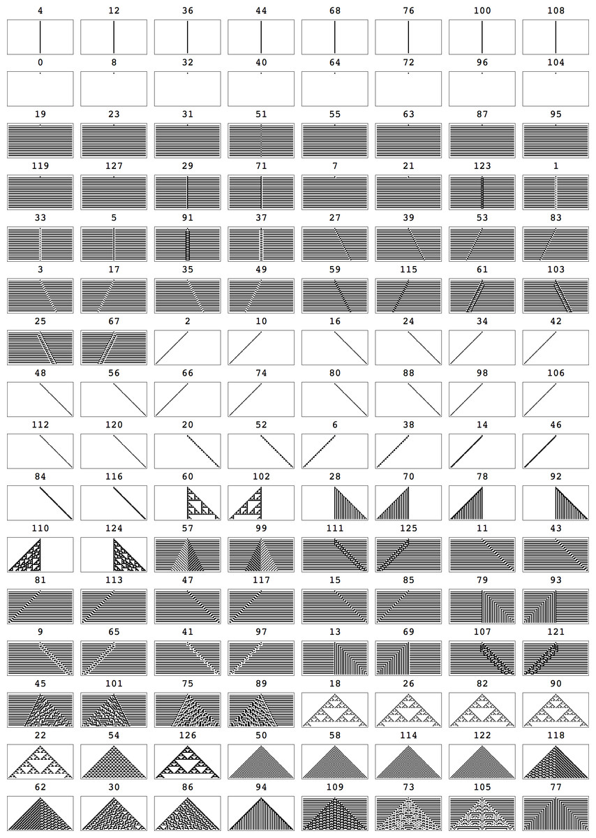
Figure 10: All the first 128 ECAs (the other 128 are 0–1 reverted rules) starting from the simplest (black cell) initial configuration running for t = 36 steps, sorted from lowest to highest complexity according to Km,2D3×3.
Notice that the same procedure can be extended for its use on arbitrary images.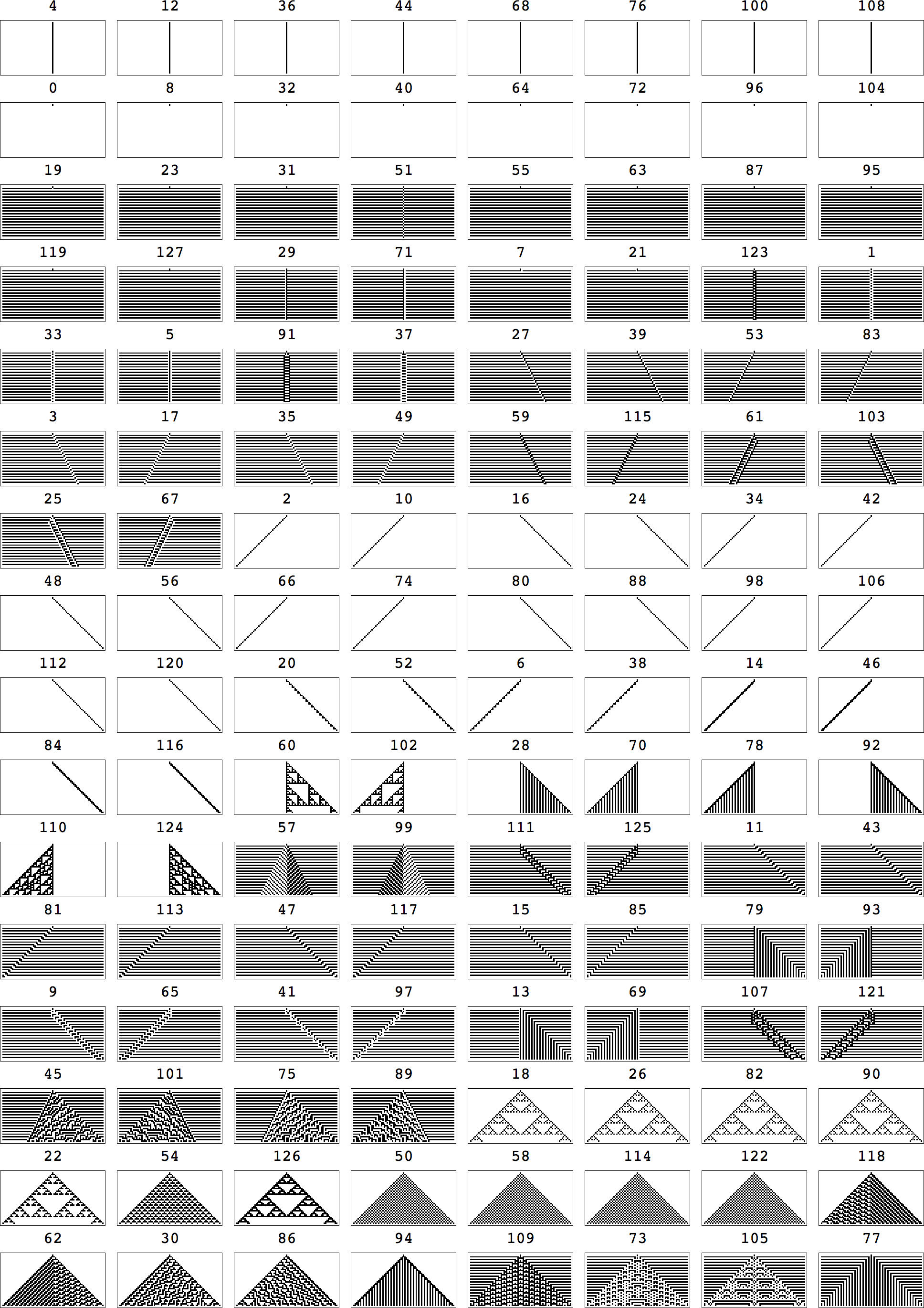
If the classification of all rules in ECA by Km,2D yields the same classification obtained by compressibility, one would be persuaded that Km,2D is a good alternative to compressibility as a method for approximating the Kolmogorov complexity of objects, with the signal advantage that Km,2D can be applied to very short strings and very short arrays such as images. Because all possible 29 arrays of size 3 × 3 are present in Km,2D we can use this arrays set to try to classify all ECAs by Kolmogorov complexity using the Coding Theorem method. Figure 6 shows all relevant (non-symmetric) arrays. We denote by Km,2D3×3 this subset from Km,2D.
Figure 11 displays the scatterplot of compression complexity against Km,2D3×3 calculated for every cellular automaton. It shows a positive link between the two measures. The Pearson correlation amounts to r = 0.8278, so the determination coefficient is r2 = 0.6853. These values correspond to a strong correlation, although smaller than the correlation between 1- and 2-dimensional complexities calculated in ‘Comparison of Km and approaches based on compression’.
Concerning orders arising from these measures of complexity, they too are strongly linked, with a Spearman correlation of rs = 0.9200. The scatterplots (Fig. 11) show a strong agreement between the Coding theorem method and the traditional compression method when both are used to classify ECAs by their approximation to Kolmogorov complexity.
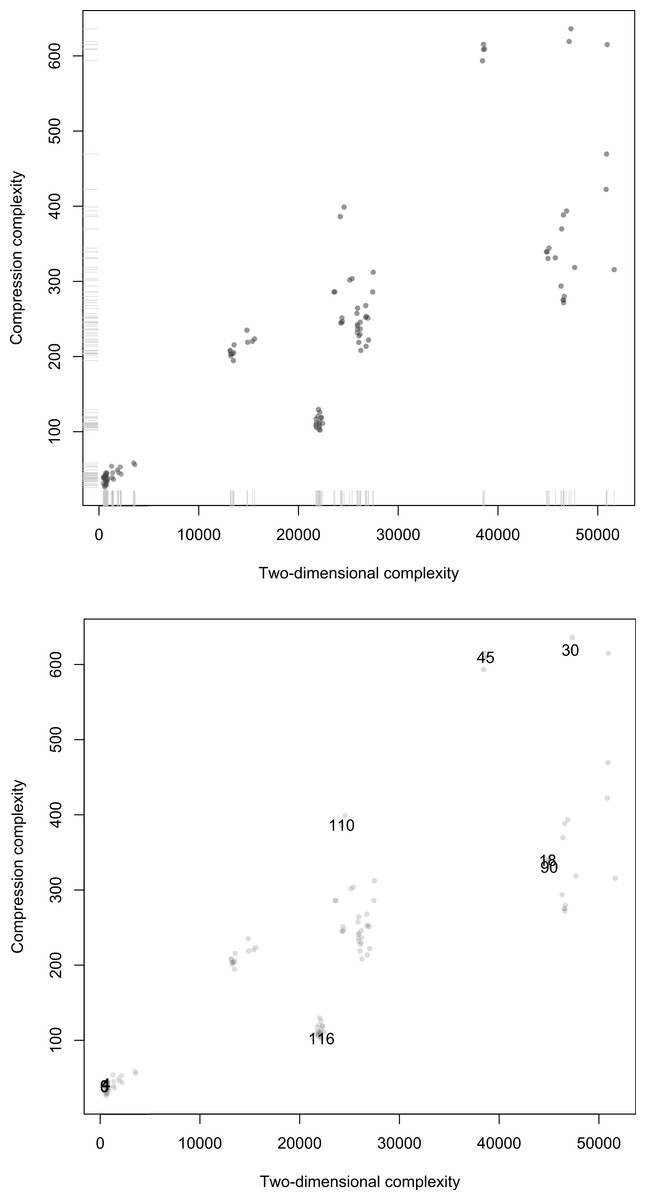
Figure 11: Scatterplots of Compress versus Km,2D3×3 on the 128 first ECA evolutions after t = 90 steps.
Top: Distribution of points along the axes displaying clusters of equivalent rules and a distribution corresponding to the known complexity of various cases. Bottom: Same plot but with some ECA rules highlighted some of which were used in the side by side comparison in Fig. 13 (but unlike there, here for a single black cell initial condition). That rules distribute on the diagonal indicates that both methods are correlated as theoretically expected (even if lossless compression is a form of entropy rate up to the compression fixed maximum word length).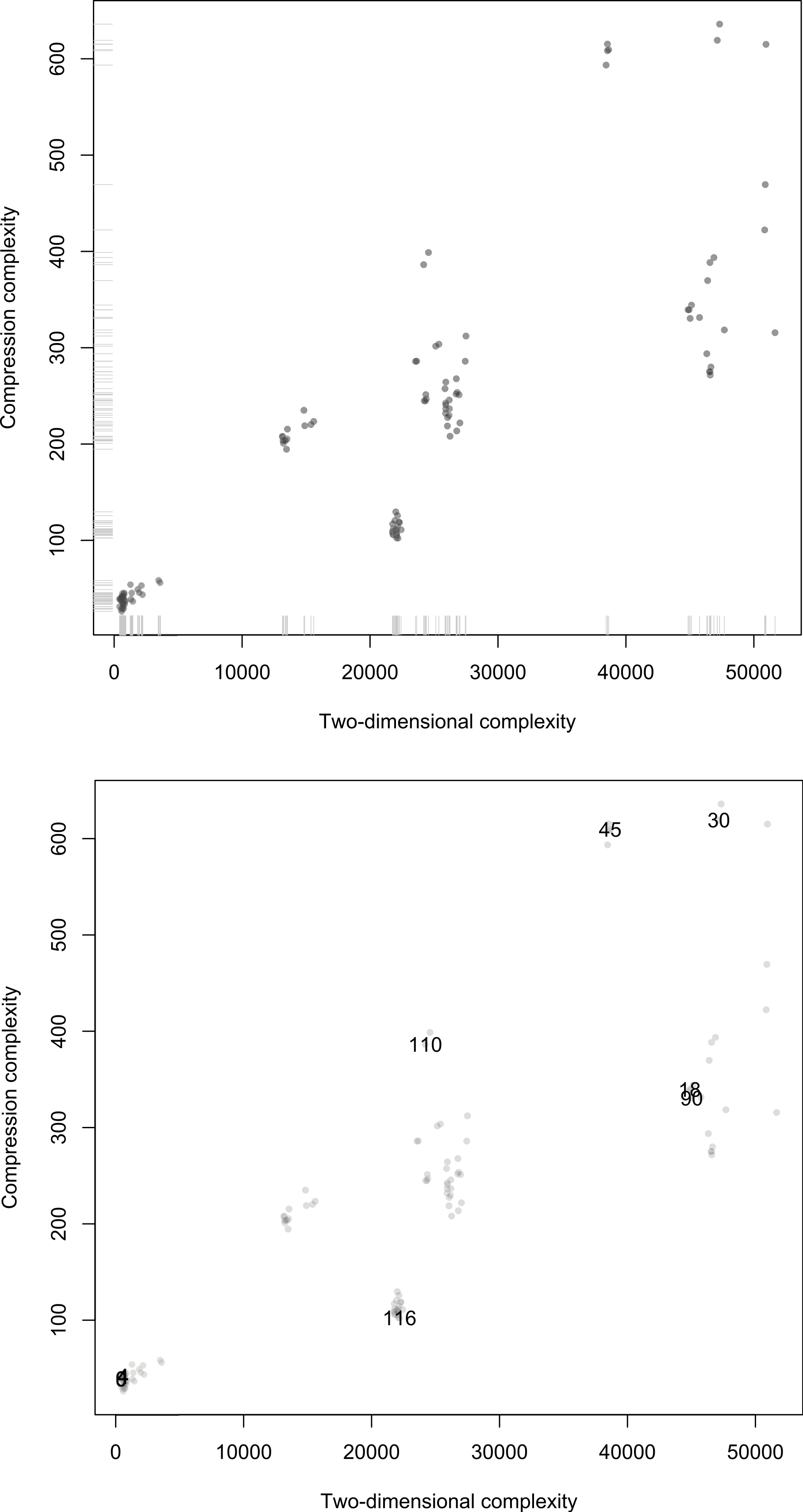
The anomalies found in the classification of Elementary Cellular Automata (e.g., Rule 77 being placed among ECA with high complexity according to Km,2D3×3) is a limitation of Km,2D3×3 itself and not of the Coding theorem method which for d = 3 is unable to “see” beyond 3-bit squares using, which is obviously very limited. And yet the degree of agreement with compressibility is surprising (as well as with intuition, as a glance at Fig. 10 shows, and as the distribution of ECAs starting from random initial conditions in Fig. 13 confirms). In fact an average ECA has a complexity of about 20K bits, which is quite a large program-size when compared to what we intuitively gauge to be the complexity of each ECA, which may suggest that they should have smaller programs. However, one can think of D(4, 2)2D3×3 as attempting to reconstruct the evolution of each ECA for the given number of steps with square arrays only 3 bits in size, the complexity of the three square arrays adding up to approximate Km,2D of the ECA rule. Hence it is the deployment of D(4, 2)2D3×3 that takes between 500 to 50K bits to reconstruct every ECA space–time evolution depending on how random versus how simple it is.
Other ways to exploit the data from D(4, 2)2D (e.g., non-square arrays) can be utilized to explore better classifications. We think that constructing a Universal Distribution from a larger set of Turing machines, e.g., D(5, 2)2D4×4 will deliver more accurate results but here we will also introduce a tweak to the definition of the complexity of the evolution of a cellular automaton.
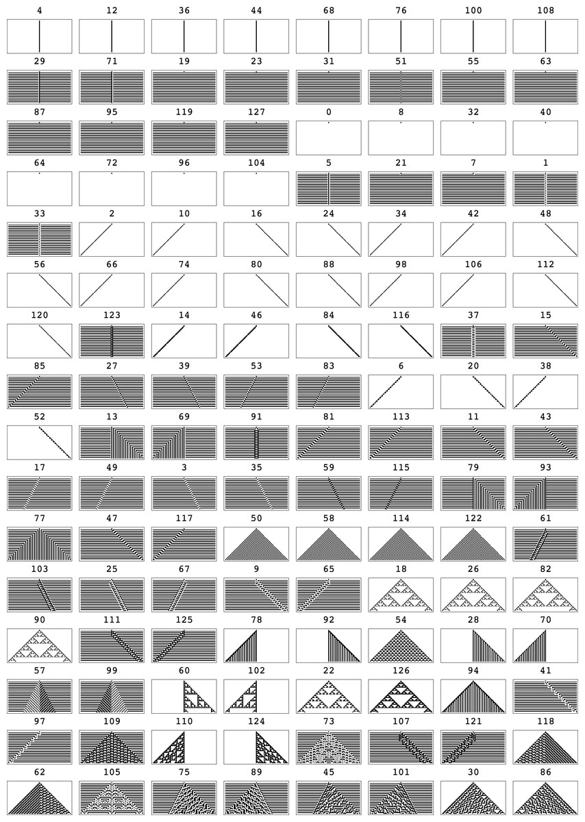
Figure 12: Block Decomposition Method.
All the first 128 ECAs (the other 128 are 0–1 reverted rules) starting from the simplest (black cell) initial configuration running for t = 36 steps, sorted from lowest to highest complexity according to Klog as defined in Eq. (11).
Splitting ECA rules in array squares of size 3 is like trying to look through little windows 9 pixels wide one at a time in order to recognize a face, or training a “microscope” on a planet in the sky. One can do better with the Coding theorem method by going further than we have in the calculation of a 2-dimensional Universal Distribution (e.g., calculating in full or a sample of D(5, 2)2D4×4), but eventually how far this process can be taken is dictated by the computational resources at hand. Nevertheless, one should use a telescope where telescopes are needed and a microscope where microscopes are needed.
Block Decomposition Method
One can think of an improvement in resolution of Km,2D(c) for growing space–time diagrams of cellular automaton by taking the log2(n) of the sum of the arrays where n is the number of repeated arrays, instead of simply adding the complexity of the image patches or arrays. That is, one penalizes repetition to improve the resolution of Km,2D for larger images as a sort of “optical lens”. This is possible because we know that the Kolmogorov complexity of repeated objects grows by log2(n), just as we explained with an example in ‘Kolmogorov–Chaitin Complexity’. Adding the complexity approximation of each array in the partition matrix of a space–time diagram of an ECA provides an upper bound on the ECA Kolmogorov complexity, as it shows that there is a program that generates the ECA evolution picture with the length equal to the sum of the programs generating all the sub-arrays (plus a small value corresponding to the code length to join the sub-arrays). So if a sub-array occurs n times we do not need to consider its complexity n times but log2(n). Taking into account this, Eq. (10) can be then rewritten as: (11) where ru are the different square arrays in the partition {ct}d×d of the matrix ct and nu the multiplicity of ru, that is the number of repetitions of d × d-length patches or square arrays found in ct. From now on we will use K′ for squares of size greater than 3 and it may be denoted only by K or by BDM standing for Block decomposition method. BDM has now been applied successfully to measure, for example, the Kolmogorov complexity of graphs and complex networks (Zenil et al., 2014) by way of their adjacency matrices (a 2D grid) and was shown to be consistent with labelled and unlabelled (up to isomorphisms) graphs.
Now complexity values of range between 70 and 3K bits with a mean program-size value of about 1K bits. The classification of ECA, according to Eq. (11), is presented in Fig. 12. There is an almost perfect agreement with a classification by lossless compression length (see Fig. 13) which makes even one wonder whether the Coding theorem method is actually providing more accurate approximations to Kolmogorov complexity than lossless compressibility for this objects length. Notice that the same procedure can be extended for its use on arbitrary images. We denominate this technique Block Decomposition Method. We think it will prove to be useful in various areas, including machine learning as an of Kolmogorov complexity (other contributions to ML inspired in Kolmogorov complexity can be found in Hutter (2003)).
Also worth notice that the fact that ECA can be successfully classified by Km,2D with an approximation of the Universal Distribution calculated from Turing machines (TM) suggests that output frequency distributions of ECA and TM cannot be but strongly correlated, something that we had found and reported before in Zenil & Delahaye (2010) and Delahaye & Zenil (2007b).
Another variation of the same Km,2D measure is to divide the original image into all possible square arrays of a given length rather than taking a partition. This would, however, be exponentially more expensive than the partition process alone, and given the results in Fig. 12 further variations do not seem to be needed, at least not for this case.
Robustness of the approximations to m(s)
One important question that arises when positing the soundness of the Coding theorem method as an alternative to having to pick a universal Turing machine to evaluate the Kolmogorov complexity K of an object, is how many arbitrary choices are made in the process of following one or another method and how important they are. One of the motivations of the Coding theorem method is to deal with the constant involved in the Invariance theorem (Eq. (2)), which depends on the (prefix-free) universal Turing machine chosen to measure K and which has such an impact on real-world applications involving short strings. While the constant involved remains, given that after application of the Coding theorem (Eq. (3)) we reintroduce the constant in the calculation of K, a legitimate question to ask is what difference it makes to follow the Coding theorem method compared to simply picking the universal Turing machine.
On the one hand, one has to bear in mind that no other method existed for approximating the Kolmogorov complexity of short strings. On the other hand, we have tried to minimize any arbitrary choice, from the formalism of the computing model to the informed runtime, when no Busy Beaver values are known and therefore sampling the space using an educated runtime cut-off is called for. When no Busy Beaver values are known the chosen runtime is determined according to the number of machines that we are ready to miss (e.g., less than .01%) for our sample to be significative enough as described in ‘Setting the runtime’. We have also shown in Soler-Toscano et al. (2014) that approximations to the Universal Distribution from spaces for which Busy Beaver values are known are in agreement with larger spaces for which Busy Beaver values are not known.
Among the possible arbitrary choices it is the enumeration that may perhaps be questioned, that is, calculating D(n) for increasing n (number of Turing machine states), hence by increasing size of computer programs (Turing machines). On the one hand, one way to avoid having to make a decision on the machines to consider when calculating a Universal Distribution is to cover all of them for a given number of n states and m symbols, which is what we have done (hence the enumeration in a thoroughly (n, m) space becomes irrelevant). While it may be an arbitrary choice to fix n and m, the formalisms we have followed guarantee that n-state m-symbol Turing machines are in (n + i, m + j) with i, j ≥ 0 (that is, the space of all n + i-state m + j-symbol Turing machines). Hence the process is incremental, taking larger spaces and constructing an average Universal Distribution. In fact, we have demonstrated (Soler-Toscano et al., 2014) that D(5) (that is, the Universal Distribution produced by the Turing machines with 2 symbols and 5 states) is strongly correlated to D(4) and represents an improvement in accuracy of the string complexity values in D(4), which in turn is in agreement with and an improvement on D(3) and so on. We have also estimated the constant c involved in the invariance theorem (Eq. (2)) between these D(n) for n > 2, which turned out to be very small in comparison to all the other calculated Universal Distributions (Soler-Toscano et al., 2013).
Real-world evidence
We have provided here some theoretical and statistical arguments to show the reliability, validity and generality of our measure, more empirical evidence has also been produced, in particular in the field of cognition and psychology where researchers often have to deal with too short strings or too small patterns for compression methods to be used. For instance, it was found that the complexity of a (one-dimensional) string better predicts its recall from short-term memory that the length of the string (Chekaf et al., 2015). Incidentally, a study on the conspiracy theory believers mindset also revealed that human perception of randomness is highly linked to our one-dimensional measure of complexity (Dieguez, Wagner-Egger & Gauvrit, 2015). Concerning the two-dimensional version introduced in this paper, it has been fruitfully used to show how language iterative learning triggers the emergence of linguistic structures (Kempe, Gauvrit & Forsyth, 2015). A direct link between the perception of two-dimensional randomness, our complexity measure, and natural statistics was also established in two experiments (Gauvrit, Soler-Toscano & Zenil, 2014). These findings further support the complexity metrics presented herein. Furthermore, more theoretical arguments have been advanced in Soler-Toscano et al. (2013) and Soler-Toscano & Zenil (2015).
Conclusions
We have shown how a highly symmetric but algorithmic process is capable of generating a full range of patterns of different structural complexity. We have introduced this technique as a natural and objective measure of complexity for n-dimensional objects. With two different experiments we have demonstrated that the measure is compatible with lossless compression estimations of Kolmogorov complexity, yielding similar results but providing an alternative particularly for short strings. We have also shown that Km,2D (and Km) are ready for applications, and that calculating Universal Distributions is a stable alternative to compression and a potential useful tool for approximating the Kolmogorov complexity of objects, strings and images (arrays). We think this method will prove to do the same for a wide range of areas where compression is not an option given the size of strings involved.
We also introduced the Block Decomposition Method. As we have seen with anomalies in the classification such as ECA Rule 77 (see Fig. 10), when approaching the complexity of the space–time diagrams of ECA by splitting them in square arrays of size 3, the Coding theorem method does have its limitations, especially because it is computationally very expensive (although the most expensive part needs to be done only once—that is, producing an approximation of the Universal Distribution). Like other high precision instruments for examining the tiniest objects in our world, measuring the smallest complexities is very expensive, just as the compression method can also be very expensive for large amounts of data.
We have shown that the method is stable in the face of the changes in Turing machine formalism that we have undertaken (in this case Turmites) as compared to, for example, traditional 1-dimensional Turing machines or to strict integer value program-size complexity (Soler-Toscano et al., 2013) as a way to estimate the error of the numerical estimations of Kolmogorov complexity through algorithmic probability. For the Turing machine model we have now changed the number of states, the number of symbols and now even the movement of the head and its support (grid versus tape). We have shown and reported here and in Soler-Toscano et al. (2014) and Soler-Toscano et al. (2013) that all these changes yield distributions that are strongly correlated with each other up to the point to assert that all these parameters have marginal impact in the final distributions suggesting a fast rate of convergence in values that reduce the concern of the constant involved in the invariance theorem. In Zenil & Delahaye (2010) we also proposed a way to compare approximations to the Universal Distribution by completely different computational models (e.g., Post tag systems and cellular automata), showing that for the studied cases reasonable estimations with different degrees of correlations were produced. The fact that we classify Elementary Cellular Automata (ECA) as shown in this paper, with the output distribution of Turmites with results that fully agree with lossless compressibility, can be seen as evidence of agreement in the face of a radical change of computational model that preserves the apparent order and randomness of Turmites in ECA and of ECA in Turmites, which in turn are in full agreement with 1-dimensional Turing machines and with lossless compressibility.
We have made available to the community this “microscope” to look at the space of bit strings and other objects in the form of the Online Algorithmic Complexity Calculator (http://www.complexitycalculator.com) implementing Km (in the future it will also implement Km,2D and many other objects and a wider range of methods) that provides objective algorithmic probability and Kolmogorov complexity estimations for short binary strings using the method described herein. Raw data and the computer programs to reproduce the results for this paper can also be found under the Publications section of the Algorithmic Nature Group (http://www.algorithmicnature.org).
Supplemental Information
Supplemental material with necessary data to validate results
Contents: CSV files and output distribution of all 2D TMs used by BDM to calculate the complexity of all arrays of size 3 × 3 and ECAs.