A Rigid Motion Artifact Reduction Method for CT Based on Blind Deconvolution

1
School of Electrical and Information Engineering, Tianjin University, Tianjin 300072, China
2
School of Information Engineering, Tianjin University of Commerce, Tianjin 300134, China
*
Author to whom correspondence should be addressed.
Algorithms 2019, 12(8), 155; https://0-doi-org.brum.beds.ac.uk/10.3390/a12080155
Submission received: 15 July 2019
/
Accepted: 29 July 2019
/
Published: 31 July 2019
(This article belongs to the Special Issue The Second Symposium on Machine Intelligence and Data Analytics)
Abstract
:In computed tomography (CT), artifacts due to patient rigid motion often significantly degrade image quality. This paper suggests a method based on iterative blind deconvolution to eliminate motion artifacts. The proposed method alternately reconstructs the image and reduces motion artifacts in an iterative scheme until the difference measure between two successive iterations is smaller than a threshold. In this iterative process, Richardson–Lucy (RL) deconvolution with spatially adaptive total variation (SATV) regularization is inserted into the iterative process of the ordered subsets expectation maximization (OSEM) reconstruction algorithm. The proposed method is evaluated on a numerical phantom, a head phantom, and patient scan. The reconstructed images indicate that the proposed method can reduce motion artifacts and provide high-quality images. Quantitative evaluations also show the proposed method yielded an appreciable improvement on all metrics, reducing root-mean-square error (RMSE) by about 30% and increasing Pearson correlation coefficient (CC) and mean structural similarity (MSSIM) by about 15% and 20%, respectively, compared to the RL-OSEM method. Furthermore, the proposed method only needs measured raw data and no additional measurements are needed. Compared with the previous work, it can be applied to any scanning mode and can realize six degrees of freedom motion artifact reduction, so the artifact reduction effect is better in clinical experiments.
1. Introduction
As one of the important technologies in medical diagnosis, a CT image can achieve a high performance in detecting and measuring small lesions [1,2]. However, CT has a problem that the reconstructed image will suffer from motion artifacts if a moving object is reconstructed without motion correction, in severe cases resulting in false diagnosis [3]. To reduce motion artifacts, the main approaches are shortening the scan time [4,5], external motion monitoring techniques [6,7,8], and motion estimation and compensation methods [9]. Since the third category of methods has the advantages of neither increasing hardware cost or design difficulty nor requiring additional devices, it has been widely studied. Among these methods, some were intended for 2D parallel-beam or fan-beam geometries and needed to assume a motion model that is an approximation of the real motion [9,10,11]. In [9], a novel method based on the Helgason-Ludwig consistency condition (HLCC) for estimation of rigid motion in fan-beam geometry was presented. Once the motion has been estimated, a compensation for the motion can be performed. This method has the disadvantages of large computational complexity and poor estimation accuracy. To solve this problem, a new method based on frequency domain analysis was proposed [10]. Motion parameters can be determined by the magnitude correlation of projections in frequency domain. This method was more accurate and faster on the performance of motion estimation than the method based on the HLCC. Using this method, a new method based on extended difference function was proposed, which further reduced the complexity of computation [11]. However, these three methods can only achieve in-plane motion estimation, which has limitations in clinical application. Some addressed the problem for cone beam CT (CBCT), but only for CBCT [12,13]. Other methods iteratively estimated and compensated the motion during the reconstruction for head CT when head motion occurs in all six degrees of freedom (d.o.f.). Sun et al. devised an iterative motion estimation and compensation scheme for helical CT [14]. Jang et al. proposed a motion estimation and compensation method based on filtered back projection for CBCT [15]. Chen et al. presented a motion artifact correction method based on local linear embedding for CBCT [16]. However, these methods cannot always estimate the motion parameters accurately, since the pose of the reconstructed object is arbitrary and slow components of the motions may not be fully estimated. Therefore, the goal of this paper is to develop a motion artifact reduction method that does not need to estimate the motion and can be suitable for any scanning mode.
The aim of blind deconvolution (BD) is to recover an image without complete knowledge of the associated system function, which has been widely applied in medical images to improve the quality of images [17]. However, the deconvolution does not converge to the solution because the noise is amplified after iterations [18,19,20]. With the purpose of avoiding degradation of the image quality, recent works use the spatially adaptive total variation (SATV) as a regularization term [21].
A motion-blurred CT image can be considered as a convolution of a degraded system and original image. Therefore, the true image can be estimated from the blurred image using iterative blind deconvolution. The reason for selecting the image domain over the sinogram domain is because motion effects are better understood and motion trajectories are more tractable to model in the image space. In fact, motion artifacts are mainly manifested in strip artifacts, blurred tissue images, displacement of image contours and objects with similar attachments in the cavity. Thus, this paper develops a motion artifact reduction approach based on iterative blind deconvolution for CT image. The rigid motion is characterized by six d.o.f. (three rotations and three translations) [7]. The proposed method bring Richardson–Lucy (RL) deconvolution with SATV regularization into the ordered subset expectation maximization (OSEM) iteration. Since the OSEM is a fast iterative algorithm, which has the advantages of good spatial resolution, strong anti-noise ability, and fast reconstruction speed, it is widely used in CT image reconstruction. Thus, this paper chooses this algorithm for image reconstruction. In the iteration process, image reconstruction and motion artifact reduction are completed. The iterations are stopped when the difference measure between two successive iterations is smaller than a threshold. The proposed method does not have to estimate the motion and is not limited by scanning mode. The efficacy of the proposed method is demonstrated on a modified 3D Shepp–Logan phantom, a head phantom and patient scan. The simulation results show that the proposed method can reduce RMSE by about 30% more than the RL-OSEM method, and increase CC and MSSIM by about 15% and 20% more than the RL-OSEM method.
The contribution of this paper is given as follows:
- Richardson–Lucy (RL) deconvolution with SATV regularization is brought into the ordered subset expectation maximization (OSEM) iteration.
- With the proposed method, image reconstruction and motion artifact reduction are completed alternately in the iteration process.
- The simulation results are given to verify that the proposed method can be applied to any scanning mode.
2. Methods
2.1. Ordered Subset Expectation Maximization (OSEM) Reconstruction
In order to correct the motion during the reconstruction, an iterative reconstruction algorithm is needed. OSEM is used as the reconstruction algorithm [14,22].
where is the estimated activity in voxel j after iteration n, is the measured sinogram, is the system matrix element representing the probability that a photon emitted from voxel j is detected in detector pixel i, and is one subset.
2.2. Iterative Blind Deconvolution
2.2.1. Image Degradation Model
The generation of CT images can be modeled as an image degradation system. The motion-degraded image is formed by a convolution between the ideal image and the point spread function (PSF) [23].
where is the degraded image, is the ideal image, is the impulse response of the system or PSF, s denotes the spatial coordinates, and ∗ is the convolution in spatial domain.
In practice, the PSF is not precisely known. Hence, an iterative blind deconvolution approach is needed to restore the real image without complete knowledge of the associated system PSF.
2.2.2. RL Deconvolution with SATV Regularization
RL can effectively solve nuclear medical imaging problems, which is derived from the maximum likelihood of a Poisson distribution. The TV model was first proposed by Rudin et al. [24] in edge preserving image restoration, it is a popular choice of being the regularization term [25]. RL algorithm with total variation regularization (RLTV) was suggested in [26,27].
where is the regularization parameter, refers to divergence, represents l2-norm, and denotes the gradient operator.
In Equation (4), plays a very important role, which controls the TV regularization strength. It should be neither too small nor too large: if is too small, the noise will not be well suppressed; inversely, if it is too large, the edge and detailed information in image will be blurred. Therefore, a spatially adaptive TV regularization model considering the spatial dependent property is introduced [21,28].
the term in the denominator provide an estimate of edges from an initial image f0 at scale using the Gaussian kernel filtered gradients, and ε is a parameter of adaptive function . The spatially adaptive function can help reduce noise without producing the staircase effect because it can self-adjust according to the smoothed gradient of the image. To summarize, the SATV regularization has two good features: (1) For edge and detail, because is small which weakens the TV regularization, then the edge and texture will be well preserved; (2) for flat region, a large leads to a large TV regularization strength, so the noise will be well suppressed.
2.3. Motion Artifact Reduction in Reconstruction
To reduce motion artifacts, iterative blind deconvolution algorithm is inserted into the iterative process of OSEM reconstruction. Hence, Equation (1) can be modified as
In Equation (6), it is assumed that the estimation of degraded image () is still a Poisson distribution. The corresponding projection of estimated motion-degraded image are compared with the measured projection data to estimate the ideal image and PSF. The overall process of the BD-OSEM method is shown in Figure 1.
As shown in Figure 1, px represents input image size. The result of each OSEM-iteration is used as the degraded image for the BD-iteration (), while the result of the BD-iteration is returned to the OSEM-iteration as intermediate value for the next iteration. To stop the iterations, a difference measure between two successive iterations is defined [29]. If the difference is smaller than a threshold, the computation is stopped, and the last estimation is the best one. The criterion is defined as the following:
In Figure 1, if , the result of the BD-iteration will be returned to the next BD-iteration. If and , the result of the BD-iteration will be inserted to the iteration of OSEM, which is used as intermediate value. Note that the process of BD-OSEM is stopped at two or more iterations; hence, and should be satisfied.
3. Results
3.1. Numerical Phantom Experiments
For the numerical simulations, the modified three-dimensional version of the Shepp–Logan phantom was used to simulate the CBCT system. The additional tiny circles in the 128th slice of modified 3D Shepp–Logan head phantom are used to simulate the small tissue, as shown in Figure 2a. The size of the phantom was 256 × 256 × 256 voxels and the display window was [0 HU, 1000 HU]. The scanning time was set to . The interval angle was 1°, and the number of projections was 360. The distance from X-ray source to detector was 100 cm and source to object was 50 cm. Poisson noise was added to the raw simulated data before the reconstruction (assuming that 10,000 photons were detected on each detector element in the blank scan).
The projection data were obtained by applying the motion to a phantom during the scan. Figure 3 shows the motion segment that was used in the simulations. The slight motion of up 4° and 7 mm for rotations and translations obtained by Kim et al. [7] (a motion segment in Figure 15 of [7]) are presented in Figure 3a. Figure 3b shows the large motion exceeding 30° and 30 mm, which is much larger than that typically expected in patients [7].
In simulations, a parameter and the smoothness parameter were used for computations and the iterations were stopped when the difference between two images is less than a chosen threshold . For the OSEM reconstruction, four iterations with 60 subsets were applied. The deconvolution were stopped at the third iteration for the BD-iteration.
Figure 4 shows the 128th slice of reconstructed images obtained by four methods. In this paper, “OSEM-BD” refers the method based on OSEM reconstruction algorithm with motion correction by BD-iteration, and “RL-OSEM” represents the method based on the combination of RL deconvolution and OSEM reconstruction, that is the proposed method without SATV regularization. It can be seen that the motion-corrected image obtained by the proposed method is very close to the real phantom. Since the motion information is constantly superimposed in the reconstruction process, the OSEM-BD method cannot completely eliminate the motion artifacts. In addition, the RL-OSEM method cannot balance edge preservation and noise amplification very well because it has no regularization constraints, so there are some motion artifacts and intensity oscillations in the reconstructed image. The proposed method can overcome the problems of RL-OSEM method. Thus, the reconstructed image obtained by the proposed method is the clearest and most of the motion artifacts are eliminated.
The effects of motion artifact reduction were evaluated by visual assessment and with quantitative analysis. The root-mean-square error (RMSE), Pearson correlation coefficient (CC), and mean structural similarity (MSSIM) were chose as the metrics. RMSE was calculated in HU, while CC and MSSIM were dimensionless [7]. Table 1 provides quantitative comparisons of all reconstructed images among four methods. The mean and standard deviation of each metric were calculated over 256 reconstructed slices. The means (RMSE, CC, and MSSIM) indicated the overall quality of the reconstructed images. Standard deviations were taken as indices of the slice-to-slice variation in the calculated metrics. As expected, images reconstructed by using the proposed algorithm provide much higher CC and MSSIM mean values and much lower RMSE mean values. All the standard deviations of the proposed method are much lower than the other three methods, which demonstrate the proposed method has better stability. The simulation results of slight motion show that the proposed method has better motion artifact reduction effect than OSEM-BD and RL-OSEM method.
To further evaluate the proposed method, the projection data were obtained by applying a large motion. Figure 5 shows the 128th slice of images reconstructed from projection with large motion. The metric values for four different methods are shown in Table 2. Three metrics of the proposed method are better than the other three methods. Nevertheless, the motion-corrected image obtained by the proposed method still has residual artifacts. Because the reconstructed image is badly damaged and motion artifacts are very serious, it cannot be corrected by the proposed method. The simulation results of large motion show that the proposed method has a poor motion artifact reduction effect, but it is still better than OSEM-BD and RL-OSEM methods.
3.2. Head Phantom Experiments
In the following simulations, the proposed method was verified on head phantom. A selected slice of head phantom was shown in Figure 2b. The sinogram was acquired from head phantom with motion and noise that were the same as the Shepp–Logan phantom experiments. The head CT image was acquired from a GE Hi-Speed multi-slice CT scanner. A total of 720 views were uniformly selected over a 360° range under 150 mA X-ray tube current and 120 kVp. The display window was [−5 HU, 75 HU]. All of the reconstructed images (512 × 512 pixels) were reconstructed by the OSEM method with three iterations and 30 subsets. BD-iterations were stopped at the sixth iteration. The other experimental parameters were set the same as those of the Shepp–Logan phantom experiments.
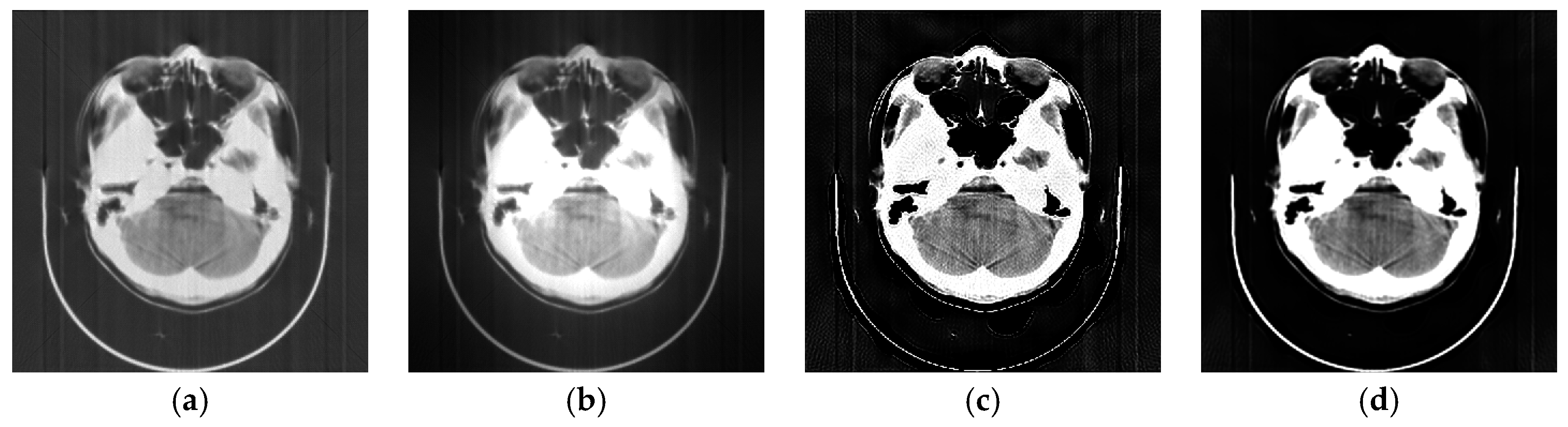
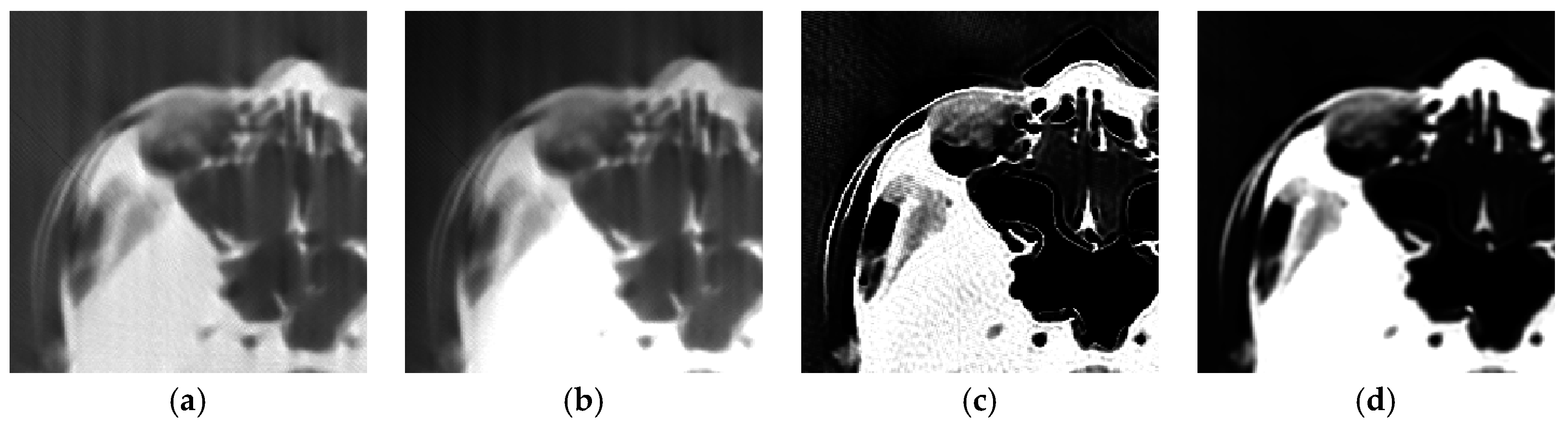
Figure 6 shows the selected slice of reconstructed images obtained by using OSEM, OSEM-BD, RL-OSEM, and the proposed method. To view the texture of reconstructed images more clearly, the zoomed images of a region of interest (ROI) from the corresponding images of Figure 6 are shown in Figure 7. Clearly, the proposed method is superior to the other methods in image quality.
To quantitatively evaluate the proposed method for head phantom, all slices of reconstructed images were compared by RMSE, CC, and MSSIM, as shown in Table 3. Clearly, the proposed method provides the highest CC and MSSIM mean values and the lowest RMSE mean values. All the standard deviations of the proposed method are much lower than the other three methods. The results indicate that the proposed method has a better performance on motion artifact reduction.
3.3. Patient Scan Experiments
To verify the effectiveness of the proposed method on the clinical data with realistic motion, the method was applied to clinical experiments in which motion artifacts had been observed. The scan was performed on a GE Light Speed VCT scanner. The scan parameters were tube voltage 120 kVp and tube current 200 mA. Image size was 512 × 512 pixels and the display window was [−5 HU, 75 HU]. Because the patient bed did not move with the patient during the scan, the patient bed data were removed. Three iterations with 30 subsets were applied for OSEM reconstruction, and four iterations for the BD-iteration. The other experimental parameters were set the same as those of the Shepp–Logan phantom experiments.
Figure 8 shows the selected slice of reconstructed images and the repeated scan image (which is done because of the observed motion in the first scan). The uncorrected image was reconstructed with the scanner system software, as shown in Figure 8a. Table 4 shows the comparisons of RMSE, CC and MSSIM. Note that all reconstructed images were registered to the repeated scan before the calculation of these metrics. Because the positional differences are irrelevant for image quality [14,30]. The results of patient scan experiments show that the reconstructed image obtained by the proposed method can effectively eliminate motion artifacts, and the artifact reduction effect of the proposed method is better than OSEM-BD and RL-OSEM methods.
4. Discussion
The performance of the proposed method was verified by using a modified 3D Shepp–Logan phantom, a head phantom, and patient scan. In numerical phantom experiments, the proposed method produced higher quality images for the case of slight motion than the other three considered approaches. As illustrated in Figure 4a,b, the images included severe motion artifacts over the whole image, and thereby inner structures and the skull were noticeably distorted. In Figure 4c,d the majority of distortions were eliminated. But many intensity oscillations appeared inside the phantom (see Figure 4c). The proposed method yielded an appreciable improvement on all metrics, reducing RMSE by about 30% and increasing CC and MSSIM by about 14% and 19%, respectively, compared to the RL-OSEM method (see Table 1). However, the proposed method did not perform well in cases of large motion, such as that of Figure 3b. Since the OSEM reconstruction was corrupted severely, these motion artifacts were too severe to be corrected by the proposed method (see Figure 5d). Therefore, a limitation of the method is that the proposed method usually did not perform well when the amplitude of the rotations was more than 30° and the amplitude of the translations was more than 30 mm.
In head phantom experiments, the reconstructed images showed marked improvement when the proposed method was applied. As shown in Figure 6a,b the reconstructed images exhibited severe motion artifacts and distorted image quality. And the image reconstructed by the RL-OSEM method still had artifacts and its edge appeared thinner than the true image (see Figure 6c and Figure 7c). All the metrics also suggested improvement motion correction performance on the proposed method. The RMSE of the proposed method was the smallest and reduced by about 27% compared to the RL-OSEM method; the CC and MSSIM of the proposed method were the greatest and increased by about 15% and 20%, respectively, compared to the RL-OSEM method (see Table 3).
Comparative results on numerical phantom and head phantom show that the OSEM-BD method can eliminate noise but not reduce motion artifacts. The BD-OSEM method can effectively reduce motion artifacts and the noise in flat regions as well as preserve the edge and detailed information.
In patient scan experiments, the reconstructed images, even with motion correction, provided severe motion artifacts (see Figure 8b,c). Most of the motion artifacts in the reconstructed image were eliminated after the motion correction by the proposed method (see Figure 8d). The RMSE of the proposed method can reduce by about 30%, compared to the RL-OSEM method; the CC and MSSIM of the proposed method can increase by about 15% and 21%, respectively, compared to the RL-OSEM method (see Table 4).
The computation will take a long time since there are a large number of CT views in clinical scans. Currently, the computation complexity of the proposed method is mainly the OSEM reconstruction for a patient scan, which improves the computation efficiency compared to the method mentioned in [14] to some extent.
The performance of the proposed method has been verified by using a patient scan. However, this experiment may not be sufficient to demonstrate the algorithm for various clinical cases. In the future, more clinical experiments should be considered.
5. Conclusions
In this work, a method based on iterative blind deconvolution is developed to reduce the rigid motion artifacts for CT, which only requires the measured raw data. Since the OSEM is a fast iterative algorithm and widely used in CT image reconstruction, this paper uses OSEM as the reconstruction algorithm. As well as, RL iteration algorithm can estimate a clear image only based on original data and SATV regularization can effectively preserve image edge and detail information, while removing noise effects, so this paper uses RL algorithm with SATV regularization (RLSATV) to eliminate motion artifacts. Therefore, this paper combines the OSEM algorithm with RLSATV to complete image reconstruction and motion artifact reduction in the iteration process. In the process of iteration, the RL algorithm which is regularized using SATV is inserted into the iterative process of the OSEM reconstruction technique. The iteration process does not end until the difference measure between two successive iterations is smaller than a threshold. The proposed method has been evaluated by using phantom and patient scan experiments, which can reduce motion artifacts and provide high-quality images. Quantitative analysis results show that the RMSE of the proposed method can reduce by about 30% compared to the RL-OSEM method; the CC and MSSIM of the proposed method can increase by about 15% and 20%, respectively, compared to the RL-OSEM method. Additionally, the proposed method does not have to estimate the motion and is suitable for any scanning mode, thus it can become a valuable tool for motion compensation in clinical application.
Author Contributions
Y.Z. contributed to the overall idea of the algorithms, carried out the simulations, and drafted the manuscript; L.Z. supervised the work and provided the major direction of the research. All authors have read and approved the final manuscript.
Funding
This research was funded by National Natural Science Foundation of China, grant number 61340034, China Postdoctoral Science Foundation, grant number 2013M530873, Tianjin Research Program of Application Foundation and Advanced Technology, grant number 13JCYBJC15600, Natural Science Foundation of Tianjin of China, grant number 16JCYBJC28800. The APC was funded by 16JCYBJC28800.
Acknowledgments
This work was supported by National Natural Science Foundation of China (No.61340034), China Postdoctoral Science Foundation (No.2013M530873), Tianjin Research Program of Application Foundation and Advanced Technology (No.13JCYBJC15600), Natural Science Foundation of Tianjin of China (No. 16JCYBJC28800). We are grateful to the anonymous reviewers whose comments and suggestions have contributed to improving the quality of research that is described in this paper.
Conflicts of Interest
The authors declare no conflicts of interest.
Abbreviations
| BD | Blind Deconvolution |
| BD-OSEM | the combination of Blind Deconvolution and Ordered Subset Expectation Maximization reconstruction |
| CC | Pearson Correlation Coefficient |
| CT | Computed Tomography |
| CBCT | Cone Beam CT |
| HLCC | Helgason-Ludwig Consistency Condition |
| MSSIM | Mean Structural Similarity |
| OSEM | Ordered Subsets Expectation Maximization |
| OSEM-BD | OSEM reconstruction algorithm with motion correction by BD-iteration |
| PSF | Point Spread Function |
| RL | Richardson–Lucy |
| RL-OSEM | the combination of Richardson–Lucy deconvolution and OSEM reconstruction |
| RMSE | Root-Mean-Square Error |
| RLTV | RL Algorithm with Total Variation Regularization |
| RLSATV | RL algorithm with SATV regularization |
| ROI | Region of Interest |
| SATV | Spatially Adaptive Total Variation |
References
- Kim, J.H.; Sun, T.; Alcheikh, A.R.; Kuncic, Z.; Nuyts, J.; Fulton, R. Correction for human head motion in helical X-ray CT. Phys. Med. Biol. 2016, 61, 1416–1438. [Google Scholar] [CrossRef] [PubMed]
- Liu, J.; Ma, J.; Zhang, Y.; Chen, Y.; Yang, J.; Shu, H.; Luo, L.; Goatrieux, G.; Yang, W.; Feng, Q.; et al. Discriminative feature representation to improve projection data inconsistency for low dose CT imaging. IEEE Trans. Med. Imaging 2018, 36, 2499–2509. [Google Scholar] [CrossRef] [PubMed]
- Chen, Y.; Zhang, Y.; Yang, J.; Shu, H.; Luo, L.; Coatrieux, J.L.; Feng, Q. Structure-adaptive fuzzy estimation for random-valued impulse noise suppression. IEEE Trans. Circuits Syst. Video Technol. 2018, 28, 414–427. [Google Scholar] [CrossRef]
- Fahmi, F.; Henk, A.M.; Geert, J.S.; Ludo, F.M.B.; Natasja, N.Y.J.; Charles, B.L.M.; Ed, B. Automatic detection of CT perfusion datasets unsuitable for analysis due to head movement of acute ischemic stroke patients. J. Healthc. Eng. 2014, 5, 67–78. [Google Scholar] [CrossRef] [PubMed]
- Li, L.; Chen, Z.; Jin, X.; Yu, H.; Wang, G. Experimental measurement of human head motion for high-resolution computed tomography system design. Opt. Eng. 2010, 49, 063201. [Google Scholar] [CrossRef]
- Chandler, A.; Wei, W.; Herron, D.H. Semiautomated motion correction of tumors in lung CT-perfusion studies. Acad. Radiol. 2011, 18, 286–293. [Google Scholar] [CrossRef]
- Kim, J.H.; Nuyts, J.; Kyme, A.; Kuncic, Z.; Fulton, R. A rigid motion correction method for helical computed tomography (CT). Phys. Med. Biol. 2015, 60, 2047–2073. [Google Scholar] [CrossRef]
- Kamomae, T.; Monzen, H.; Nakayama, S.; Mizote, R.; Oonishi, Y.; Kaneshige, S. Accuracy of image guidance using free-breathing cone-beam computed tomography for stereotactic lung radiotherapy. PLoS ONE 2015, 10, e0126152. [Google Scholar] [CrossRef]
- Yu, H.; Wang, G. Data consistency based rigid motion artifact reduction in fan-beam CT. IEEE Trans. Med. Imaging 2007, 26, 249–260. [Google Scholar] [CrossRef]
- Zhang, Y.; Zhang, L.; Sun, Y. Rigid motion artifact reduction in CT using frequency domain analysis. J. X-ray Sci. Technol. 2017, 25, 721–736. [Google Scholar] [CrossRef]
- Zhang, Y.; Zhang, L.; Sun, Y. Rigid motion artifact reduction in CT using extended difference function. J. X-ray Sci. Technol. 2019, 27, 273–285. [Google Scholar] [CrossRef]
- Berger, M.; Müller, K.; Aichert, A.; Unberath, M.; Thies, J.; Choi, J.; Fahrig, R.; Maier, A. Marker-free motion correction in weight-bearing cone-beam CT of the knee joint. Med. Phys. 2016, 43, 1235–1248. [Google Scholar] [CrossRef]
- Eldib, M.E.; Hegazy, M.A.A.; Cho, M.H.; Cho, M.H.; Lee, S.Y. A motion artifact reduction method for dental CT based on subpixel-resolution image registration of projection data. Comput. Biol. Med. 2018, 103, 232–243. [Google Scholar] [CrossRef]
- Sun, T.; Kim, J.H.; Fulton, R.; Nuyts, J. An iterative projection-based motion estimation and compensation scheme for head X-ray CT. Med. Phys. 2016, 43, 5705–5716. [Google Scholar] [CrossRef]
- Jang, S.; Kim, S.; Kim, M.; Ra, J.B. Head motion correction based on filtered backprojection for X-ray CT imaging. Med. Phys. 2018, 45, 589–604. [Google Scholar] [CrossRef]
- Chen, M.; He, P.; Feng, P.; Liu, B.; Yang, Q.; Wei, B.; Wang, G. General rigid motion correction for computed tomography imaging based on locally linear embedding. Opt. Eng. 2018, 57, 023102. [Google Scholar] [CrossRef]
- Jiang, M.; Wang, G.; Skinner, M.W.; Rubinstein, J.T.; Vannier, M.W. Blind deblurring of spiral CT images. IEEE Trans. Med. Imaging 2003, 22, 837–845. [Google Scholar] [CrossRef]
- Ayers, G.R.; Dainty, J.C. Iterative blind deconvolution method and its applications. Opt. Lett. 1988, 13, 547–549. [Google Scholar] [CrossRef] [Green Version]
- Oppenheim, A.; Schafer, R.; Stockham, T. Nonlinear filtering of multiplied and convolved signals. IEEE Trans. Audio Electroacoust. 1968, 16, 437–466. [Google Scholar] [CrossRef]
- Stockham, T.G.; Cannon, T.M.; Ingebretsen, R.B. Blind deconvolution through digital signal processing. Proc. IEEE 1975, 63, 678–692. [Google Scholar] [CrossRef]
- Prasath, V.B.S.; Urbano, J.M.; Vorotnikov, D. Analysis of adaptive forward-backward diffusion flows with applications in image processing. Inverse Probl. 2015, 31, 105008. [Google Scholar] [CrossRef]
- Vaissier, P.E.B.; Goorden, M.C.; Taylor, A.B.; Beekman, F.J. Fast count-regulated OSEM reconstruction with adaptive resolution recovery. IEEE Trans. Med. Imaging 2013, 32, 2250–2261. [Google Scholar] [CrossRef]
- Zeng, Y.; Lan, J.; Ran, B.; Wang, Q.; Gao, J. Restoration of motion-blurred image based on border deformation detection: A traffic sign restoration model. PLoS ONE 2015, 10, e0120885. [Google Scholar] [CrossRef]
- Rudin, L.I.; Osher, S.; Fatemi, E. Nonlinear total variation based noise removal algorithms. Physica D 1992, 60, 259–268. [Google Scholar] [CrossRef]
- Yuan, Q.; Zhang, L.; Shen, H. Multiframe super-resolution employing a spatially weighted total variation model. IEEE Trans. Circuits Syst. Video Technol. 2012, 22, 379–392. [Google Scholar] [CrossRef]
- Gong, G.; Zhang, H.; Yao, M. Construction model for total variation regularization parameter. Opt. Express 2014, 22, 10500–10508. [Google Scholar] [CrossRef]
- Yan, L.; Fang, H.; Zhong, S. Blind image deconvolution with spatially adaptive total variation regularization. Opt. Lett. 2012, 37, 2778–2780. [Google Scholar] [CrossRef]
- Li, G.; Huang, X.; Li, S.G. Adaptive bregmanized total variation model for mixed noise removal. AEU-Int. J. Electron. C 2017, 80, 29–35. [Google Scholar] [CrossRef]
- Dey, N.; Feraud, L.B.; Zimmer, C.; Roux, P.; Kam, Z.; Marin, J.C.O.; Zerubia, J. Richardson–Lucy algorithm with total variation regularization for 3D confocal microscope deconvolution. Micros. Res. Tech. 2006, 69, 260–266. [Google Scholar] [CrossRef]
- Ouadah, S.; Stayman, J.W.; Gang, G.J.; Ehtiati, T.; Siewerdsen, J.H. Self-calibration of cone-beam CT geometry using 3d–2d image registration. Phys. Med. Biol. 2016, 61, 2613–2632. [Google Scholar] [CrossRef]
Figure 1.
Flow chart of the combination of blind deconvolution and ordered subset expectation maximization reconstruction (BD-OSEM).
Figure 1.
Flow chart of the combination of blind deconvolution and ordered subset expectation maximization reconstruction (BD-OSEM).

Figure 2.
Head phantoms for simulation: (a) The 128th slice of modified 3D Shepp–Logan head phantom; (b) a selected slice of head phantom.
Figure 2.
Head phantoms for simulation: (a) The 128th slice of modified 3D Shepp–Logan head phantom; (b) a selected slice of head phantom.

Figure 3.
The phantom motion: (a) Slight motion; (b) large motion.

Figure 4.
Comparison of the 128th slice of 3D reconstructed images for slight motion: (a) Image reconstructed by OSEM; (b) Image reconstructed by OSEM reconstruction algorithm with motion correction by BD-iteration (OSEM-BD); (c) Image reconstructed by the combination of Richardson–Lucy deconvolution and OSEM reconstruction (RL-OSEM); (d) Image reconstructed by the proposed method.

Figure 5.
Comparison of the 128th slice of 3D reconstructed images for large motion: (a) Image reconstructed by OSEM; (b) image reconstructed by OSEM-BD; (c) image reconstructed by RL-OSEM; (d) image reconstructed by the proposed method.
Figure 5.
Comparison of the 128th slice of 3D reconstructed images for large motion: (a) Image reconstructed by OSEM; (b) image reconstructed by OSEM-BD; (c) image reconstructed by RL-OSEM; (d) image reconstructed by the proposed method.

Figure 6.
Comparison of the reconstructed images for the selected slice of head phantom: (a) Image reconstructed by OSEM; (b) image reconstructed by OSEM-BD; (c) image reconstructed by RL-OSEM; (d) image reconstructed by the proposed method.
Figure 6.
Comparison of the reconstructed images for the selected slice of head phantom: (a) Image reconstructed by OSEM; (b) image reconstructed by OSEM-BD; (c) image reconstructed by RL-OSEM; (d) image reconstructed by the proposed method.

Figure 7.
Zoomed images of a region of interest (ROI) from Figure 6.
Figure 7.
Zoomed images of a region of interest (ROI) from Figure 6.

Figure 8.
Comparison of the selected slice of reconstructed images for patient scan: (a) Reconstructed image without motion correction; (b) image reconstructed by OSEM-BD; (c) image reconstructed by RL-OSEM; (d) image reconstructed by the proposed method; (e) repeated scan.
Figure 8.
Comparison of the selected slice of reconstructed images for patient scan: (a) Reconstructed image without motion correction; (b) image reconstructed by OSEM-BD; (c) image reconstructed by RL-OSEM; (d) image reconstructed by the proposed method; (e) repeated scan.


Table 1.
Evaluation of motion artifact reduction performance on Shepp–Logan phantom with slight motion.
Table 1.
Evaluation of motion artifact reduction performance on Shepp–Logan phantom with slight motion.
| Method | Metric | RMSE (HU) 1 | CC 2 | MSSIM 3 |
|---|---|---|---|---|
| OSEM | Mean | 164.3943 | 0.6474 | 0.3206 |
| Standard deviation | 30.2477 | 0.0614 | 0.0723 | |
| OSEM-BD | Mean | 161.4823 | 0.7166 | 0.6678 |
| Standard deviation | 26.2257 | 0.0603 | 0.0714 | |
| RL-OSEM | Mean | 95.2396 | 0.8213 | 0.7722 |
| Standard deviation | 10.1925 | 0.0592 | 0.0579 | |
| BD-OSEM | Mean | 72.2313 | 0.9378 | 0.9188 |
| Standard deviation | 7.6535 | 0.0315 | 0.0379 |
1 Root-mean-square error (RMSE); 2 Pearson correlation coefficient (CC); 3 Mean structural similarity (MSSIM).
Table 2.
Evaluation of motion artifact reduction performance on Shepp–Logan phantom with large motion.
Table 2.
Evaluation of motion artifact reduction performance on Shepp–Logan phantom with large motion.
| Method | Metric | RMSE (HU) | CC | MSSIM |
|---|---|---|---|---|
| OSEM | Mean | 582.7321 | 0.3867 | 0.2184 |
| Standard deviation | 97.3525 | 0.0911 | 0.1068 | |
| OSEM-BD | Mean | 512.6562 | 0.4080 | 0.2517 |
| Standard deviation | 90.5623 | 0.0893 | 0.1049 | |
| RL-OSEM | Mean | 309.0913 | 0.5058 | 0.3522 |
| Standard deviation | 70.1526 | 0.0682 | 0.0778 | |
| BD-OSEM | Mean | 198.3918 | 0.5844 | 0.4248 |
| Standard deviation | 50.2433 | 0.0515 | 0.0618 |
Table 3.
Evaluation of motion artifact reduction performance on head phantom.
| Method | Metric | RMSE (HU) | CC | MSSIM |
|---|---|---|---|---|
| OSEM | Mean | 103.4223 | 0.7632 | 0.6963 |
| Standard deviation | 27.5123 | 0.0601 | 0.0688 | |
| OSEM-BD | Mean | 98.6049 | 0.7867 | 0.7069 |
| Standard deviation | 25.4556 | 0.0598 | 0.0678 | |
| RL-OSEM | Mean | 52.7084 | 0.8177 | 0.7559 |
| Standard deviation | 11.0234 | 0.0594 | 0.0623 | |
| BD-OSEM | Mean | 38.2367 | 0.9385 | 0.9068 |
| Standard deviation | 8.7886 | 0.0312 | 0.0388 |
Table 4.
Evaluation of motion artifact reduction performance on patient scan.
| Method | Metric | RMSE (HU) | CC | MSSIM |
|---|---|---|---|---|
| Uncorrected | Mean | 231.4553 | 0.5182 | 0.3996 |
| Standard deviation | 80.6443 | 0.0848 | 0.1043 | |
| OSEM-BD | Mean | 223.8676 | 0.5285 | 0.4069 |
| Standard deviation | 77.5233 | 0.0838 | 0.1028 | |
| RL-OSEM | Mean | 126.2337 | 0.8236 | 0.7440 |
| Standard deviation | 35.2356 | 0.0590 | 0.0635 | |
| BD-OSEM | Mean | 88.4645 | 0.9497 | 0.8976 |
| Standard deviation | 22.6645 | 0.0301 | 0.0394 |
© 2019 by the authors. Licensee MDPI, Basel, Switzerland. This article is an open access article distributed under the terms and conditions of the Creative Commons Attribution (CC BY) license (http://creativecommons.org/licenses/by/4.0/).
Share and Cite
MDPI and ACS Style
Zhang, Y.; Zhang, L. A Rigid Motion Artifact Reduction Method for CT Based on Blind Deconvolution. Algorithms 2019, 12, 155. https://0-doi-org.brum.beds.ac.uk/10.3390/a12080155
AMA Style
Zhang Y, Zhang L. A Rigid Motion Artifact Reduction Method for CT Based on Blind Deconvolution. Algorithms. 2019; 12(8):155. https://0-doi-org.brum.beds.ac.uk/10.3390/a12080155
Chicago/Turabian StyleZhang, Yuan, and Liyi Zhang. 2019. "A Rigid Motion Artifact Reduction Method for CT Based on Blind Deconvolution" Algorithms 12, no. 8: 155. https://0-doi-org.brum.beds.ac.uk/10.3390/a12080155
Note that from the first issue of 2016, this journal uses article numbers instead of page numbers. See further details here.