Compaction of Church Numerals


Graduate School/Faculty of Information Science and Technology, Hokkaido University, Kita 14 Nishi 9, Sapporo 060-0814, Japan
*
Author to whom correspondence should be addressed.
†
These authors contributed equally to this work.
Algorithms 2019, 12(8), 159; https://0-doi-org.brum.beds.ac.uk/10.3390/a12080159
Submission received: 28 June 2019
/
Revised: 5 August 2019
/
Accepted: 5 August 2019
/
Published: 8 August 2019
(This article belongs to the Special Issue Data Compression Algorithms and their Applications)
Abstract
:In this study, we address the problem of compaction of Church numerals. Church numerals are unary representations of natural numbers on the scheme of lambda terms. We propose a novel decomposition scheme from a given natural number into an arithmetic expression using tetration, which enables us to obtain a compact representation of lambda terms that leads to the Church numeral of the natural number. For natural number n, we prove that the size of the lambda term obtained by the proposed method is . Moreover, we experimentally confirmed that the proposed method outperforms binary representation of Church numerals on average, when n is less than approximately 10,000.
1. Introduction
The goal of this study is to obtain a compact lambda term (-term) that leads to the Church numeral of a given natural number. Church numerals are unary representations of natural numbers on -terms. Let be the Church numeral for natural number n; then is as follows:
Namely, the length of the Church numeral increases linearly with n. We want a more compact representation for n in the scheme of -terms. We refer to this task as the compaction of Church numerals. Using a binary representation for n is a natural idea, which enables to obtain a -term whose size is . Another idea is to decompose n into an arithmetic expression and to represent it as a corresponding -term of the expression. This may reduce the size of the -term. For example, can be decomposed into . The -term corresponding to this expression is given as , which is much smaller than . In this idea, tetration can be used for the decomposition. Tetration is the next hyperoperation after exponentiation; it is defined as iterated exponentiation, e.g., the third tetration of two . Since a function for calculating on Church numerals is written as a -term whose size is , the size of the -term for achieves .
In this paper, we propose the Recursive tetrational partitioning (RTP) method to decompose a natural number using tetration. We also present an algorithm to generate a compact -term by using RTP. Moreover, we prove that the size of the obtained -term is , where is super-logarithm, which is the inverse operation of tetration. It is slightly worse than , but we also prove that the size of the -term achieves in some cases, and our experimental result shows that our method outperforms a binary representation on -term on average, when n is less than approximately 10,000.
The compaction of Church numerals can be applied to data compression. Kobayashi et al. [1] proposed a compression method called higher-order compression that uses extended -terms as the data model. Their method translates an input data to a compact -term and then encodes the obtained -term. When a pattern consecutively appears n times in the input, such a part can be represented as a -term with . Thus efficient compaction of will help for higher-order compression when the data contains many repetitive patterns.
Yaguchi et al. [2] recently proposed an efficient algorithm for higher-order compression. They utilized a simply typed -term for efficient modeling and encoding. Differing from Kobayashi et al.’s method where each context occurring more than once in an input is extracted, Yaguchi et al.’s method extracts the most frequent context up to a certain size. They state in [2] that their method often achieves better performance than a grammar compression [3] with regard to compression ratio. Of course, their method can also be applied to the compaction of , while it takes time for repeating context extraction. We confirmed via experiments that our method tends to produce more compact -terms for Church numerals than Yaguchi et al.’s method. Note that our method can be easily incorporated into Yaguchi et al.’s method.
Contributions: The primary contributions of this study are as follows.
- For natural numbers, we propose a novel decomposition scheme called RTP, which enables to obtain a compact representation of -terms that leads to the Church numerals of the numbers.
- By incorporating RTP, we propose an algorithm to perform the compaction of for natural number n. Moreover, we prove that the size of the -terms constructed by the algorithm is .
- We implemented the proposed algorithm and conducted comparative experiments. With regard to the sizes of the obtained -terms, the results show that the method is superior to that of Yaguchi et al. [2] and is also superior to a binary representation on -term on average, when n is less than approximately 10,000.
Related studies: Better modeling for an input data leads better compression ratio. Since it is rare that we know the exact model for the input well beforehand, we usually use a universal source coding [4] or assume an appropriate model on the input to express the structure inherent in it. Kieffer and Yang [3] proposed grammar compression that uses a context-free grammar as the model. Grammar compression is a compression scheme that translates an input text into a set of context-free grammar rules, before encoding the rules. In grammar compression, a smaller set of rules gives a better compression ratio. Finding the optimal grammar is an NP-hard problem [5] but several excellent heuristic algorithms have been proposed for its solution [6,7,8,9,10,11]. Obtaining a smaller grammar is of great importance since most existing algorithms that work on grammar-compressed texts have running time dependent on the grammar sizes (see the excellent surveys e.g., [12,13]). Due to information theory arguments, any compression cannot be better than a binary encoding on all numbers. However, as stated in [1] and the above, higher-order compression can be better for a certain subset of numbers, i.e., for .
Composition: The rest of this paper is organized as follows. In Section 2, we review tetration, lambda notation, and Church numerals. In Section 3, we define the proposed RTP method and present the translation algorithm using RTP. We also prove the upper bound of the size of the -term produced by our algorithm. In Section 4, we discuss application to higher-order compression and present our experimental result. Conclusions are presented in Section 5.
2. Preliminaries
2.1. Tetration and Super-Logarithm
Definition 1
(Tetration). For natural numbers φ and t, the t-th tetration of φ, denoted by , is recursively defined as follows:
For example, , , , and .
The following corollary is easily induced from Definition 1.
Corollary 1.
For natural numbers φ and t, it holds that .
Definition 2
(Super-logarithm). Super-logarithm, denoted by , is the inverse operation of tetration, defined as with natural numbers φ and t.
The iterated logarithm of n, denoted by , is also known as the number of times the logarithm function must be applied to n before it becomes less than or equal to 1. For positive numbers, the super-logarithm is essentially equivalent to the iterated logarithm, i.e., it holds that for any . However, note that in the -notation the size of super-logarithm depends on its base, that is, if .
2.2. Lambda Terms
Definition 3
(Lambda terms (-terms)). Let x be a variable. Then, lambda term (λ-term) M is defined inductively as follows:
We call -terms formed and λ-abstraction and functional application, respectively. Let and be the sets of the variables occurring in and , respectively, then, we identify with if there is an isomorphism from to . denotes the -term such that all occurrences of in M are replaced by , respectively.
We show in parentheses “(“ and “)” the precedence of combining -terms. However, for simplicity, we omit these parentheses based on standard omission rules, that is, we consider that functional applications are left-associative and prior to -abstractions. For example, we consider as rather than , and consider as rather than .
Definition 4
(β-reduction). Let x be a variable, and and be λ-terms. Then, -reduction is a relation of λ-terms, denoted by using , such that . We write for the reflexive transitive closure of .
For example, because the right-side of is . Similarly, because .
We define the sizes of -terms as follows. The definition can be found in [1].
Definition 5
(Sizes of λ-terms). Let x be a variable and M be a λ-term. Then, we denote the size of the λ-term by , and inductively define the size of each λ-term as follows:
For -terms and , we say that is more compact than if . Compaction of a -term means to find a -term such that and for every N with a -term , and .
In this paper, we assume Word RAM as the computational model. Thus, we ignore the size of names and pointers when we discuss size and space.
2.3. Church Numerals
It is known that natural numbers are represented as Church numerals on -terms. Also, some -terms enabling arithmetic operations on Church numerals are provided.
Definition 6
(Church numerals). For natural number n, its Church numeral, denoted by , is
Corollary 2
(Arithmetic operations on Church numerals). Let and be natural numbers. Then we obtain three λ-terms , , and , such that , , and , respectively, as follows:
As can be seen in Corollary 2, in each -term, one -abstraction occurs first, and one or two Church numerals follow it. We call the former -abstraction and the following Church numerals function term and argument terms, respectively. For example, for , is the function term and the following and are the argument terms.
2.4. Binary Expression of Natural Numbers on -Terms
Instead of Church numerals, we can represent natural numbers on -terms based on binary representation as follows [15].
Definition 7
(Binary representation on λ-terms). For natural number n, assume that its binary representation is with for . Then, the binary expression of n on λ-terms, denoted by , is
where and .
For example, the binary expression of 57 is 111001, then its binary expression on -terms is .
Note that and follows Definition 7, while .
3. Proposed Method
3.1. Basic Idea
Let n be a natural number. As stated in Section 1, we can reduce by using decomposition of n into an arithmetic expression. For the example, for , we can decompose it to an arithmetic expression (more precisely, ). A corresponding -term M of the expression is obtained as , and its size is 85, while . Here, . Moreover, we can make M more compact by combining two -abstractions into a single -abstraction, such as . This also generates through -reduction similar to M, while its size is just 51.
We perform compaction of in the following three steps.
- Step 1:
- Decompose n into a special form of arithmetic expression, called TAE.
- Step 2:
- Translate the arithmetic expression into a -term having the form of .
- Step 3:
- Apply the above Step 1 and 2 for the natural number recursively.
For Step 1, we introduce TAEs in Section 3.2. For Step 2, we describe a translation method in Section 3.3. There are many ways to achieve decomposition of a natural number into a TAE, and the size of the translated -term changes depending on the expression. Then, we consider how we effectively obtain a TAE such that the translated -term of the TAE is compact. We propose RTP in Section 3.4, which is a heuristic approach decomposing a natural number into a TAE. Finally, for Step 3, we discuss further recursive compaction of Church numerals in Section 3.5.
3.2. Tetrational Arithmetic Expression (TAE)
We define tetrational arithmetic expression (TAE), denote by E, as a special form of arithmetic expression.
Definition 8
(Tetrational arithmetic expressions (TAEs)). Let N be an arbitrary natural number. Then, tetrational arithmetic expression (TAE) E is inductively defined as follows:
If the evaluated result of a TAE E is a natural number n, we write for the TAE. Especially, let denote a restricted form of TAE with a natural number φ, defined as
where t is an arbitrary natural number.
For example, is a TAE, which is written as because its evaluated result is equal to 10. Similarly, is also a TAE written as .
Informally speaking, reducing the number of natural numbers occurring in TAEs is effective for compaction of corresponding -terms, since it enables to reduce the number of the kinds of argument terms in the -terms; note that we can transform to , for example. From this point of view, it is expected that the corresponding -term of becomes compact when n is a multiple of . Let and . Thus, we consider TAE instead of itself.
3.3. Translation from TAE to -Term
Here, we consider how we translate an TAE to a corresponding -term. A simple method is to translate each arithmetic operation occurring in by using -terms stated in Corollary 2. For example, for , the translated -term is obtained as
As seen above, the corresponding -term seems to become long. However, we can translate the TAE to a compact -term.
Definition 9
(Corresponding functional -terms (CFLT)). Let n and φ be natural numbers. We say a λ-term M is a corresponding functional λ-term (CFLT) of TAE if both of the following conditions hold for M:
- 1.
- M has the form of , where is a λ-term that contains no Church numerals.
- 2.
- .
For a given TAE E, We denote a CFLT of E by .
For example, for , one of its CFLTs is
The size of the above (1) is 48, which is much smaller than .
For TAE , the following lemma holds.
Lemma 1.
For any TAE , its CFLT exists.
Proof.
We prove the lemma by induction. Considering -terms stated in Corollary 2, for and , their CFLTs are obtained as
respectively.
Let and be TAEs. Then, we assume that there are CFLTs of and . Moreover, by Definition 9, we assume that and . Here, CFLTs of and are obtained as
respectively. □
For compaction, next we introduce simplification of -terms.
Definition 10
(Simplification of λ-terms). Let x be a variable, and be λ-terms, and be a special β-reduction from to which defined only if at least one of the following holds:
- 1.
- x occurs in only once (in other words, x is linear in ),
- 2.
- .
Then, simplification is reflexive transitive closure of .
By using simplification for , we can reduce the size of the -term since (if x occurs in only once) or (if ) holds, while .
From the above discussion, we can translate a given TAE into a compact -term by applying simplification after translating into the CFLT in the manner of the proof of Lemma 1. We show the translating algorithm in Algorithm 1. The time complexity of Algorithm 1 depends on the total number of the occurrences of addition and multiple in the input TAE.
| Algorithm 1 Translation from to its CFLT. |
| Input: |
| Output: |
| 1: function translate() |
| 2: if then |
| 3: return |
| 4: else if then |
| 5: return |
| 6: else if then |
| 7: translate() |
| 8: translate() |
| 9: return |
| 10: else if then |
| 11: translate() |
| 12: translate() |
| 13: return |
| 14: end if |
| 15: end function |
| 16: |
| 17: translate() |
| 18: the -term generated by simplification of M |
| 19: return |
3.4. Recursive Tetrational Partitioning (RTP)
We consider how we obtain an effective for given and in the sense that the CFLT becomes more compact. is more effective if it consists of fewer arithmetic operations because the size of the CFLT increases with the number of arithmetic operations occurring in it. For example, for and , is more effective than . We propose recursive tetrational partitioning (RTP), which is a heuristic method to find such an effective TAE for given and .
Definition 11
(Recursive tetrational partitioning (RTP)). Let n and be natural numbers, and . Then, recursive tetrational partitioning (RTP) is a method of decomposing n into . Let denote a TAE generated by RTP, then RTP recursively decompose n in the manner described as follows:
where k is the maximum natural number such that , and for , is the natural number such that and . Here, if or 1, we omit the corresponding terms or coefficients in the generated TAE, respectively.
For example, for and , . In Definition 11, note that each coefficient of is a multiple of , and then, each generates just without any remainder.
Theorem 1.
For given natural numbers n and , is uniquely determined.
Proof.
We prove the statement by induction. For , the statement clearly holds. Otherwise, let k be the maximum natural number such that , , and be a set such that
Then, it is sufficient to prove that P is uniquely determined for since k, , and each are uniquely determined from n, , and P. By Definition 11, holds for . We assume that is not the maximum natural number such that , then
holds. On the other hand,
also holds. By (3) and (4), holds. However, this contradicts to (2). Therefore, must be the maximum one. Similar discussion holds for , that is, for , is the maximum natural number such that . By (2), is unique if are unique. Hence, P is uniquely determined for and k. □
Theorem 2.
For given natural numbers n and , there exists a CFLT of .
Proof.
By Definition 11, has form of , where and . By Lemma 1, for , there is a CFLT . Then, a CFLT of is obtained as
□
For the size of , the following two lemmas hold.
Lemma 2.
For a given with natural numbers n and , let and be the numbers of addition and multiplication occurring in , respectively. Also, for tetration , we call second argument of tetration, then let be the sum of second arguments of all tetration occurring in . Then,
holds with .
Proof.
By Definition 9, we assume that . Then, the following holds:
By Definition 11, has the form of , where is TAE inductively defined as with natural number t. Therefore, by Equations (5), (7), and (8),
holds. Note that, in (5), (7), and (8), the constant size 3 arise from , , and functional application of -abstraction and Church numeral , which do not appear in higher level -term as . Also note that occurring in (6) is the -term generated by simplification. Then,
follows (9). □
Lemma 3.
For a given natural number , there is a natural number φ such that and .
3.5. Further Compaction
Let . Hereinafter, we call M and function term and argument term, respectively, similarly to the -terms stated in Corollary 2. Moreover, for a given natural number n, denotes a natural number such that and is smaller than any other , where .
Lemma 3 implies that there is room for more compaction of if , since there is a natural number such that . This holds recursively, that is, we can obtain a compact -term such that and as
where M is the function term of . We show an algorithm generating for a given n in Algorithm 2. In line 9, we use Algorithm 1 to obtain . Assume that is the time complexity of Algorithm 1, then as shown in Algorithm 2, time is required to obtain once.
For the size of , the following theorem holds.
Theorem 3.
For a given natural number n if there are φ and t such that , then .
Proof.
By Definition 11 and Lemma 3,
holds. Since , the statement holds. □
As seen in the above Theorem 3, by using proposed method, we can obtain which is a tetrationally compact expression of for some n. This is properly smaller than which we introduced in Definition 7. However, Theorem 3 refers to only special cases of n. For general n, the following theorem holds.
| Algorithm 2 Generation of for a given natural number n. |
| Input: n |
| Output: |
| 1: function generate(n) |
| 2: if then |
| 3: return |
| 4: else |
| 5: , , , |
| 6: while do |
| 7: |
| 8: |
| 9: |
| 10: |
| 11: if then |
| 12: |
| 13: |
| 14: the function term of |
| 15: end if |
| 16: |
| 17: end while |
| 18: generate() |
| 19: return |
| 20: end if |
| 21: end function |
| 22: |
| 23: return generate(n) |
Theorem 4.
For a given natural number n, .
We need the following lemma to prove Theorem 4.
Lemma 4.
For a given natural number n, let and be function terms of and , respectively. Then, holds.
Proof.
By Definition 5, and holds. Therefore, by definition of , the following holds:
The statement follows the above. Note that, by Definition 11, is only defined for . □
Now we can prove Theorem 4.
Proof of Theorem 4.
By the definition of , we assume that , where is the function term of . By Definition 5, the following holds:
First, we consider the size of . For a given natural number n, we inductively define a TAE as follows:
where k is the maximum natural number such that , and for , each is the natural number such that and . If or 1, we omit the corresponding terms or coefficients in the TAE, similarly to . While is not (since there is a case that the evaluated result of is not equal to n), is clearly a TAE . Therefore, by Lemma 1, a CFLT exists. By Lemma 2, the upper bound of depends on the number of the arithmetic operations occurring in . Let and be the numbers of addition and multiplication occurring in , respectively. Also, for tetration , we call second argument of tetration, then let be the sum of second arguments of all tetration occurring in . Let us denote , , and similarly for . Here, , , and hold, since in , no terms increase compared to while the terms following is reduced if . Then,
follows Lemma 2. Note that . Let , then by the above,
holds. We assume that is the depth of the recursion in . Then, holds.
Therefore, by (12),
holds. Here, holds. Thus, by Corollary 1,
holds. By Definition 2, . Then,
follows (13). By Lemma 4, is bounded by since the function term of is smaller than itself. Then, by (14), we obtain
Second, we consider the size of . If , it is constant since and . Otherwise, holds with a natural number . By the definition of , it recursively holds until . Thus, by (11) and (15),
holds, where C is a constant and m is a natural number such that . Here, by Lemma 2, holds, then the recursion depth m is . Hence,
follows (16). Note that holds for function and natural number x such that and for .
4. Application to Higher-Order Compression and Comparative Experiments
We implemented our method stated in Section 3, and conducted an experiment compared to the binary expression on -terms stated in Definition 7 and -terms generated by using the method stated in [2] (we call the method YKS).
Let denote the binary expression of n on -terms. As seen in Section 3, our proposed method generates a compact -term for a given . While has the size of , the size of the -term achieves for some n, as shown in Theorem 3. However, as shown in Theorem 4, the size of becomes for general n, which is greater than that of , . On the other hand, YKS is a method of higher-order compression, which generates an extended -term for a given text. Here, a text is an element of , where is an alphabet. Let be the generated extended -term by using YKS for a given text with . Then, we can find that the size of achieves for some n, similarly to .
We define extended λ-terms following to [2]. We show that the application of and to extended -terms is directly possible.
Definition 12
(Extended λ-terms and their sizes). Let x be a variable and . Then, extended λ-term is defined inductively as follows:
The size of , denoted by , is inductively defined as follows:
Similar to normal -terms, we define -reduction, variable replacement notation , and simplification on extended -terms. Clearly, we can regard any normal -terms as extended -terms.
In higher-order compression, a given text is regarded as an extended -term , then we generate a compact extended -term such that . From and , we can obtain extended -terms and such that and , respectively, as follows. By Definition 7 and the definition of , we assume that and . Then, and are obtained as
respectively. Note that and holds, since , , and . Here, and are the results of simplification for and , respectively.
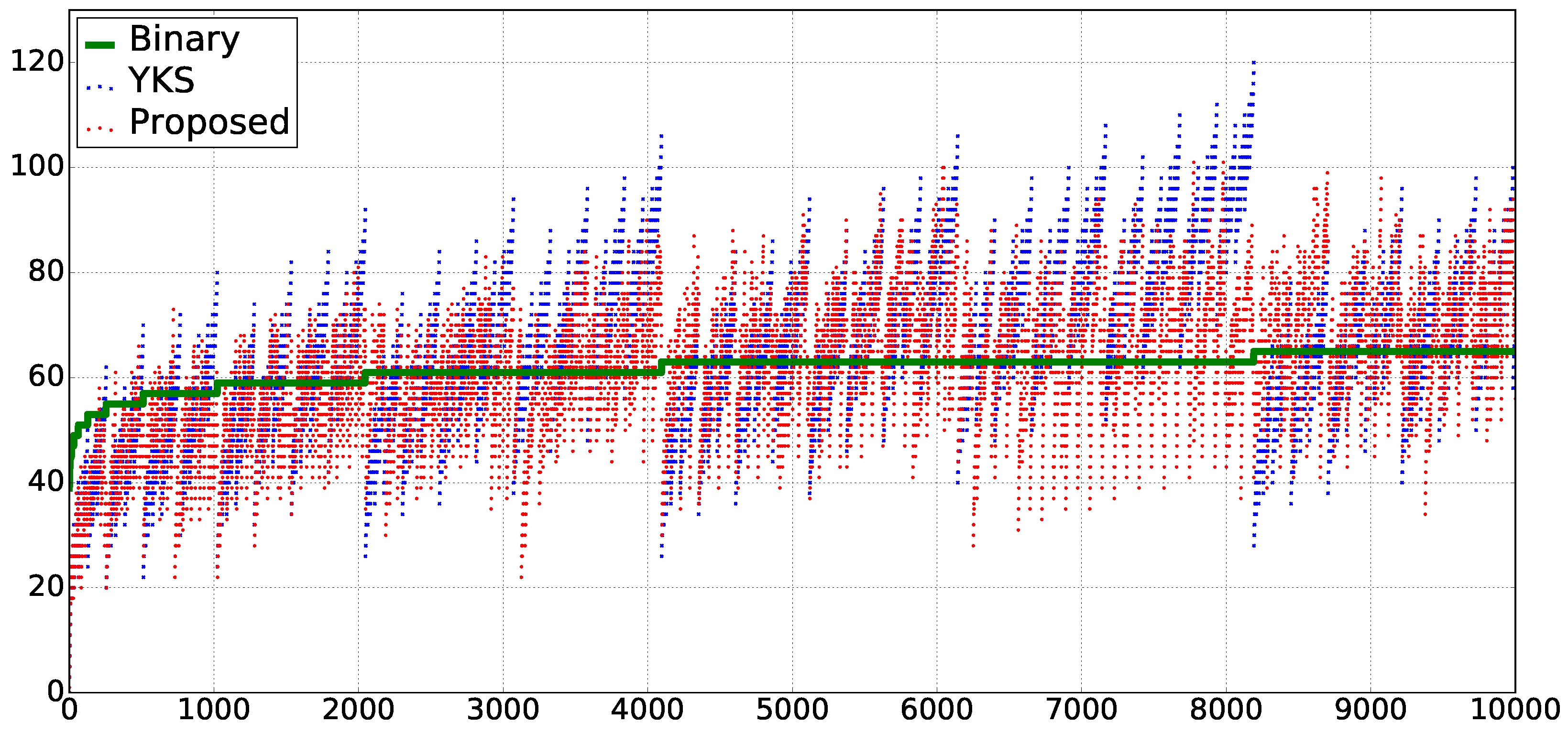
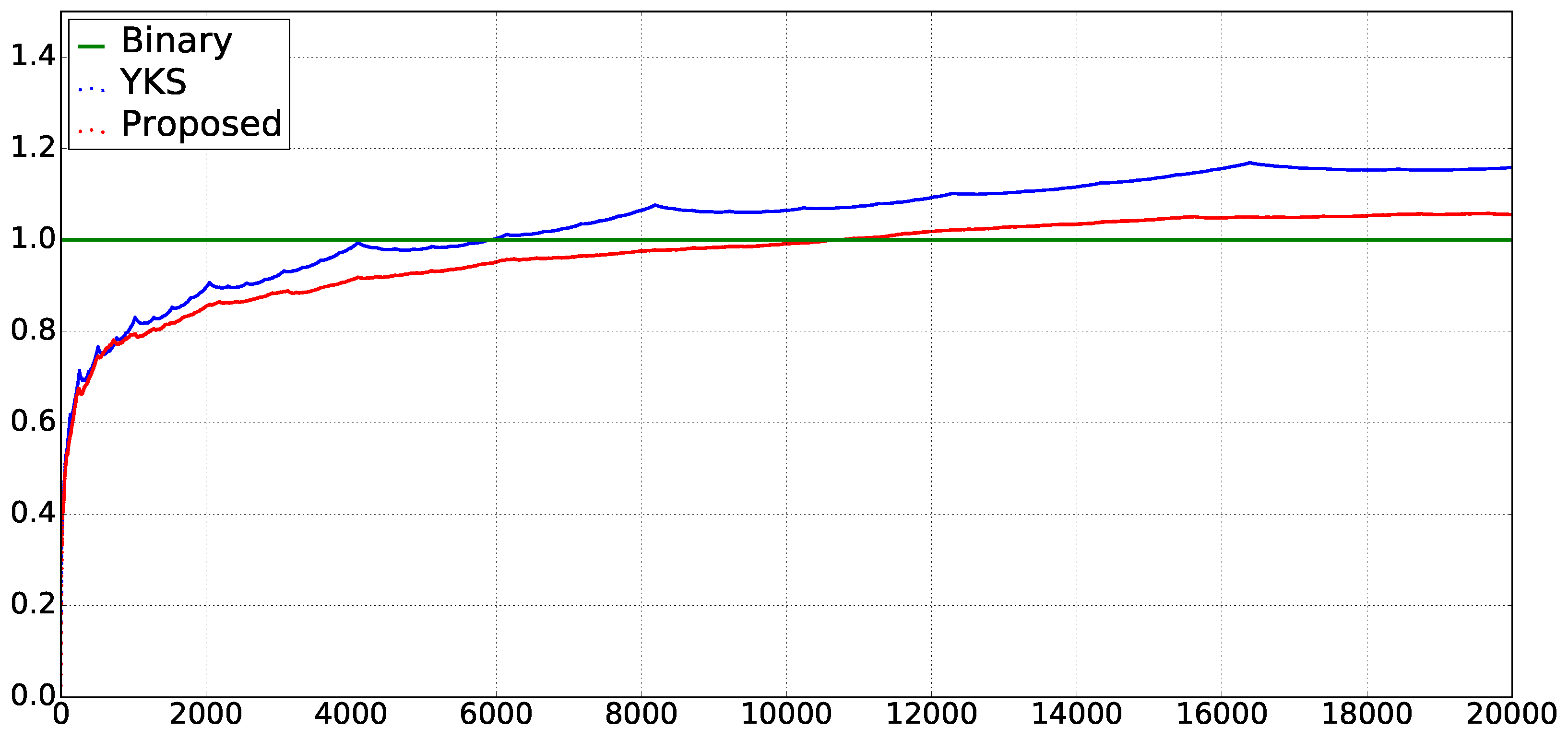
Figure 1 and Figure 2 show the experimental results. In both of them, “Binary”, “YKS”, and “Proposed” denote the methods using the binary expression on -terms, YKS, and ours, respectively. The horizontal axis shows the repetition number n of given text . Then, we compare the sizes of the generated extended -terms by using these three methods, for the given .
In Figure 1, the vertical axis shows the sizes of , , and . The inequality holds in 5187 out of 10,000 cases within the range . The average ratio for the range is approximately 0.9962. Similarly, the inequality holds in 5959 cases, and the average ratio is approximately 0.9321.
In Figure 2, the vertical axis shows the ratio (the average size of cumulative sum of extended -terms from 1 to n). That is, Figure 2 shows how and increase compared to on average. As can be seen, tends to be greater than when n is greater than 10,000. We consider that it is consistent with the theoretical upper bound , stated in Theorem 4.
5. Conclusions
In this paper, we addressed the problem of compaction of Church numerals. For given natural number n, by using proposed RTP, we decompose n into an arithmetic expression, which enables to obtain a compact -term leading to the Church numeral of n. We proved that the size of the obtained -term becomes . Moreover, we experimentally confirmed that the -terms produced by our method tend to be smaller than binary expressions on -terms on average, when the given number is less than approximately 10,000. We have not proved the lower bound of the size in the worst case; it is our future work.
The compaction of Church numerals can be applied to higher-order compression, that uses extended -terms as the data model. In the procedure of higher-order compression, a repetitive part in the input can be represented as a -term with . Thus, efficient compaction of will help for improving the compression performance of higher-order compression.
In data compression, data models are finally encoded in bit sequences. For bit encoding of -terms, Tromp [16] proposed a method for untyped -terms. Very recently, Takeda et al. [17] proposed an efficient encoding scheme for simply-typed -terms. Finding an efficient bit encoding for our method is also our future work.
Author Contributions
Conceptualization, I.F. and T.K.; Software, I.F.; Writing—original draft, I.F. and T.K.; Writing—review & editing, I.F. and T.K.
Funding
This work was supported by JSPS KAKENHI Grant Number JP15K00002, JP18K11149, JP18K19771 and JST CREST Grant Number JPMJCR1402, Japan.
Acknowledgments
The authors would like to thank Ayumi Shinohara and his colleagues for providing the source code for higher-order compression.
Conflicts of Interest
The authors declare no conflict of interest.
References
- Kobayashi, N.; Matsuda, K.; Shinohara, A.; Yaguchi, K. Functional programs as compressed data. High. Order Symb. Comput. 2012, 25, 39–84. [Google Scholar] [CrossRef]
- Yaguchi, K.; Kobayashi, N.; Shinohara, A. Efficient algorithm and coding for higher-rder compression. In Proceedings of the 2014 Data Compression Conference (DCC2014), Snowbird, UT, USA, 26–28 March 2014; p. 434. [Google Scholar]
- Kieffer, J.C.; Yang, E.H. Grammar-based codes: A new class of universal lossless source codes. IEEE Trans. Inf. Theory 2000, 46, 737–754. [Google Scholar] [CrossRef]
- Cover, T.M.; Thomas, J.A. Elements of Information Theory (Wiley Series in Telecommunications and Signal Processing); Wiley-Interscience: New York, NY, USA, 2006. [Google Scholar]
- Charikar, M.; Lehman, E.; Liu, D.; Panigrahy, R.; Prabhakaran, M.; Sahai, A.; Shelat, A. The smallest grammar problem. IEEE Trans. Inf. Theory 2005, 51, 2554–2576. [Google Scholar] [CrossRef]
- Larsson, N.J.; Moffat, A. Off-line dictionary-based compression. Proc. IEEE 2000, 88, 1722–1732. [Google Scholar] [CrossRef]
- Maruyama, S.; Tanaka, Y.; Sakamoto, H.; Takeda, M. Context-sensitive grammar transform: Compression and pattern matching. In Proceedings of the String Processing and Information Retrieval (SPIRE2008), Melbourne, Australia, 10–12 November 2008; pp. 27–38. [Google Scholar]
- Masaki, T.; Kida, T. Online grammar transformation based on re-pair algorithm. In Proceedings of the Data Compression Conference (DCC2016), Snowbird, UT, USA, 30 March–1 April 2016; pp. 349–358. [Google Scholar]
- Nevill-Manning, C.G.; Witten, I.H.; Maulsby, D.L. Compression by induction of hierarchical grammars. In Proceedings of the Data Compression Conference (DCC’94), Snowbird, UT, USA, 29–31 March 1994; pp. 244–253. [Google Scholar]
- Takabatake, Y.; Sakamoto, H. A space-optimal grammar compression. In Proceedings of the 25th Annual European Symposium on Algorithms (ESA 2017), Vienna, Austria, 4–6 September 2017; Leibniz International Proceedings in Informatics (LIPIcs). Volume 87, pp. 67:1–67:15. [Google Scholar] [CrossRef]
- Ohno, T.; Goto, K.; Takabatake, Y.; I, T.; Sakamoto, H. LZ-ABT: A practical algorithm for α-balanced grammar compressio. In Proceedings of the 29th International Workshop on Combinatorial Algorithms (IWOCA 2018), Singapore, 16–19 July 2018; Springer: Singapore, 2018; pp. 323–335. [Google Scholar]
- Rytter, W. Grammar compression, LZ-encodings, and string algorithms with implicit input. In Automata, Languages, and Programming (ICALP2004); Díaz, J., Karhumäki, J., Lepistö, A., Sannella, D., Eds.; Springer: Berlin/Heidelberg, Germany, 2004; pp. 15–27. [Google Scholar]
- Lohrey, M. Algorithmics on SLP-compressed strings: A survey. Groups Complex. Cryptol. 2012, 4, 241–299. [Google Scholar] [CrossRef]
- Furuya, I.; Kida, T. Compaction of church numerals for higher-order compression. In Proceedings of the Data Compression Conference (DCC2018), Snowbird, UT, USA, 27–30 March 2018; p. 408. [Google Scholar]
- Mogensen, T.A. An investigation of compact and efficient number representations in the pure lambda calculus. In Revised Papers from the 4th International Andrei Ershov Memorial Conference on Perspectives of System Informatics (PSI ’02): Akademgorodok, Novosibirsk, Russia; Springer-Verlag: London, UK, 2001; pp. 205–213. [Google Scholar]
- Tromp, J. Binary lambda calculus and combinatory logic. In Kolmogorov Complexity and Applications; Hutter, M., Merkle, W., Vitanyi, P.M., Eds.; Number 06051 in Dagstuhl Seminar Proceedings; Internationales Begegnungs- und Forschungszentrum fuer Informatik (IBFI): Schloss Dagstuhl, Germany, 2006. [Google Scholar]
- Takeda, K.; Kobayashi, N.; Yaguchi, K.; Shinohara, A. Compact bit encoding schemes for simply-typed lambda-terms. In Proceedings of the 21st ACM SIGPLAN International Conference on Functional Programming, Nara, Japan, 18–24 September 2016; Volume 51, pp. 146–157. [Google Scholar]
Figure 1.
Term size for integer n.

Figure 2.
Average ratio to binary expression.


Table 1.
n, , and for and .
| n | n | ||||
|---|---|---|---|---|---|
| 9 | 21 | 20 | 13 | 29 | 26 |
| 10 | 23 | 22 | 14 | 31 | 28 |
| 11 | 25 | 24 | 15 | 33 | 28 |
| 12 | 27 | 24 |
© 2019 by the authors. Licensee MDPI, Basel, Switzerland. This article is an open access article distributed under the terms and conditions of the Creative Commons Attribution (CC BY) license (http://creativecommons.org/licenses/by/4.0/).
Share and Cite
MDPI and ACS Style
Furuya, I.; Kida, T. Compaction of Church Numerals. Algorithms 2019, 12, 159. https://0-doi-org.brum.beds.ac.uk/10.3390/a12080159
AMA Style
Furuya I, Kida T. Compaction of Church Numerals. Algorithms. 2019; 12(8):159. https://0-doi-org.brum.beds.ac.uk/10.3390/a12080159
Chicago/Turabian StyleFuruya, Isamu, and Takuya Kida. 2019. "Compaction of Church Numerals" Algorithms 12, no. 8: 159. https://0-doi-org.brum.beds.ac.uk/10.3390/a12080159
Note that from the first issue of 2016, this journal uses article numbers instead of page numbers. See further details here.