Algorithmic Matching Attacks on Optimally Suppressed Tabular Data

1
Department of Statistical Science, School of Multidisciplinary Sciences, The Graduate University for Advanced Studies (SOKENDAI), Shonan Village, Hayama, Kanagawa 240-0193, Japan
2
The Institute of Statistical Mathematics, 10-3 Midori-cho, Tachikawa, Tokyo 190-8562, Japan
3
National Statistics Center, 19-1 Wakamatsu-cho, Shinjuku-Ku, Tokyo 162-8668, Japan
*
Author to whom correspondence should be addressed.
Algorithms 2019, 12(8), 165; https://0-doi-org.brum.beds.ac.uk/10.3390/a12080165
Submission received: 30 June 2019
/
Revised: 6 August 2019
/
Accepted: 8 August 2019
/
Published: 11 August 2019
(This article belongs to the Special Issue Statistical Disclosure Control for Microdata)
Abstract
:The objective of the cell suppression problem (CSP) is to protect sensitive cell values in tabular data under the presence of linear relations concerning marginal sums. Previous algorithms for solving CSPs ensure that every sensitive cell has enough uncertainty on its values based on the interval width of all possible values. However, we find that every deterministic CSP algorithm is vulnerable to an adversary who possesses the knowledge of that algorithm. We devise a matching attack scheme that narrows down the ranges of sensitive cell values by matching the suppression pattern of an original table with that of each candidate table. Our experiments show that actual ranges of sensitive cell values are significantly narrower than those assumed by the previous CSP algorithms.
1. Introduction
The cell suppression problem (CSP) [1] has been studied for many years to properly protect sensitive information in tabular data. The goal of CSP is to determine a set of suppressed cells that ensure sufficient uncertainty of the values of sensitive cells under the presence of linear relations concerning marginal sums in the table. Since CSP is known to be NP-hard, many researchers have previously developed efficient approximate or heuristics-based algorithms [2,3,4]. Particularly, the algorithm [1] based on the technique of Benders decomposition [5] has been adopted for tools for statistical disclosure control (SDC), such as -ARGUS [6], SDCLink [7] and sdcTable [8], because that algorithm guarantees to produce optimal solutions while running efficiently in many realistic situations.
Previous research on CSP [9] has defined the safety of a suppressed table based on the notion of a feasibility interval. We represent a suppressed cell by a variable that takes an unknown value and examine the set of all possible values for that variable. When multiple variables are subject to linear constraints in CSP, the range of each variable becomes a linear segment between two end points. We call such a segment the feasibility interval of a cell variable and quantify the safety of the corresponding suppressed cell based on the width of the interval. Previous research [1] considers a suppressed cell safe if the width of its feasibility interval is greater than a given threshold. To obtain the feasibility interval of a suppressed cell, we solve two linear programming problems to obtain the minimum and the maximum bounds of that cell variable subject to the linear constraints of marginal sums. The previous algorithms implicitly consider each combination of values for suppressed cells feasible as long as those values satisfy the constraints of marginal sums.
However, we find that it is possible to exclude some feasible combinations of values of suppressed cell variables if we know that a deterministic CSP algorithm (e.g., References [2,10]) is used to suppress the original table. We can construct a candidate table of the original table by complementing its suppressed cells with a feasible combination of cell values. If we apply the same suppression algorithm to the candidate table, we are supposed to reproduce the same suppressed table. Otherwise, we conclude that that particular combination of cell values never coincide with the suppressed cell values of the original table. Since it is possible to enumerate all feasible combinations of suppressed cell values by solving indefinite linear equations of marginal constraints involving cell variables, we devise a systematic way of narrowing down the ranges of the feasibility intervals. In this paper, we assume an adversary who tries to infer sensitive cell values in a publicly released suppressed table and that the adversary possesses the knowledge of the CSP algorithm observing the Kerckhoffs’ principle [11].
We develop a matching attack for computing the effective feasibility intervals of suppressed cells in tabular data. The main idea is to compute the feasibility intervals of suppressed cells incrementally while performing the matching test on the suppression pattern of each candidate table. If a candidate table reproduces the suppression pattern of the original table, we consider that the cell values of that candidate table feasible and expand the ranges of their effective feasibility intervals accordingly. We assume that a deterministic CSP algorithm applies a pre-determined threshold for the minimum width of a feasibility interval to each sensitive cell of a table. We find that the number of feasible combinations of cell values largely depends on the dimension of the null space of a matrix representing the linear constraints of the original table. That is, when the dimension of the null space is small, the width of an effective feasibility interval is often significantly narrower than that assumed by the CSP algorithm violating the security requirement of the minimum interval width.
We evaluate the effectiveness and computational performance of the proposed matching attack with a large number of synthetically generated frequency tables in which the sensitivity of each cell is determined by comparing its value with a given minimum frequency threshold. We use our implementation of the CSP algorithm [7], which ensures a given minimum width threshold on the feasibility interval of each sensitive cell. Our experiments demonstrate that the matching attacks are both feasible and practical for tables of small and medium sizes compromising the safety of about 46% to 83% of the sensitive cell values.
We summarize our contributions in this paper as follows:
- We devise the new matching attack scheme on a suppressed table to narrow down the ranges of sensitive cell values exploiting the fact that some algorithms for CSP are deterministic.
- We implement the matching attack, which systematically enumerates all the combinations of candidate values for suppressed cells, performs the matching test on each candidate table and computes the effective feasibility intervals of sensitive cells.
- We experimentally show that the proposed attack is effective to a large number of synthetically generated frequency tables and that there is a significant risk of many sensitive cell values being identified exactly.
The rest of the paper is organized as follows. Section 2 describes the formulation of the CSP introducing the notion of the feasibility interval, based on which we determine the safety of suppressed tabular data. We finally define our adversary model justifying our assumptions on the capability of an adversary. Section 3 describes the matching attack that systematically examines all candidate tables and performs the matching test, and Section 4 demonstrates the effectiveness of the matching attacks experimentally. Section 5 discusses related work and Section 6 concludes.
2. Background
In this section, we first formulate the cell suppression problem (CSP) introducing the notion of the feasibility interval. Previous algorithms for CSP implicitly use the safety definition for suppressed tables based on the minimum width of the feasibility intervals of sensitive cells. We next define the adversary model, justifying our assumptions on an adversary’s knowledge on the CSP algorithm and its security parameters for inputs to the algorithm.
2.1. Disclosure Risks in Tabular Data
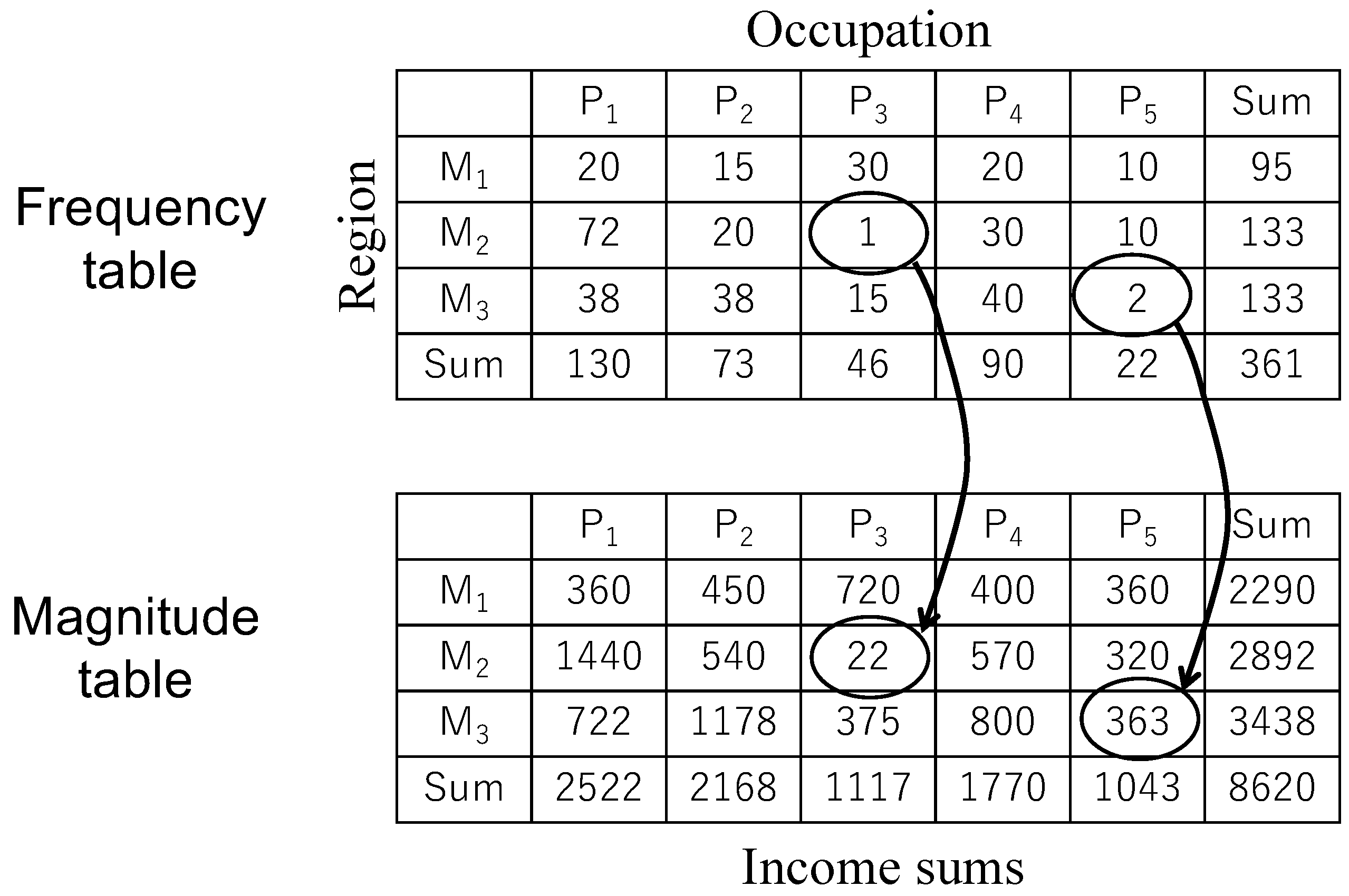
We first describe disclosure risks in tabular data, which contain sensitive information on individuals. Tabular data are produced from microdata that consist of records of an individual respondent’s variables (i.e., attributes) such as age, income and so on. There are two types of tabular data—frequency tables and magnitude tables. Both types of tables classify records of microdata into a set of cells that correspond to a particular value combination of grouping variables. For example, Figure 1 shows a pair of frequency and magnitude tables whose cells are crossed by two variables M and P. The variables M and P represent a geographical region where the respondent of a record resides and that respondent’s occupation, respectively. Both variables are categorical variables whose domains are a finite set of discrete values. The frequency table on the left shows the numbers of respondents that belong to each cell of the table. The magnitude table on the right shows the income sums of those in each cell. We here assume that there is another quantitative variable income I in each record of the microdata.
Now we suppose that an adversary knows that someone possesses attributes and and that that person’s record is included in the tables in Figure 1. Those attributes of a person are easily observable to her neighbors. Since there is a single respondent with the attributes and , the adversary can identify that respondent uniquely. If the adversary also obtains the magnitude table in Figure 1, he can infer the exact amount of salary of the identified respondent, which appears in cell of the magnitude table. Therefore, a respondent who belongs to a cell of a single unit has a significant risk of disclosing his sensitive information to an adversary who can learn some of the respondent’s attributes. Similarly, there is a disclosure risk in a cell with a small number of units. For example, consider cell with two units in the frequency table in Figure 1. This time, we assume an internal adversary who himself contributes to cell as a respondent. If he can identify another respondent in cell by knowing his attribute values, the adversary can infer the income of that respondent by subtracting the amount of his salary from the value in of the magnitude table. In general, we model an adversary as a set of colluding respondents who contribute their records to tabular data and thus consider cells with low frequency in a table unsafe.
2.2. Overview of the Cell Suppression Problem (CSP)
We protect sensitive information in tabular data by suppressing the values of unsafe cells that are determined by applying some sensitivity rule [9] to each cell of the table. For example, we apply the minimum frequency rule to a frequency table such that each cell will be suppressed if its value is less than a given threshold for the minimum frequency. We call this process primary suppression and call suppressed cells in primary suppression primary suppressed cells accordingly. However, to perform primary suppression on a table is not sufficient to protect sensitive cell values because it is usually trivial to restore the original values by utilizing linear relationships among cell values concerning marginal sums. We, therefore, perform secondary suppression that additionally suppresses the values of non-sensitive cells to prevent an adversary from recomputing the cell values of primary suppressed cells. We call non-sensitive cells that are suppressed in secondary suppression secondary suppressed cells.
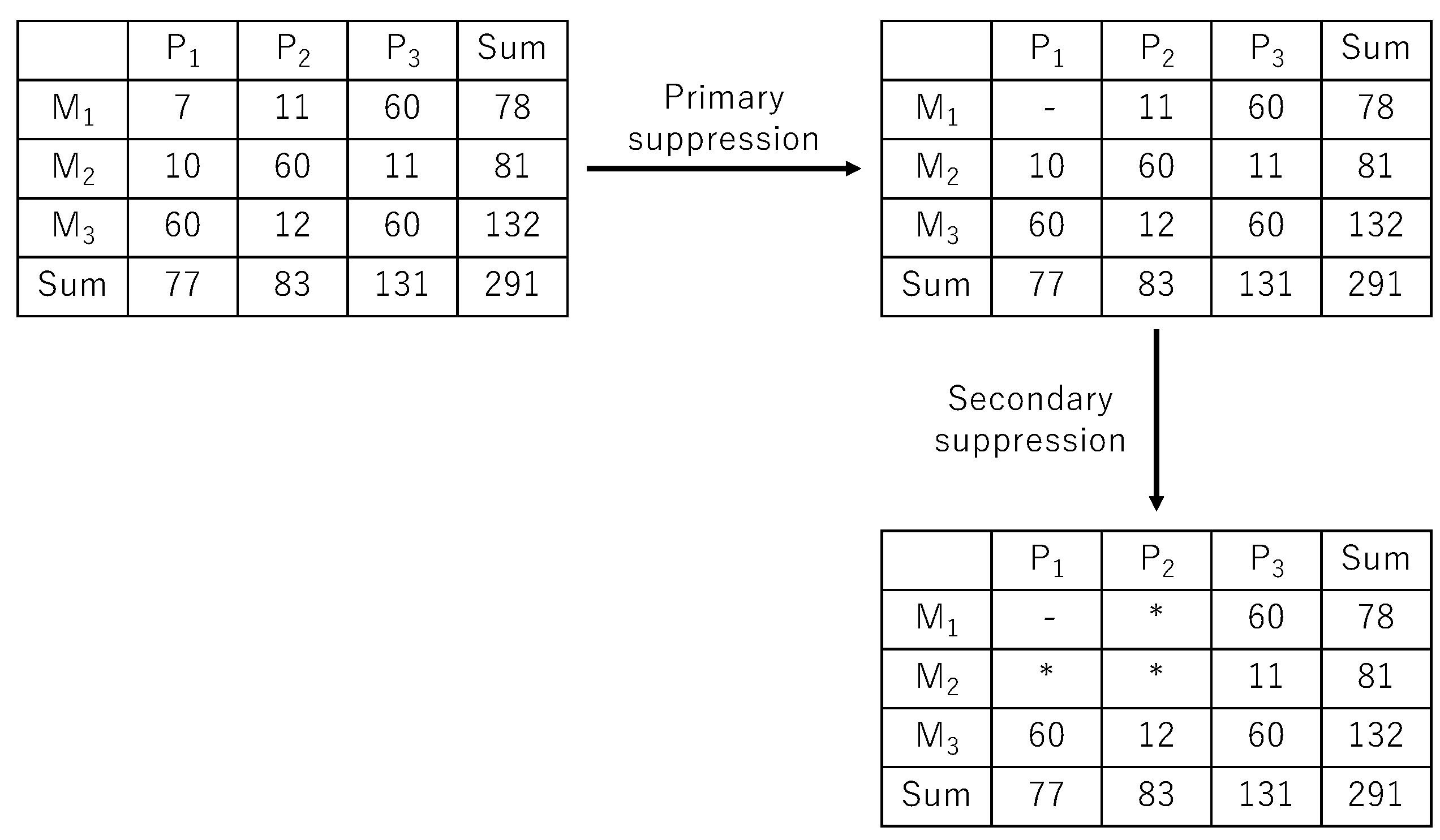
We illustrate this two-stage cell suppression procedure with an example of a frequency table in Figure 2. We first determine sensitive cells using the minimum frequency rule with a threshold value of 10. In this example, we determine that cell (, ,) is sensitive and suppress that cell value in the process of primary suppression. Since it is trivial to restore the suppressed value by considering a linear relationship either on the row sum or the column sum, we additionally suppress three non-sensitive cells (, ), (, ), and (, ).
It is, however, not clear whether this particular choice of secondary suppressed cells adequately protects sensitive information in the primary suppressed cell. Also, we need to minimize information loss due to secondary suppression while protecting the value of the primary suppressed cell. We therefore define CSP at a high level as follows:
Definition 1 (Cell Suppression Problem (CSP)).
Given a secondary suppressed table T and a set S of primary suppressed cells in T, CSP determines a setof secondary suppressed cells with the minimum information loss under the constraint that the value of each primary suppressed cellis properly protected.
We next describe the security definition on a primary suppressed cell in Section 2.3 and formulate the optimization problem of minimizing information loss in the framework of integer linear programming (ILP) in Section 2.2.
2.3. Safety of Suppressed Tabular Data
To determine whether a given choice of secondary suppressed cells properly protects the values of primary suppressed cells, we need to verify that each primary suppressed cell has enough uncertainty on its value under the presence of linear relations concerning marginal sums. We consider a two-dimensional table T of r rows by c columns without loss of generality. Figure 3 shows linear relations in table T. We denote by the value of cell in T and express the linear relations on marginal sums as follows:
We also assume that every cell takes a non-negative value as in the case of a frequency table, that is,
Suppose that we suppress some cells in T and obtain a suppressed table . To quantify the uncertainty of suppressed cell values in , we introduce a cell variable for each cell of . We also introduce the notion of a suppression pattern y, which is a binary matrix of the same size as table . The suppression pattern y specifies which cells in table are suppressed such that:
We can obtain the lower bound of each primary suppressed cell by solving the ILP problem below.
Equation (8) sets the value for to be the actual cell value if that cell is suppressed in , which is indicated by the value in suppression pattern y. Similarly, we can obtain the upper bound of cell by computing the maximum value of under the same constraints (6)–(9) of the above ILP problem.
We now define the feasibility interval of a suppressed cell in table as follows.
Definition 2 (Feasibility interval).
Given a suppressed tablewith a suppression pattern y, the feasibility interval for a suppressed cellis an intervalbetween the lower and upper bounds of cell variableand its width is defined as the delta between the two end points; that is,
We quantify the uncertainty of a primary suppressed cell with the width of its feasibility interval and require that the width of the feasibility interval of every primary suppressed cell is greater than a given threshold value for the minimum width, as shown in Figure 4.
We consider that a suppressed table is safe if every primary suppressed cell in is safe.
Definition 3 (Safety of a suppressed table T′).
Given a suppressed tablewith a suppression pattern y, a set of primary suppressed cells P, and a minimum threshold δ, we say that a tableis safe if, for every primary suppressed cell,
holds.
Example 1.
Consider the secondary suppressed tablein Figure 2. Suppose that the minimum width δ for feasibility intervals is 10. we compute the lower and upper boundsandof the primary suppressed cellwith the following constraints.
which can be simplified by eliminating variables for non-suppressed cells as follows.
By solving the two problems of ILP, we obtain and respectively. Therefore, the feasibility interval . Since a cell is the only primary suppressed cell in , we conclude that table is safe.
2.4. Cell Suppression Problem (CSP)
We now formulate the CSP. Obviously, the more we suppress cells in a table, the greater the uncertainty of the value of each suppressed cell is and thus the safer the table is. However, if we suppress too many cells, the suppressed table with such significant information loss is not useful for any data analysis. Therefore, we aim to minimize information loss due to secondary suppression. The goal of solving a CSP for a given table is to determine the minimum set of cells to be suppressed that is sufficient to protect sensitive information in primary suppressed cells.
We formulate CSP as an optimization problem of minimizing information loss under the safety condition in Definition 3 as follows.
Definition 4 (Cell suppression problem (CSP)).
Given a table T, a set of primary suppressed cells P, and a threshold δ for the minimum width of a feasibility interval, a CSP determines the suppression pattern y such that:
whereis the width of cell’s feasibility interval in Definition 2.
2.5. Adversary Model
An adversary in this paper tries to infer sensitive cell values in a publicly released table. We assume that such an adversary knows the suppression algorithm for solving CSPs based on the Kerckhoffs’ principle [11], which is one of the basic principles in cryptography. -ARGUS [6], which is a software program for solving a CSP, are publicly available with its source code and manual [12] that describes the algorithms in detail. We also assume that an adversary knows security parameters, such as threshold values for the minimum frequency of cell values and the minimum width of a feasibility interval, because researchers who conduct data analysis on microdata at a secure on-site (e.g., [13]) need to know output checking rules to get a permission from an output checker at a statistics office to bring their produced tables back home. For example, Statistics Netherlands publishes reference guidelines for output checking [14], which mentions 10 units as the minimum frequency of cell values in frequency tables. National Statistics Center in Japan publishes information on output checking rules including security parameters for tabular data at [15].
Even if a statistics agency keeps security parameters secret, an adversary can narrow down the ranges of those parameters by examining published suppressed tables, which are determined to be safe. We argue that security by obscurity does not work for CSP because the ranges of those security parameters are significantly smaller than key space in cryptography and we cannot change security parameters randomly as we do for a secret key in cryptography when they are disclosed by malicious insiders. The adversary can utilize the fact that a threshold for the minimum frequency must be smaller than any cell value of a published table and that a threshold for the minimum width of a feasibility interval must be smaller than the feasibility interval of any suppressed cell in published tables. Remember that the feasibility interval of each suppressed cell can be computed by solving the two linear programming problems in Equations (5)–(9).
3. Matching Attack
In this section, we describe the matching attack that eliminates a subset of candidate tables whose suppression patterns generated by the same CSP algorithm do not match with that of the original table. The attack computes the effective feasibility interval of each suppressed cell in the original table by only considering the range of cell values in the matched candidate tables. The width of an effective feasibility interval is possibly smaller than that defined in Definition 2, violating the safety property in Definition 3. Note that our attack is applicable only to frequency tables in which a threshold for the minimum width of the feasibility interval of each sensitive cell is determined independently of cell values in a table.
3.1. Overview of the Matching Attack
We describe the matching attack on a secondary suppressed table produced by a deterministic CSP algorithm. Our attack exploits the fact that such a deterministic algorithm always outputs the same suppressed table from the same input table. For example, the optimal algorithm [10] and the network flow algorithm [2] in -ARGUS and the algorithm in SDCLink [7] are deterministic. The R package sdcTable [8] uses one of the CSP algorithms in -ARGUS underneath to solve a CSP.
Figure 5 shows a conceptual scheme of the matching attack. An adversary first obtains the original suppressed table and enumerates every possible candidate table of the original table by complementing the suppressed cells of the suppressed original table with values that satisfy the constraints in (1), (2), and (3). The adversary next applies the CSP algorithm to each candidate table. We here assume that the adversary knows the CSP algorithm and its security parameters as described in Section 2.5. If a resulting suppressed table is the same as the suppressed original table, we consider that candidate table a real candidate; otherwise, we eliminate it from the list of candidate tables.
The main idea of the attack is to recompute the feasibility intervals of the suppressed cells in the suppressed original table by only considering the range of cell values in the matched candidate tables. We call the feasibility intervals recomputed with the real candidate tables the effective feasibility intervals. On the other hand, the feasibility interval in Definition 2 considers all candidate tables satisfying the linear and non-negativity constraints. Therefore, the width of the effective feasibility interval of a suppressed cell could be smaller than that of the feasibility interval in Definition 2 such that an adversary can infer that cell value more accurately than assumed by the CSP algorithm.
3.2. Enumerating Candidate Tables
We enumerate candidate tables by obtaining solutions of indefinite equations (1) and (2) involving cell variables of suppressed cells in the original table. We assume that cell variables for non-suppressed cells are replaced with the actual cell values as we do in Example 1 in Section 2.3. We denote the linear equations in (1) and (2) in a matrix form as follows.
where A is the coefficient matrix, x is a column vector of cell variables, and b is a column vector of marginal sums either on a row or a column. We here assume that we order cell variables in a table in a sequential order either by row or column.
Let be the null space of matrix A such that
where n is the number of cell variables and is the set of integers. If are solutions to , that is and , then . Thus, the difference between any two solutions belongs to the null space . Therefore, any solution to the equation can be expressed as the sum of a fixed solution v and some element in ; that is, the set S of all solutions to is defined as follows.
Since the null space is represented by the linear combinations of independent vectors, we can enumerate all possible solutions that satisfy the non-negative constraints in (3) systematically.
Example 2.
Suppose that we have a suppressed table in Table 1. There are four suppressed cells whose cell variables are, , , and , respectively.
Since each variable takes a non-negative value, we represent the set S of all possible combinations of cell values as
In this example, the dimension of the null space is 1, but, in general, the null space is represented as a linear combination of multiple column vectors.
3.3. Algorithm for the Matching Attack
Our attack computes the effective feasibility interval of each suppressed cell by considering the cell values of candidate tables whose suppression pattern matches with that of the original table. We formally define the effective feasibility interval of a suppressed cell as follows.
Definition 5 (Effective feasibility interval).
Suppose that the functionfor solving a CSP takes a tableand a list of security parametersas inputs and outputs a suppressed table. Given a suppressed table, the functionand its security parameters, the effective feasibility interval for a suppressed cellis defined aswhere
The widthof the effective feasibility intervalis defined as
Algorithm 1 shows the pseudocode of the matching attack, which computes the effective feasibility intervals of suppressed cells in Definition 5. The algorithm takes a suppressed table , a minimum frequency t and a threshold width for the minimum width of the feasibility interval of a suppressed cell as inputs and outputs a list of actual feasibility intervals for the suppressed cells in the input table .
Line 1 obtains a list of cell variables in a suppressed table . Each variable has an entry , which maintains its minimum and maximum values. Lines 2–5 initialize each variable ’s minimum and maximum values to ∞ and 0, respectively. Line 6 generates the linear equations of a matrix form (32) from the input suppressed table by calling the function , which produces the coefficient matrix A representing the linear equations regarding marginal row sums and column sums. Lines 7 obtains a fixed solution v to linear equations by calling the function , which chooses the solution v closest to the origin of the coordinate system. We implement this function using the package [16] for ILP in the R language. Line 8 computes the null space with the function . We represent the null space of A by the span of column vectors in . Line 9 enumerates all candidate solutions to where for all i and put them into set S. The function adds each linear combinations of column vectors in into the fixed solution v and put into set S if all the components of the resulting solution take a non-negative value as specified in (34).
| Algorithm 1 Function |
| Input: a suppressed table: , a minimum frequency t, a threshold width: Output: a set of actual feasibility intervals for the suppressed cells:
|
The for loop in lines 10–22 performs the matching test on every candidate table and incrementally obtain the effective feasibility interval of each suppressed cell in . Line 11 prepares a candidate table by complementing suppressed cells in with each solution s in the set S of all solutions. Line 12 performs cell suppression on a candidate table with the function for solving a CSP. As we discuss the adversary model in Section 2.5, we assume that an adversary uses the same deterministic algorithm and security parameters t and as is used to produce an input suppressed table . Line 13 checks whether a suppressed candidate table is same as the input table . If so, lines 14–20 updates the feasibility intervals of each suppressed cell if the candidate cell values are outside the current ranges of the feasibility intervals. After examining all possible solutions for cell variables, line 23 returns a list of variables with their effective feasibility intervals.
4. Evaluation of the Matching Attacks
We evaluate the effectiveness of the matching attack in Section 3.1 experimentally using synthetically generated tables. We measure how the matching attack narrows down the widths of the feasibility intervals of primary suppressed cells by comparing them with those of the effective feasibility intervals computed by Algorithm 1.
4.1. Setup
We implement the matching attack in Algorithm 1 in the R language. The program consists of about 700 lines of code in total. Also, to implement the function in that algorithm, we use our implementation of the program for solving CSP based on the technique of Benders decomposition [5] in the R language [7]. We prepare synthetic two-dimensional frequency tables for the experiments as follows. We prepare 50 square tables of the same size in terms of the number of cells. We vary the number of cells, 16, 25, 36, and 49. We set the value of each cell in those tables to a randomly drawn from a Gaussian distribution with the average 15 and the standard deviation 10. We choose a threshold for the minimum frequency to be 5 and choose a threshold for the minimum width of the feasibility interval of every sensitive cell to be 8.
We perform cell suppression on each synthetic table using the CSP algorithm and produce the secondary suppressed table . We next perform the matching attack in Algorithm 1 on with the same security parameters. We conduct our experiments on a Mac pro with the 3.5 GHz 6-Core Intel Xeon E55 processor and 64 GB main memory.
4.2. Safety of Primary Suppressed Cells
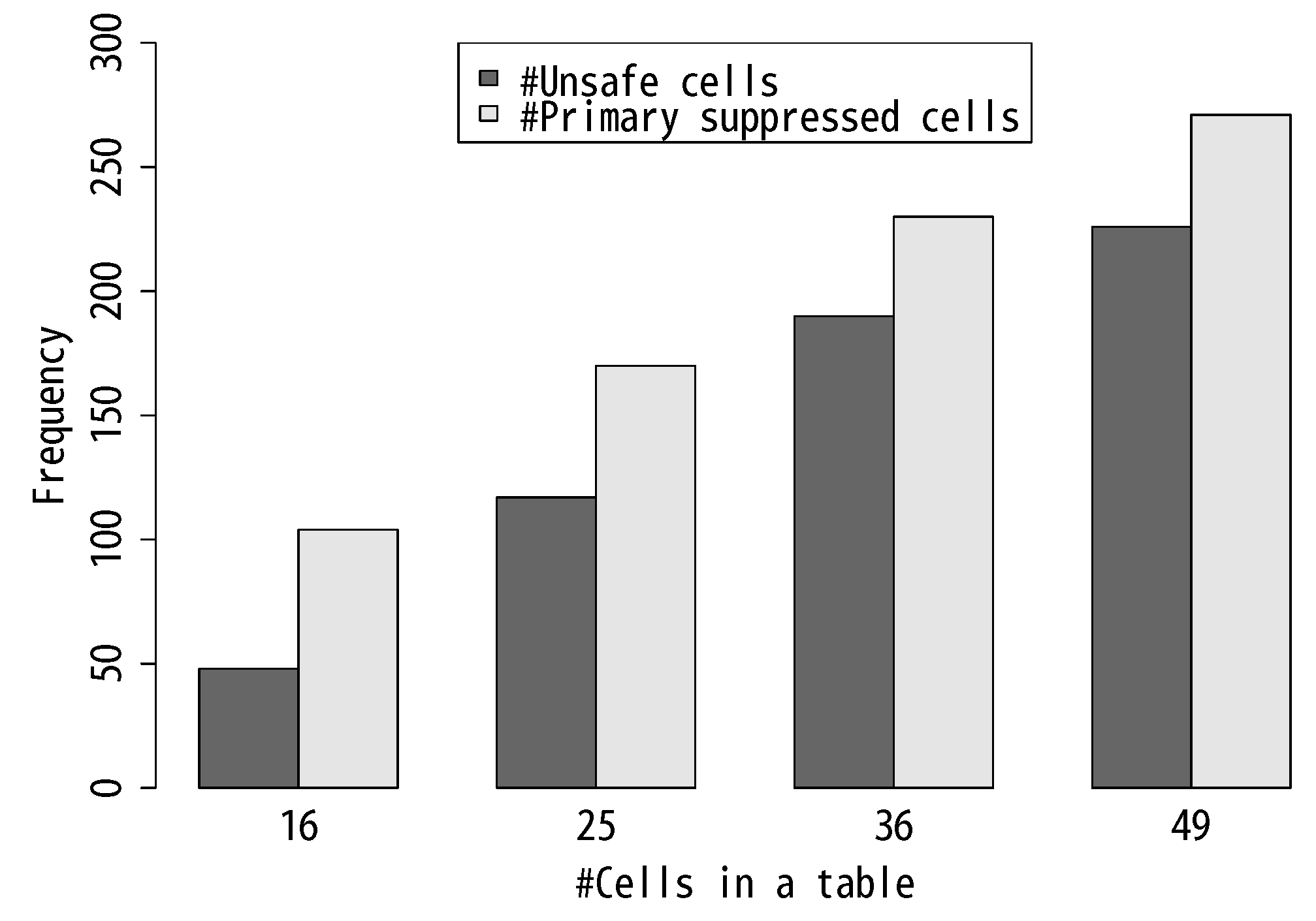
We first evaluate how many primary suppressed cells in the test tables are unsafe; that is, the widths of their effective feasibility intervals are smaller than the minimum width of 8 in the case of our experiments. Table 2 shows the ratios of unsafe primary suppressed cells whose effective feasibility intervals become shorter than the threshold for the minimum width. The ratio for each table size is computed by dividing the sum of unsafe primary suppressed cells by the sum of all primary suppressed cells in 50 test tables of that size. The bar chart in Figure 6 displays the same results graphically. The results show that about 46% to 83% of primary suppressed cells violate the safety requirement in Definition 3. We observe that, as the size of a table becomes larger, the ratio of unsafe cells increases.
We next examine how the ratio of unsafe cells depends on the dimension of the null space of the coefficient matrix A of a suppressed table in Section 3.2. Table 3 shows the ratios of unsafe cells by crossing tables with the dimensions of the null spaces and the number of cells in those tables. The results show that the lower the dimension of the null space is, the higher the risk of having unsafe cells in the table.
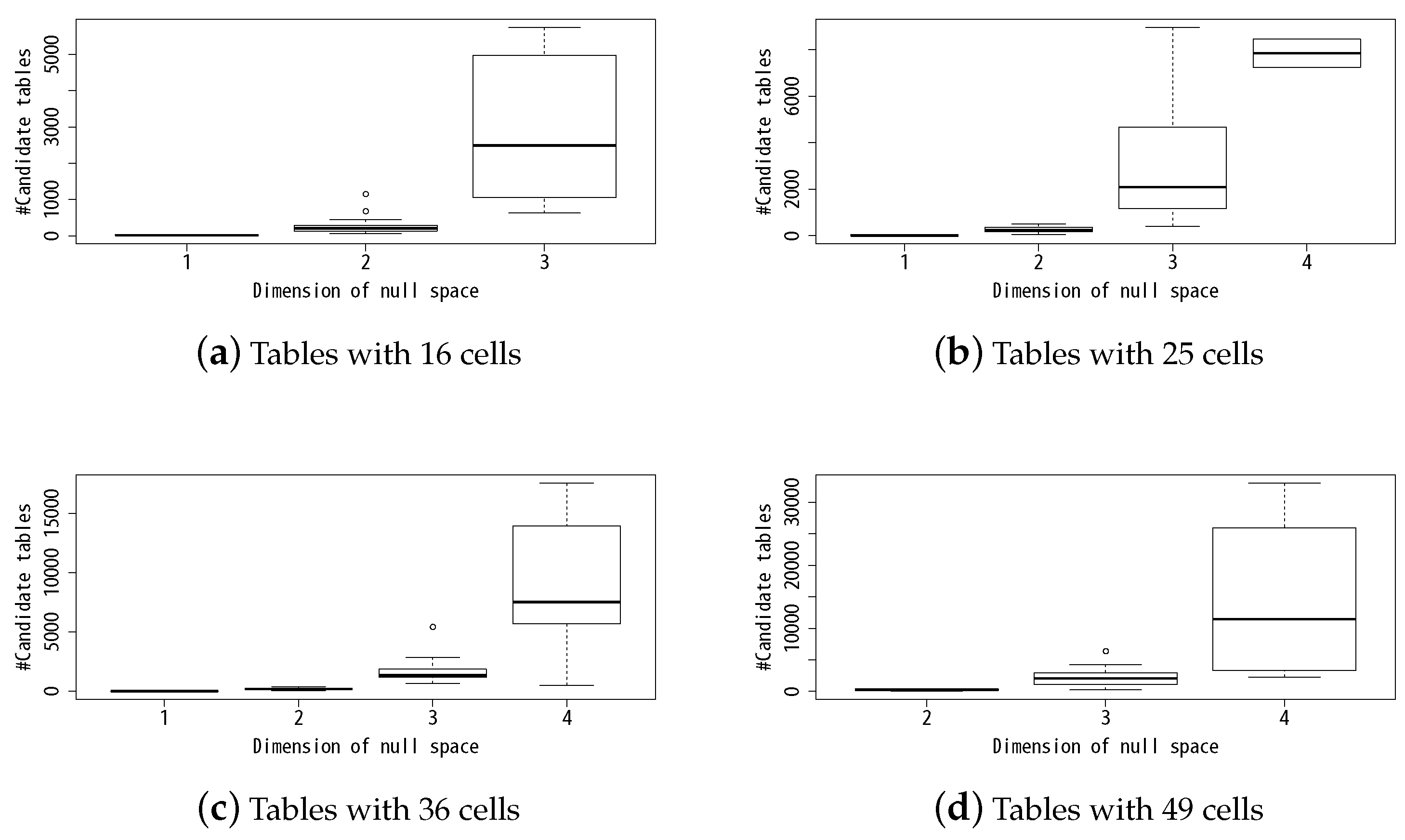
Figure 7 shows the number of candidate tables in dependence to the dimension of the null space of a suppressed table in box plot graph. We show the results for each size of tables. We see that when the dimension of the null space of a suppressed table is low, there are only a small number of possible combinations of cell values, and, therefore, the widths of the effective feasibility intervals of the suppressed cells become very slim.
4.3. Distributions of the Widths of the Effective Feasibility Intervals of Unsafe Cells
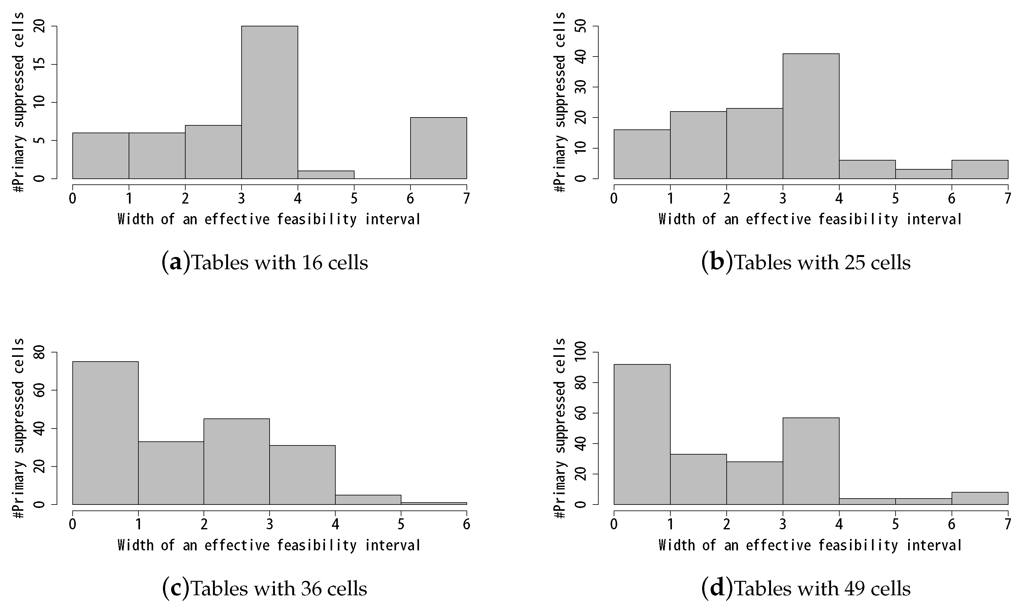
We next examine how accurately we can infer the ranges of unsafe cells. Table 4 shows the distributions of the widths of the effective feasibility intervals of unsafe primary suppressed cells. We show the same results in histograms in Figure 8. Surprisingly, we are able to determine the exact values of about 40% of the unsafe cells in tables of 36 cells and 49 cells. These results show that there are significant risks of revealing the exact values of sensitive cells under the presence of the matching attack.
4.4. Efficiency of the Attacks
We evaluate how efficiency we can perform matching attacks. We measure the average latency of executing the matching attacks in Algorithm 1 on 50 different suppressed synthetic tables for each table size. We use the function in the R language. Table 5 shows the average latency for tables of varying number of cells from 16 to 36. We see that the average latency increases exponentially as the table size grows because the numbers of the combinations of candidate cell values grow exponentially and the CSP algorithm based on the Benders decomposition is an exponential-time algorithm in the worst case. However, we believe that the matching attack is feasible with many of the publicly published tables that contain only small number of suppressed cells.
5. Related Work
To the best of our knowledge, there is no previous work on algorithmic attacks on optimally suppressed tabular data.
However, several researchers [17,18] study the issue of algorithm-based attacks on anonymized microdata in the context of privacy-preserving data publishing. The standard safety metrics for anonymized microdata is k-anonymity [19] and its variants (e.g., [20,21]). The k-anonymity model classifies tuple attributes into three categories: identifiers, quasi-identifiers (QIDs), and sensitive attributes, and defines the notion of equivalence class where all tuples in the same class possess the same set of values for the QIDs. The metrics of k-anonymity is syntactic in the sense that it requires that the size of every equivalence class is greater than a given threshold k. Many k-anonymity algorithms [22,23,24,25,26] are designed to achieve this property by generalizing values in QIDs while minimizing information loss.
Wong et al [17] observes that most anonymization algorithms adopt the minimality principle to minimize information loss based on some criteria, and shows that sensitive information could be revealed from anonymized data based on the privacy metrics of l-diversity [20] if an adversary knows that the algorithm divides tuples into equivalence classes depending on the values of sensitive attributes. They also propose the primary metrics m-confidentiality that guarantees that an adversary who additionally possesses the knowledge on the anonymization algorithm cannot have confidence of more than 1/m on an individual’s sensitive attribute value.
Although the concept of m-confidentiality is similar to safety conditions on feasibility intervals, which are extended to support continuous or ordered values, there is no efficient and systematic way of solving the inverse problem to verify the conditions of m-confidentiality. It is in general necessary to execute the anonymization algorithm with all possible instances of input microdata. On the other hand, our contribution in this paper is to show experimentally that it is possible to eliminate a large portion of possible candidate tables that could be an input to the CSP algorithm by conducting the matching test.
Jin et al. [18], who are also motivated by the issue of information disclosure from l-diversified anonymized data, establishes the requirements for algorithm-safe anonymization. The algorithm-safe anonymization guarantees that the conditional probability on a given instance of original microdata does not change even if the knowledge on the anonymization algorithm is added to the conditional premise. Although they also identify conditions for algorithm-safe anonymization, that result is not directly applicable to algorithms for CSP. It is still not clear how to generate safe suppressed frequency tables under the presence of the matching attack.
6. Conclusions
In this paper, we describe the novel matching attack to infer sensitive cell values of a suppressed table exploiting the fact that the CSP algorithm, which is used to suppress a target table, is deterministic. The key idea is to eliminate candidate tables whose suppression patterns do not match with that of the target table. We experimentally demonstrate that the matching attack is successful to narrow down the ranges of a large portion of sensitive cell values to be smaller than the specified minimum width of their feasibility intervals. We show that when the dimension of the null space of the coefficient matrix of a target table is low, there is significant risks of having unsafe cells whose values can be inferred accurately within a small range. As future work we plan to explore the possibility of developing a non-deterministic algorithm for CSP, which is resilient to the matching attack in this paper.
Author Contributions
K.M. devised the propsed attack scheme and implemented that attack method in the R languages. Y.A. conducted experiments and data analysis for evaluation.
Funding
This work was supported by KAKENHI (Grant-in-Aid for Scientific Research A) Grant Number 16H02013 from Japan Society for the Promotion of Science (JSPS) and “Challenging Exploratory Research Projects for the Future” grant from Research Organization of Information and Systems (ROIS).
Conflicts of Interest
The authors declare no conflict of interest.
Abbreviations
The following abbreviations are used in this manuscript:
| CSP | Cell suppression problem |
| ILP | Integer linear programming |
References
- Castro, J. Recent advances in optimization techniques for statistical tabular data protection. Eur. J. Oper. Res. 2012, 216, 257–269. [Google Scholar] [CrossRef] [Green Version]
- Castro, J. Network Flows Heuristics for Complementary Cell Suppression: An Empirical Evaluation and Extensions. In Inference Control in Statistical Databases, From Theory to Practice; Springer: London, UK, 2002; pp. 59–73. [Google Scholar]
- Giessing, S. Survey on Methods for Tabular Data Protection in ARGUS. In Privacy in Statistical Databases; Domingo-Ferrer, J., Torra, V., Eds.; Springer: Berlin/Heidelberg, Germany, 2004; pp. 1–13. [Google Scholar]
- Smith, J.E.; Clark, A.R.; Staggemeier, A.T.; Serpell, M.C. A Genetic Approach to Statistical Disclosure Control. IEEE Trans. Evol. Comput. 2012, 16, 431–441. [Google Scholar] [CrossRef]
- Benders, J.F. Partitioning procedures for solving mixed-variables programming problems. Numer. Math. 1962, 4, 238–252. [Google Scholar] [CrossRef]
- tau-ARGUS Homepage. Available online: http://neon.vb.cbs.nl/casc/tau.htm (accessed on 10 August 2019).
- Minami, K.; Abe, Y. Statistical Disclosure Control for Tabular Data in R. Rom. Stat. Rev. 2017, 65, 67–76. [Google Scholar]
- sdcTable: Methods for Statistical Disclosure Control in Tabular Data. Available online: https://cran.r-project.org/web/packages/sdcTable/index.html (accessed on 10 August 2019).
- Hundepool, A.; Domingo-Ferrer, J.; Franconi, L.; Giessing, S.; Nordholt, E.S.; Spicer, K.; de Wolf, P.P. Statistical Disclosure Control; Wiley: Hoboken, NJ, USA, 2012; ISBN 978-1119978152. [Google Scholar]
- Fischétti, M.; González, J.J.S. Models and Algorithms for Optimizing Cell Suppression in Tabular Data with Linear Constraints. J. Am. Stat. Assoc. 2000, 95, 916–928. [Google Scholar] [CrossRef]
- Kerckhoffs’ Law. In Encyclopedia of Cryptography and Security; van Tilborg, H.C.A.; Jajodia, S. (Eds.) Springer: Boston, MA, USA, 2011; p. 675. [Google Scholar]
- De Wolf, P.P.; Hundepool, A.; Giessing, S.; Salazar, J.J.; Castro, J. tau-ARGUS Version 4.1 User’s Manual; Statistics Netherlands: The Hague, The Netherlands, 2014. [Google Scholar]
- Kikuchi, R.; Minami, K. On-site Service and Safe Output Checking in Japan. In Proceedings of the Joint UNECE/Eurostat Work Session on Statistical Data Confidentiality, Skopje, North Macedonia, 20–22 September 2017. [Google Scholar]
- Guidelines for the Checking of Output Based on Microdata Research. Available online: http://research.cbs.nl/casc/ESSnet/GuidelinesForOutputChecking_Dec2009.pdf (accessed on 10 August 2019).
- Use of Public Survery Microdata (Onsite Use) in Japan (Japanese). Available online: https://www.e-stat.go.jp/microdata/data-use/on-site (accessed on 10 August 2019).
- lpSolve. Available online: https://cran.r-project.org/web/packages/lpSolve/index.html (accessed on 10 August 2019).
- Wong, R.C.W.; Fu, A.W.C.; Wang, K.; Pei, J. Minimality Attack in Privacy Preserving Data Publishing. In Proceedings of the 33rd International Conference on Very Large Data Bases (VLDB 2007), Vienna, Austria, 23–27 September 2007; pp. 543–554. [Google Scholar]
- Jin, X.; Zhang, N.; Das, G. Algorithm-safe Privacy-preserving Data Publishing. In Proceedings of the 13th International Conference on Extending Database Technology (EDBT ’10), Lausanne, Switzerland, 22–26 March 2010; ACM: New York, NY, USA, 2010; pp. 633–644. [Google Scholar] [CrossRef]
- Sweeney, L. k-anonymity: A model for protecting privacy. Int. J. Uncertain. Fuzziness Knowl.-Based Syst. 2002, 10, 557–570. [Google Scholar] [CrossRef]
- Machanavajjhala, A.; Kifer, D.; Gehrke, J.; Venkitasubramaniam, M. L-diversity: Privacy beyond k-anonymity. ACM Trans. Knowl. Discov. Data 2007, 1. [Google Scholar] [CrossRef]
- Li, N.; Li, T.; Venkatasubramanian, S. t-Closeness: Privacy Beyond k-Anonymity and l-Diversity. In Proceedings of the IEEE 23rd International Conference on Data Engineering, Istanbul, Turkey, 11–15 April 2007; pp. 106–115. [Google Scholar] [CrossRef]
- Fung, B.C.M.; Wang, K.; Yu, P.S. Top-Down Specialization for Information and Privacy Preservation. In Proceedings of the 21st International Conference on Data Engineering (ICDE’05), Tokoyo, Japan, 5–8 April 2005; IEEE Computer Society: Washington, DC, USA, 2005; pp. 205–216. [Google Scholar] [CrossRef] [Green Version]
- LeFevre, K.; DeWitt, D.J.; Ramakrishnan, R. Incognito: Efficient full-domain K-anonymity. In Proceedings of the 2005 ACM SIGMOD International Conference on Management of Data (SIGMOD ’05), Baltimore, MD, USA, 14–16 June 2005; ACM: New York, NY, USA, 2005; pp. 49–60. [Google Scholar]
- Samarati, P.; Sweeney, L. Generalizing data to provide anonymity when disclosing information. In Proceedings of the Seventeenth ACM SIGACT-SIGMOD-SIGART symposium on Principles of Database Systems (PODS ’98), Seattle, WA, USA, 1–4 June 1998; ACM: New York, NY, USA, 1998; p. 188. [Google Scholar] [CrossRef]
- Sweeney, L. Datafly: A System for Providing Anonymity in Medical Data. Database Secur. XI 1998, 356–381. [Google Scholar] [CrossRef]
- Wang, K.; Philip, S.Y.; Chakraborty, S. Bottom-Up Generalization: A Data Mining Solution to Privacy Protection. In Proceedings of the Fourth IEEE International Conference on Data Mining (ICDM ’04), Brighton, UK, 1–4 November 2004; IEEE Computer Society: Washington, DC, USA, 2004; pp. 249–256. [Google Scholar] [CrossRef]
Figure 1.
Disclosure scenarios with example frequency and magnitude tables.

Figure 2.
Two-step procedure for protecting sensitive cells in a frequency table. We consider the cell sensitive because its value—7—is smaller than the minimum frequency threshold—10. We represent primary and secondary suppressed cells by symbols − and * respectively.
Figure 2.
Two-step procedure for protecting sensitive cells in a frequency table. We consider the cell sensitive because its value—7—is smaller than the minimum frequency threshold—10. We represent primary and secondary suppressed cells by symbols − and * respectively.

Figure 3.
Linear relationships among cell values concerning marginal sums. We denote the value of a cell by . Since there are r rows and c columns in the table, there are linear equations.
Figure 3.
Linear relationships among cell values concerning marginal sums. We denote the value of a cell by . Since there are r rows and c columns in the table, there are linear equations.

Figure 4.
The safety condition on a primary suppressed cel at based on the notion of its feasibility interval. The thick line represents the feasibility interval of a cell. A parameter is a threshold value for the minimum width of the feasibility interval.
Figure 4.
The safety condition on a primary suppressed cel at based on the notion of its feasibility interval. The thick line represents the feasibility interval of a cell. A parameter is a threshold value for the minimum width of the feasibility interval.

Figure 5.
Conceptual scheme of the matching attack. The matching attack compares the original suppressed table with each candidate table generated by complementing values to suppressed cells in the original suppressed table.
Figure 5.
Conceptual scheme of the matching attack. The matching attack compares the original suppressed table with each candidate table generated by complementing values to suppressed cells in the original suppressed table.

Figure 6.
The number of unsafe primary suppressed cells compromised by the matching algorithm. The left bar and the right bar of each table size show the number of unsafe primary suppressed cells and that of primary suppressed cells, respectively.
Figure 6.
The number of unsafe primary suppressed cells compromised by the matching algorithm. The left bar and the right bar of each table size show the number of unsafe primary suppressed cells and that of primary suppressed cells, respectively.

Figure 7.
The number of candidate tables in dependence to the dimension of the null space of a table.
Figure 7.
The number of candidate tables in dependence to the dimension of the null space of a table.

Figure 8.
Distribution of the widths of effective feasibility intervals of primary suppressed cells.
Figure 8.
Distribution of the widths of effective feasibility intervals of primary suppressed cells.


Table 1.
An example of a suppressed table. Each suppressed cell i is represented by a cell variable .
Table 1.
An example of a suppressed table. Each suppressed cell i is represented by a cell variable .
| Sum | |||||
|---|---|---|---|---|---|
| 15 | 15 | 12 | 10 | 52 | |
| 19 | 13 | 55 | |||
| 8 | 8 | 11 | 14 | 41 | |
| 9 | 26 | 44 | |||
| Sum | 51 | 46 | 62 | 33 | 192 |
Table 2.
The ratio of unsafe primary suppressed cells attacked by the matching algorithm. We count the total sums of unsafe primary suppressed cells and primary suppressed cells in 50 different tables of each size.
Table 2.
The ratio of unsafe primary suppressed cells attacked by the matching algorithm. We count the total sums of unsafe primary suppressed cells and primary suppressed cells in 50 different tables of each size.
| #Cells in a Table | #Unsafe Primary Suppressed Cells | #Primary Suppressed Cells | Ratio of Unsafe Cells |
|---|---|---|---|
| 16 | 48 | 104 | 0.46 |
| 25 | 117 | 170 | 0.69 |
| 36 | 190 | 230 | 0.83 |
| 49 | 226 | 271 | 0.83 |
Table 3.
The ratio of unsafe cells by crossing the dimension of the null space and table size.
| #Cells in a Table | Dimension of the Null Space | |||
|---|---|---|---|---|
| 1 | 2 | 3 | 4 | |
| 16 | 0.83 | 0.42 | 0.17 | |
| 25 | 1.00 | 0.71 | 0.57 | 0.83 |
| 36 | 1.00 | 0.87 | 0.78 | 0.82 |
| 49 | 0.81 | 0.89 | 0.73 | |
| Total | 0.88 | 0.73 | 0.75 | 0.77 |
Table 4.
The distribution of unsafe cells with respect to their widths of the effective feasibility intervals.
Table 4.
The distribution of unsafe cells with respect to their widths of the effective feasibility intervals.
| #Cells in a Table | Width of an Effective Feasibility Interval | #Unsafe Cells |
|---|---|---|
| 16 | 0 | 6 |
| 1 | 6 | |
| 2 | 7 | |
| 3 | 20 | |
| 4 | 1 | |
| 5 | 0 | |
| 6 | 4 | |
| 7 | 4 | |
| 25 | 0 | 16 |
| 1 | 22 | |
| 2 | 23 | |
| 3 | 41 | |
| 4 | 6 | |
| 5 | 3 | |
| 6 | 5 | |
| 7 | 1 | |
| 36 | 0 | 75 |
| 1 | 33 | |
| 2 | 45 | |
| 3 | 31 | |
| 4 | 5 | |
| 5 | 0 | |
| 6 | 1 | |
| 7 | 0 | |
| 49 | 0 | 92 |
| 1 | 33 | |
| 2 | 28 | |
| 3 | 57 | |
| 4 | 4 | |
| 5 | 4 | |
| 6 | 5 | |
| 7 | 3 |
Table 5.
Latency of performing matching attacks. We take the average latency of 50 matching attacks for each table size.
Table 5.
Latency of performing matching attacks. We take the average latency of 50 matching attacks for each table size.
| #Cells in a Table | Latency (Second) |
|---|---|
| 16 | 1.412 |
| 25 | 102.2 |
| 36 | 538.9 |
© 2019 by the authors. Licensee MDPI, Basel, Switzerland. This article is an open access article distributed under the terms and conditions of the Creative Commons Attribution (CC BY) license (http://creativecommons.org/licenses/by/4.0/).
Share and Cite
MDPI and ACS Style
Minami, K.; Abe, Y. Algorithmic Matching Attacks on Optimally Suppressed Tabular Data. Algorithms 2019, 12, 165. https://0-doi-org.brum.beds.ac.uk/10.3390/a12080165
AMA Style
Minami K, Abe Y. Algorithmic Matching Attacks on Optimally Suppressed Tabular Data. Algorithms. 2019; 12(8):165. https://0-doi-org.brum.beds.ac.uk/10.3390/a12080165
Chicago/Turabian StyleMinami, Kazuhiro, and Yutaka Abe. 2019. "Algorithmic Matching Attacks on Optimally Suppressed Tabular Data" Algorithms 12, no. 8: 165. https://0-doi-org.brum.beds.ac.uk/10.3390/a12080165
Note that from the first issue of 2016, this journal uses article numbers instead of page numbers. See further details here.