Online EEG Seizure Detection and Localization


1
Department of Electrical and Computer Engineering, University of Nebraska-Lincoln, NE 68588-0511, USA
2
Department of Neurology, School of Medicine, Creighton University, Omaha, NE 68178, USA
*
Author to whom correspondence should be addressed.
Algorithms 2019, 12(9), 176; https://0-doi-org.brum.beds.ac.uk/10.3390/a12090176
Submission received: 8 July 2019
/
Revised: 19 August 2019
/
Accepted: 21 August 2019
/
Published: 23 August 2019
Abstract
:Epilepsy is one of the three most prevalent neurological disorders. A significant proportion of patients suffering from epilepsy can be effectively treated if their seizures are detected in a timely manner. However, detection of most seizures requires the attention of trained neurologists—a scarce resource. Therefore, there is a need for an automatic seizure detection capability. A tunable non-patient-specific, non-seizure-specific method is proposed to detect the presence and locality of a seizure using electroencephalography (EEG) signals. This multifaceted computational approach is based on a network model of the brain and a distance metric based on the spectral profiles of EEG signals. This computationally time-efficient and cost-effective automated epileptic seizure detection algorithm has a median latency of 8 s, a median sensitivity of 83%, and a median false alarm rate of 2.9%. Hence, it is capable of being used in portable EEG devices to aid in the process of detecting and monitoring epileptic patients.
1. Introduction
More than 50 million people around the world struggle with epilepsy, with 5 million people diagnosed each year. In the U.S. there are more than 3 million people afflicted with the disease, with 180,000 new cases each year. The severity of epileptic seizures can vary from laughter to sudden unexpected death in epilepsy (SUDEP). The attacks can last from seconds to minutes [1,2,3]. While there is much that is unknown about epileptic seizures, the molecular mechanism involves an imbalance in the inhibition and excitation of neurons leading to hypersynchronization of neuronal activity [4,5,6,7]. Epilepsy is a condition with recurrent seizures, and it can start at any age. Early detection not only increases life expectancy but can also prevent further damage during physiological development [8]. During childhood and adolescence (ages 4–21), the brain’s gray matter density is decreasing because of synaptic pruning and increasing myelination [9]. Also during these ages, subcortical regions, such as the caudate, putamen, thalamus, amygdala, hippocampus, and the cerebellar cortex, are developing to form a mature brain [10]. Untreated seizures can cause severe biological, sociological, and psychological issues during these critical periods [11,12].
A high ratio of epileptic patients in developing countries and poor patients in developed countries remain untreated. According to the World Health Organization (WHO), about three-quarters of the people with epilepsy in low-income countries may not receive proper treatment [13]. For instance, 9 out of 10 epilepsy patients remain untreated in Africa [14]. A major reason for this lack of treatment is the need for trained medical personnel for the detection and identification of seizures and for monitoring the progress of a patient. Unfortunately, the demand for neurologists outpaces their supply. In the U.S., studies estimate that the demand for neurologists will rise to almost 21,500 by 2025, while the number of neurologists will only increase to about 18,000 [15]. This problem can be at least partially alleviated with automated online seizure detection. This is especially true for long-term electroencephalographic monitoring. Real-time seizure detection approaches can be used in epilepsy monitoring units (EMUs) to assist neurologists [16]. Outside of hospital settings, real-time seizure detection can be used to activate drug delivery systems [17] to inform caregivers of a potentially dangerous situation [18], or for neurostimulation [19].
Most epileptic seizure detection algorithms are either patient-specific or seizure-specific. In patient-specific algorithms, the assumption is that the patient has already been diagnosed with epilepsy, and previous seizure datasets are available for training [20,21]. There are various types of clinical seizures, and seizure-specific algorithms are trained to detect particular seizure types [22]. Even though these algorithms can differentiate between seizure and non-seizure periods, the algorithms have to be trained extensively in order to obtain acceptable classification performance because much of the training is done without reference to the underlying physiological process. While such algorithms definitely have their advantages and uses in practice, there is also a need for algorithms that can detect seizures without requiring data on the patient’s history in order to be trained. While there is much that remains to be understood about epileptic seizures, we know that there are certain characteristics common to most seizures. During a seizure, there is increased and synchronized activity in the brain known as hypersynchronization. Detecting both the increase in activity and the presence of hypersynchronization can provide an effective way of detecting the presence of an epileptic seizure. While imaging modalities, such as functional magnetic resonance imaging (fMRI) and magnetoencephalography (MEG), have higher spatial resolution compared to electroencephalography (EEG), the EEG signal has a higher temporal resolution, which is essential for the online detection of seizures. Furthermore, EEG monitoring can be mobile and it is more cost-effective. Hence, we chose to focus on EEG for seizure detection.
Neurologists generally use the time domain EEG waveform for seizure detection. However, the spectral characteristics of the EEG signal [4,5,6] can also be used to characterize the behavior of the EEG waveform before and during a seizure. We use measures of similarity between the spectral characteristics of EEG signals from different regions as a proxy for the similarity of neuronal activity in the regions. These measures can be used for the detection of hypersynchronization. Viewed as a network, the normal functional connectivity between neurons is analogous to small world behavior, with there being more local connections than distant ones. However, this behavior disintegrates during seizure activity, and similarities can be observed in neighboring leads of the EEG.
We consider each lead of the EEG to be a node in a fully-connected network with edge weights or node-to-node distances that depend on the behavior of the underlying neuronal network. The relationship between these nodes is similar to the relationship of the small world network comprised of the neurons. In order to detect when the small world behavior disintegrates, we propose a distance measure between EEG leads which associates a smaller spectral difference between the EEG signals at these leads to a smaller distance between the nodes representing the EEG leads. In this way, the brain as a network can be monitored and its behavior can be analyzed. A novel distance measure between electrodes is proposed to observe the similarity in the frequency domain. This measure is used for localizing the origin of a seizure. Since the power of an EEG signal increases—sometimes dramatically—during most seizure activities, this behavior, observed and measured in both time and frequency domains, is one of the most popular features used for the detection of abnormal brain activity in the literature [23]. We also use a measure of the increase in the EEG signal power to indicate the possible presence of seizure activity. However, a seizure is not the only reason for increased power in the EEG signal. Therefore, if this condition is fulfilled, we look for evidence of hypersynchronization using the distance metric described in the next section.
2. Materials and Methods
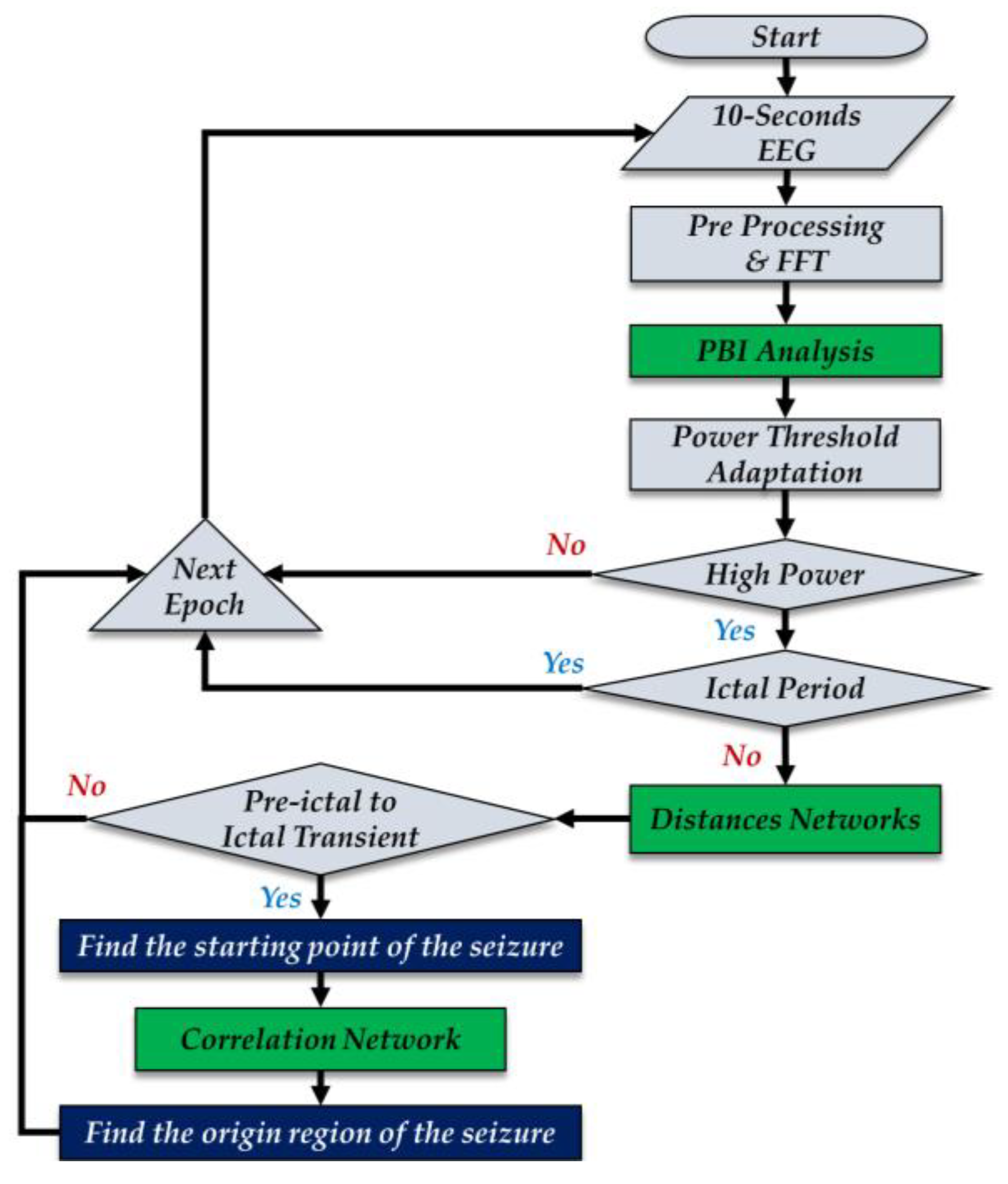
Figure 1 is a flowchart of the proposed algorithm. The main steps in the workflow are the computation of power in a band of interest (PBI), the calculation of distances in the network of electrodes (DN), and the computation of correlation within the network (CN). The EEG signals are divided into 10 s epochs with a 5 s overlap between epochs. The signals in each epoch are preprocessed to remove the DC offset and the 60 Hz line noise. These processed signals are decomposed into the frequency bands specified in Table 1 using the fast Fourier transform (FFT).
Previous studies, such as Adeli et al. [24], used all frequency bands when studying the EEG signals, while other studies, such as those of Shoeb and Guttag [25], used a limited frequency range (0.5–25 Hz). In the normal brain state, the power in the delta band has the largest variance [26]. The beta band activity corresponds to the performance of motor tasks and the performance of cognitive tasks with sensorimotor interactions [27]. Thus, the beta band activity varies based on the task in progress. Therefore, capturing the transition from the normal state to abnormal states (seizures in this case) is challenging if we use information from the delta and beta bands. Lee et al. [28], investigating seizures using electrocorticography (ECoG) or intracranial EEG, reported either rhythmic theta–alpha spike activity or rhythmic theta–alpha sinusoidal waves at seizure onset. Our hypothesis in this study is that theta–alpha activity will also provide an indication of seizure onset with scalp EEG. Hence, in this study we have used the activity in the theta–alpha band to compute the PBI measure.
Primarily due to historical reasons, such as the use of paper for recording EEG waveforms, clinical EEG interpretation generally relies on signals below 30 Hz. The advent of digital displays has brought about an interest in, and a utilization of, higher frequency components of the EEG signal. It has been noted [6,7,29] that high-frequency oscillations (HFOs) between 80 and 500 Hz contain spatial and temporal information about epileptic seizures. While most studies on HFOs are based on ECoGs it has been suggested that HFOs may also be useful for studying seizures using scalp EEG [7]. Unfortunately, there is significant contamination of the EEG signals with the electromyogram (EMG) between 20 to 300 Hz, and the level of contamination increases with increasing frequency [30]. However, new studies suggest that the use of HFOs with EEGs is also possible by filtering out or lessening the EMG contamination noises on EEG recordings [29]. Because of the existence of EMG coherence across EEG leads [31], it seems reasonable to assume that when we examine the difference between leads, the effect of this contamination will be reduced. In this study, because of the sampling frequency of the datasets used, the high gamma band is considered to be representative of the HFOs. Therefore, for measures of network connectivity which involve the distance between the nodes in the network, we use the spectral coefficients from the high gamma band.
2.1. Power in Band of Interest
One of the features used for distinguishing brain activity is the change in power in the EEG signal. This feature has been widely studied for differentiating between seizure and non-seizure EEG signals [23,32,33]. A significant rise in the magnitude of certain frequency components in the EEG signal can be a sign of a transition towards abnormal brain activity, such as the transition from a preictal to an ictal state. In the proposed algorithm, we measure this change in the following manner. For each lead, or channel, c, and epoch, t, the channel power, or the power at each electrode, (PE), in the frequency band of interest is computed as the sum of the squared magnitude of the appropriate FFT coefficient.
where are the FFT coefficients of the EEG signal from the channel c obtained during epoch t in the frequency band of interest, and n is the number of FFT coefficients in that band. The total power (P) during epoch t is then computed as the sum of the power in each band.
where K is the number of leads. As we are interested in the change in power, the power obtained using Equation (2) is normalized to get the value of the power in the band of interest (PBI) for epoch t as
The computed power in the current epoch is normalized by the background activity. The background activity is measured using the maximum and minimum power in the epochs from about 3 min to the current epoch to about 90 s prior to the current epoch. Each epoch overlaps the previous epoch by 5 s. Therefore, the variable j in Equation (3) is set to 17. Since neuronal activity differs between individuals, activity that may signal abnormal behavior in one individual may not do so in another individual. Therefore, we compute an adaptive threshold, as described in the following section, to determine the significance of the PBI value. If the PBI value for an epoch is greater than the adaptive threshold, we declared the current epoch to be a candidate for being in an ictal period.
2.2. Adaptive Threshold
Each individual’s brain activity is different. Therefore, we use an adaptive PBI threshold as opposed to a static threshold [34] to determine whether the activity in the epoch under consideration is abnormal. The adaptive threshold is calculated using the PBI values in three blocks of epochs:
- The first block consists of the epochs from the beginning of the record to the epoch terminating at 3 min prior to the epoch under consideration.
- The second block consists of the epochs from 3 min prior to the current epoch to 90 s (one and a half minutes) before the current epoch.
- The third block consists of the epochs from 90 s prior to the current epoch to the beginning of the current epoch.
These three blocks represent the background, recent, and current brain activities, respectively. We compute the average PBI values in each block denoted by PBI1, PBI2, and PBI3. The adaptive threshold (τ) is computed as a weighted average of these three values, further weighted by an adaptation coefficient (α), which can be used to adjust the sensitivity of the algorithm.
After 3 min from the beginning of a record, the adaptive threshold is adjusted for each epoch. In Equation (4), the weight of the first PBI block is two times higher than the second and third, as the average of the first PBI block carries more information about the background activity of the brain. The second and third blocks are equally important for capturing activity during transition, hence they are weighted equally.
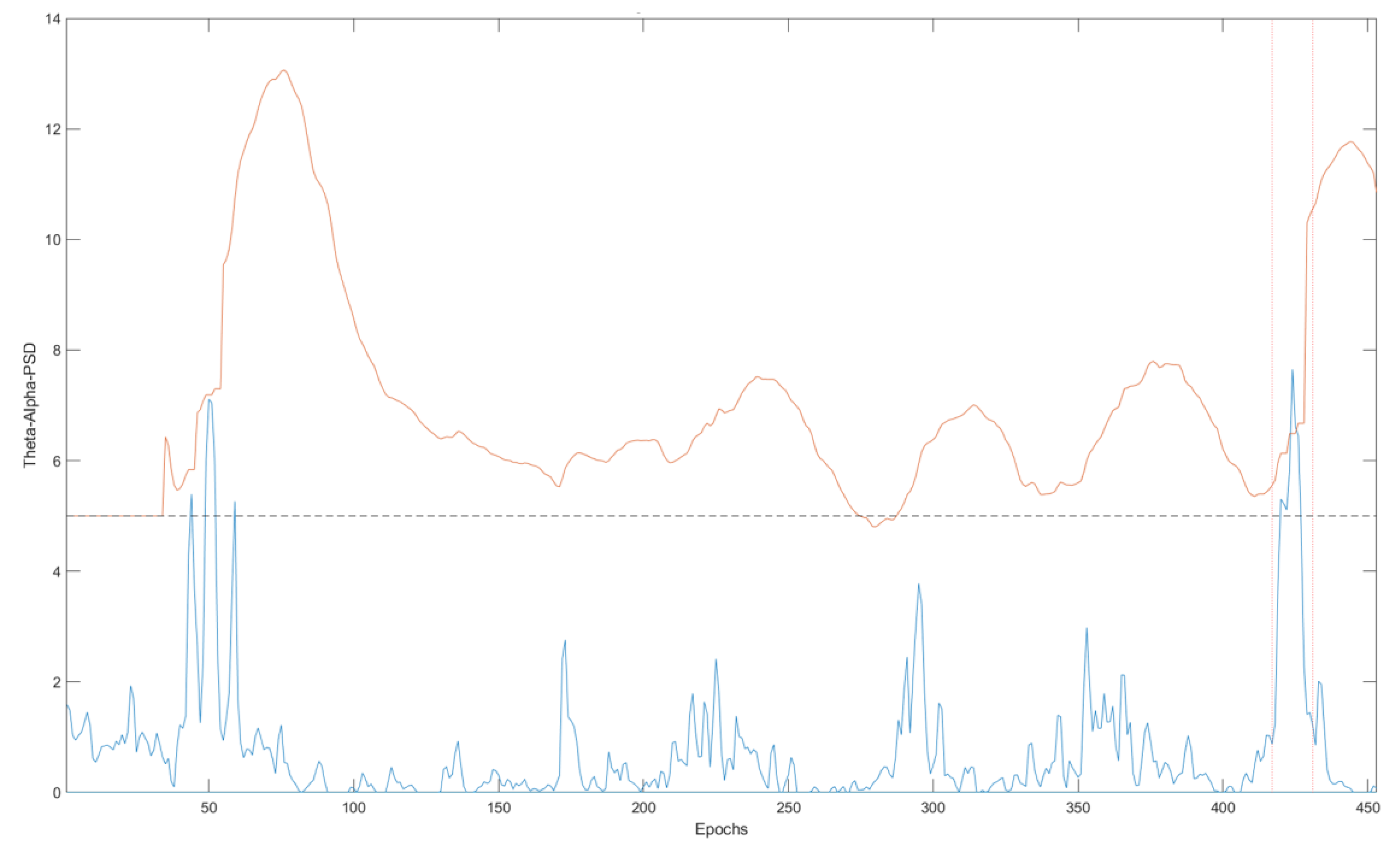
Figure 2 contains an example of the PBI values for a complete EEG record and the corresponding τ values for each epoch. The seizure period is marked by the red dashed line (between epoch 400 and epoch 450). If the threshold was set to a fixed default value (the black dashed line), there would be three events sensed as abnormal activities around the 50th epoch, however, the PBI is greater than the adaptive threshold (orange) only during the seizure periods. When the PBI is greater than the adaptive threshold, we declare the epoch to be a candidate for a seizure epoch. As described in the next section, we then verify that a seizure has indeed taken place by examining the network connectivity measures.
2.3. Distance Network
During the progression of a seizure, because of hypersynchronization, the similarity between the signals from neighboring EEG leads is expected to increase. We define a distance between two EEG leads, or channels, as the Euclidean distance between the FFT coefficients that correspond to the high gamma band. A matrix of size is generated where K is the number of channels and N is the number of FFT coefficients in the high gamma band. A distance matrix D is obtained by calculating the Euclidean distance between frequency components in a band for each pair of channels.
Assuming these distances reflect the synchronicity between the neuronal areas observed by electrode pairs, we expect to observe a close relation (lower distance) and a sudden increase in the closeness of channels during the preictal to ictal transient period. We define a normalized distance (DN) matrix
where Dmax, and Dmin are the maximum and minimum distances in the epoch, respectively. The normalized values lie between 0 and 1. A threshold of 0.1 is chosen to capture more than 90% similarity between a pair of electrodes. A pair of channels with a distance less than the threshold is assumed to be connected and an edge is created between the two nodes (EEG electrodes). Hypersynchronization during a seizure means that the number of connections in this network, which we call the distance network (DN), will increase as the seizure progresses. Therefore, a measure of hypersynchronization in a region of the brain is the number of possible connections which are activated. Letting R be the number of pairs of channels in a particular region with distance less than the threshold, and letting T be the total number of pairs of channels in the region, then we define the connection ratio CR as
If there are n channels in a region, the total number of possible connections in a region, T, is The EEG channels are divided into eight regions: right and left hemispheres, frontal, temporal, parietal, and occipital lobes, in addition to the central region and the general region, which consists of all of the EEG channels.
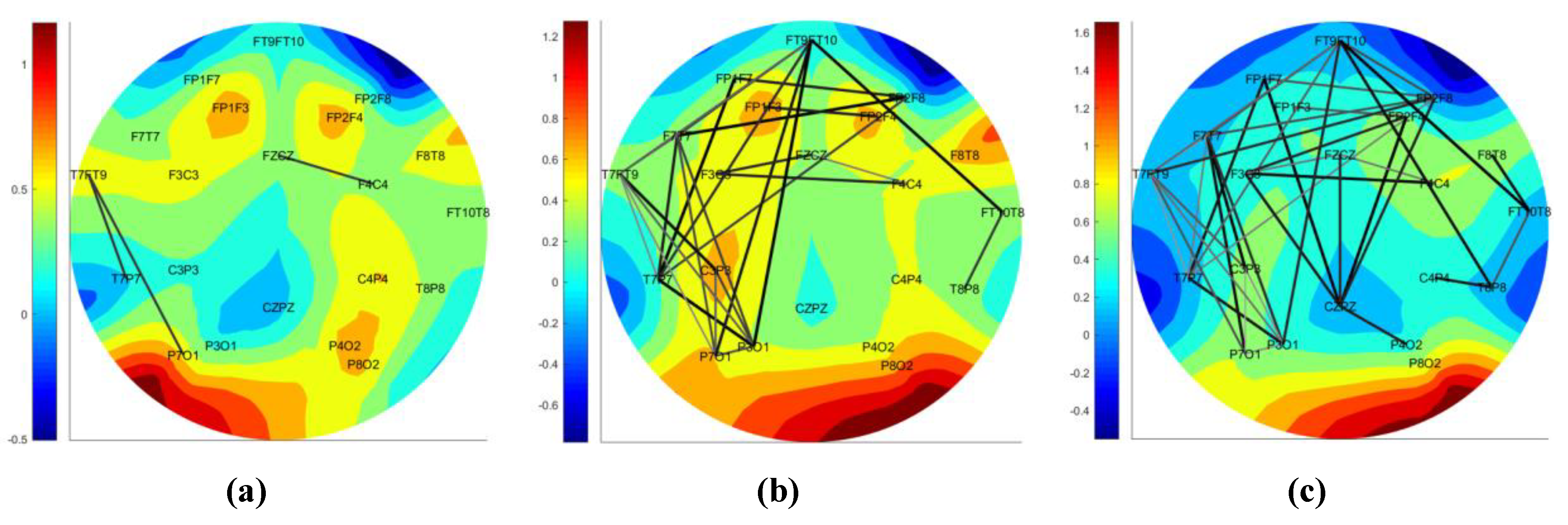
The connection ratio is evaluated after sensing an abnormality activity using the PBI method. To determine a transition from a preictal to ictal period, the DN is studied in the high gamma band. An example of this increase in the connection ratio during transition from preictal to ictal is shown in Figure 3. Figure 3a shows the DN at an epoch before a seizure start, and Figure 3b,c shows the increase in connections as the seizure progresses. The connection ratio in a region should be greater than 0.2 in order to declare a focal seizure in a region. A generalized seizure covers more than a focal seizure. Note that we only compute the connection ratio if the PBI measure indicates the possibility of a seizure. The background color of the DN schematic, displayed in Figure 3a–c, shows the relative power of the channels, with darker red regions indicating higher brain activity.
The DNs indicate the increase in closeness and model a spreading seizure in the brain. However, this approach is not capable of locating the origin of a seizure. For locating the focus of a seizure, the CN is generated.
2.4. Correlation Network
The PBI and DN measures are used to detect the presence of a seizure. On the basis of the neuronal hypersynchronization during the ictal period [5,6], another network of EEG channels similar to DN is generated for locating the origin of a seizure. In this network, we use correlation between the channels to determine connectivity.
While correlation between EEG channels is not restricted to the ictal period, assuming that the correlation of a pair of channels reflects their synchronization, we expect to observe a higher correlation among synchronized electrodes in a seizure region (and neighboring regions) during an ictal period.
After pre-processing and filtering an epoch of an EEG signal into a frequency band, a (K = number of electrodes) matrix of Pearson correlations is generated by calculating correlation coefficients of pairs of channels. The Pearson correlation between channel A and B can be calculated by Equation (7).
where N, represents the number of FFT frequency components, µA and µB represent the averages of FFT components in channels A and B, and represent the standard deviations of the spectral components in channels A and B. The closeness (C) factor of channels A and B is defined by Equation (8).
where (t,A) and (t,B) are the normalized power obtained using Equation (1) normalized by the maximum power of a channel in that epoch. Therefore, (t,A) and (t,B) are in the range of [0, 1]. Channel synchronization should have more impact on their closeness (C). A high correlation coefficient of a pair of channels indicates a possible hypersynchronization of channels. In this formula, the correlation coefficient is raised to the second power while the average channel power ((t,A) +(t,B))/2 is raised to the third power. As each of these terms has a value less than one, this accentuates the effect of the correlation coefficient with respect to the average power in Equation (8). To define a connection in a correlation network, a threshold of 0.85 is used: Two electrodes are connected if their closeness (C) factor is greater than 0.85. Connected electrodes generate a CN. The edges of the CN are normalized by the maximum edge (with maximum closeness (C)) of the same network. The normalized edges determine the relative degree of closeness of two channels. Figure 4 demonstrates a CN generated at the beginning epoch of a seizure. The higher the closeness of electrodes, the darker and thicker the connections. The strength of connections in a brain region is defined as the average of the two strongest (closest) connections in the corresponding region.
The type and the focus of the seizure can be identified by the CNs. If a seizure spread rapidly in brain regions and covers most of the brain at the beginning of the seizure, it is considered to be a generalized seizure; otherwise, it is most likely to be a focal seizure. The rapid spreading of the seizure at the beginning is captured by the number of connected edges. If more than half (60%) of the electrode pairs are connected at the beginning of a seizure, the seizure is determined to be a generalized seizure; otherwise, it is considered a focal seizure.
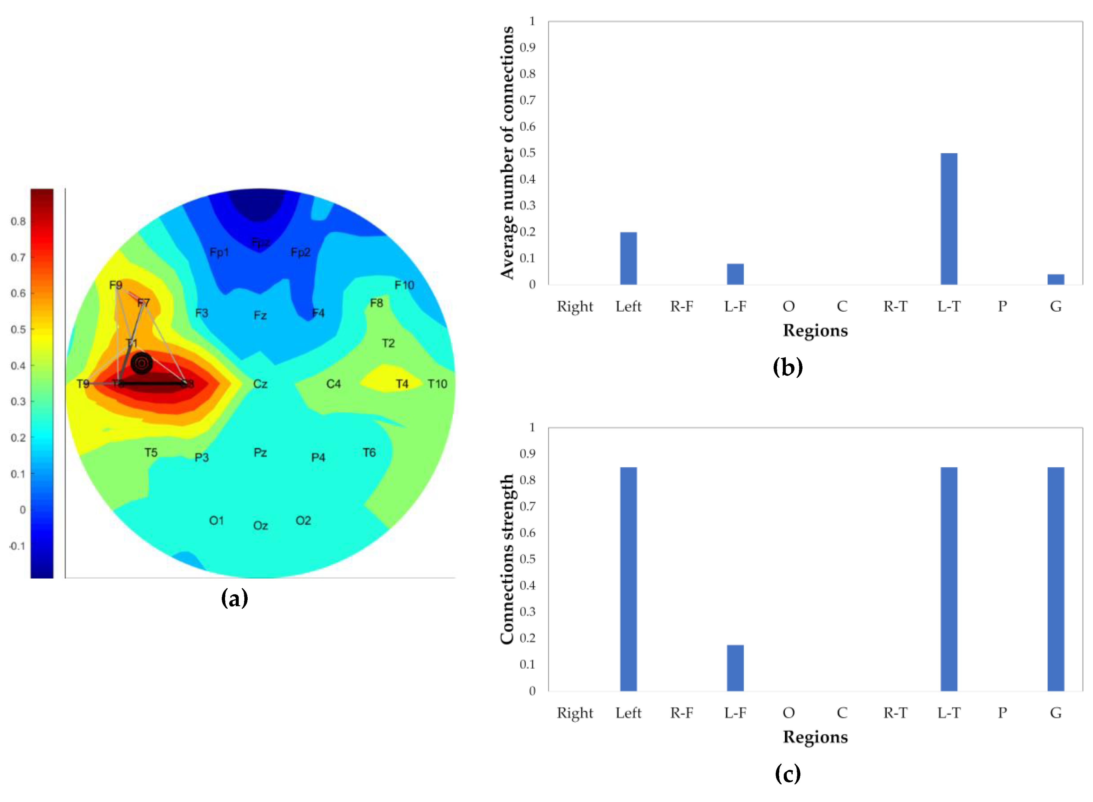
To locate the origin of a seizure, the 10-second epoch in which the seizure is determined to have begun—which has been determined by the PBI and DN methods—is divided into 2-second sub-epochs with a 1 s overlap between sub-epochs, resulting in nine 2-second sub-epochs. The CN is generated for all 2-second sub-epochs of the event. The connection ratio of CN in the high gamma band in brain regions (R-F (right-frontal), L-F (left-frontal), occipital, central, R-T (right-temporal), L-T (left-temporal), parietal) is calculated for each sub-epoch (Figure 4b). The first sub-epoch with a region connectivity more than 40% is defined as the start of the seizure. If none of the sub-epochs pass this criterion, the first sub-epoch (which is the first 2 s of the epoch containing the beginning of the seizure) is assumed to contain the seizure origin. As mentioned before, seizures are assumed to result in increased similarity between neighboring electrodes. Therefore, to locate the seizure origin, two CN parameters of the chosen sub-epoch, the connection ratio (indication of the malfunction of neuronal inhibition and excitation activity) and strength of connections (an indication of the hypersynchronization of neighboring neuronal regions) are considered simultaneously. This is done by computing the product of these values. The region with the maximum product of these two parameters is picked as the origin of the seizure. For instance, in Figure 4, the seizure is located in the L-T lobe. Also, a finer localization is marked on the CN schematic calculated by the three electrode coordinates of the two strongest connections in the defined seizure origin region. The centroid of the three electrodes is defined as the seizure origin and visualized by filled circles. The marked origin of the seizure in Figure 4a is located in the L-T region, closer to the electrodes with higher relative power. As mentioned in Section 2.3, the background color of the CN, as well as the DN network, represents the relative power of channels.
2.5. Dataset
Two datasets were used for evaluating the performance of the proposed approach. The Physionet dataset, provided by the Children’s Hospital Boston (CHB-MIT) [35], is comprised of 980 h of EEG records, obtained from 24 patients with a total of 185 seizure attacks and is used for the detection of seizures. Since the CHB-MIT dataset does not provide localization information about the seven seizures, a second dataset obtained from the Karunya University EEG database [36] was used, which contains 10 s EEG seizure activity. This dataset was used to evaluate localization performance. Both datasets are publicly available. Table 2 contains the descriptions for each patient obtained by the CHB-MIT dataset, sampled at 256 Hz, and includes the length of the EEG signals, the number of seizures, and the average seizure durations. The Karunya dataset also has a sampling rate of 256 Hz, but is additionally filtered through an analog bandpass filter with cutoff frequencies of 0.01 Hz and 100 Hz. This dataset contains a total of 175 10-second EEG seizure sequences obtained from patients with an age range spanning from 1 to 107 (33 ± 22) years old, involving 88 generalized and 87 focal seizures.
3. Results
The performance of the proposed algorithm was evaluated for temporal seizure detection by applying it to the CHB-MIT dataset. Most studies that have used this dataset have focused on the ages between 4 and 21 years old, which is what we did also. Therefore, patients 4, 6, 10, 12, and 13 were excluded from the seizure detection algorithm and further analyses. Although patient 8 was 3.5 years old, their EEG recordings were included in the evaluation. Additionally, for the spatial seizure detection evaluation, the algorithm was also applied to the Karunya dataset.
The temporal performance of the proposed algorithm was evaluated using two metrics: true positive rate (TPR) or sensitivity (() × 100), and false positives per hour (FPH). Furthermore, detection latency was also calculated for the detected seizures. Table 3 summarizes the results for each patient individually.
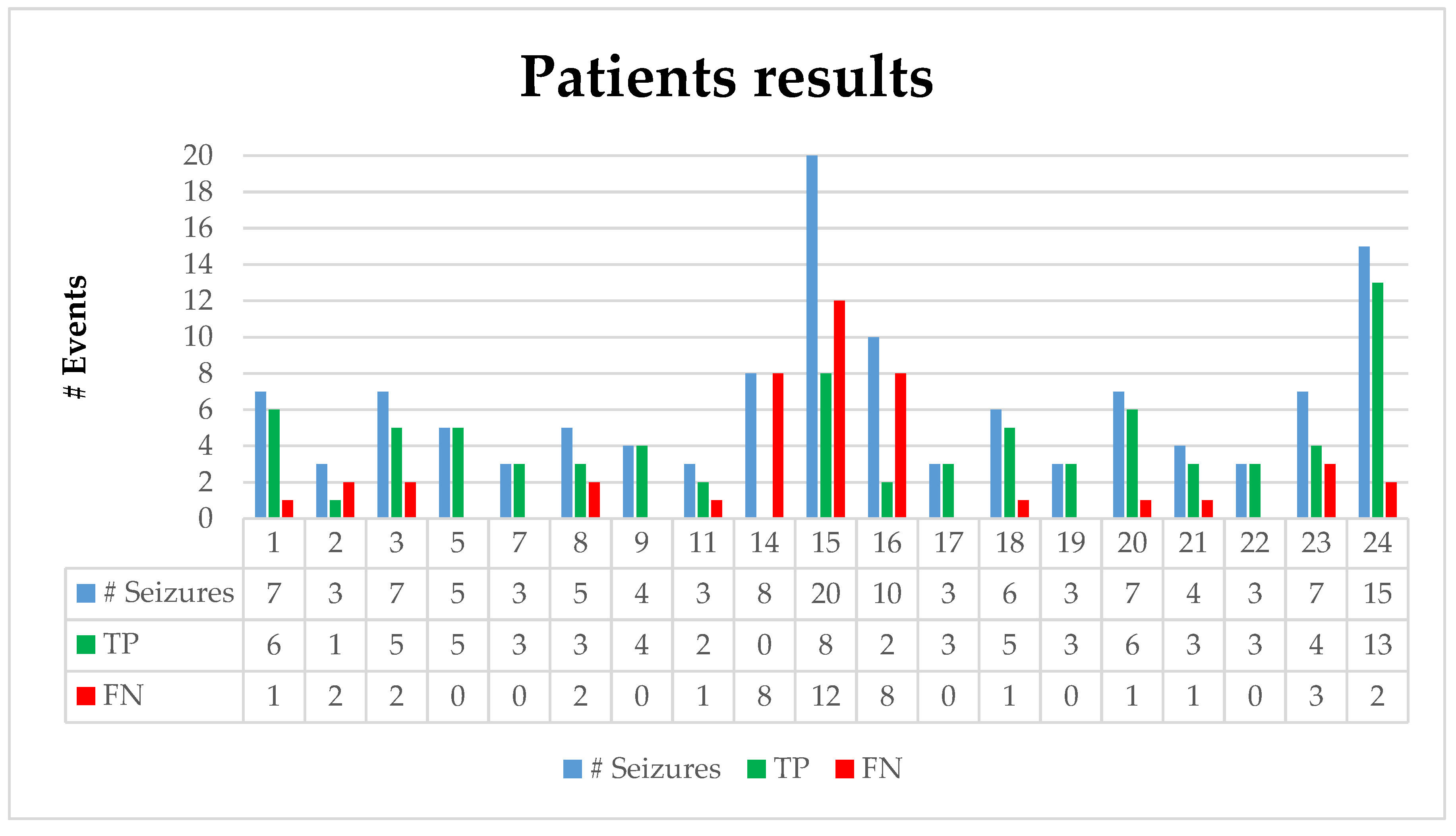
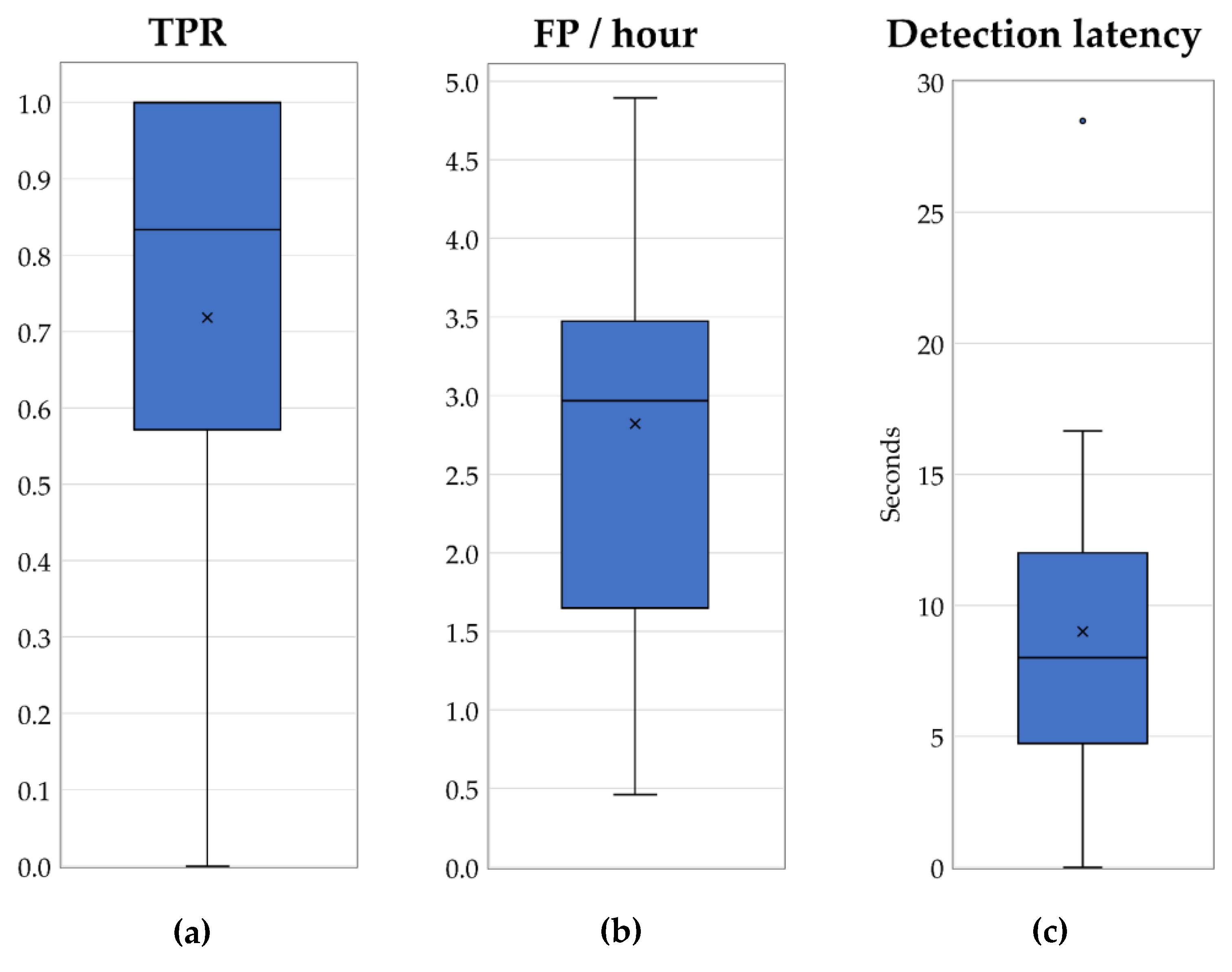
Figure 5 illustrates the number of seizures, true positives (TPs) (number of correctly predicted seizures), and false negatives (FNs) (number of missed true seizures) for each individual patient. As mentioned in Section 2.1, PBI normalization requires at least 3 min of EEG recording; therefore, the events prior to the first 3 min of an EEG record cannot be evaluated. Patients 17 and 24 had one seizure activity which ended before the third minute of the recording; hence, those events were removed from the dataset. Patient 2 had seizure activity between 130–212 s of the recording. Although the activity started prior to the third minute of the recording, our algorithm detected it at the 180th second, which affected the detection latency period. Therefore, the beginning of the seizure is assumed to be at that time to fix the negative effect on the detection latency; otherwise, it would contain a 50 s latency. The adaptive coefficient (α) was set to 5. The boxplots in Figure 6a–c represent the overall performance of the proposed algorithm and illustrate the median, outliers, and ranges of the performances. Table 4, which summarizes the detailed results of Table 3, contains the overall temporal performances of the proposed approach.
The evaluation of the spatial performance of the proposed algorithm was based on the concurrence of the labeled seizure origins in the Karuniya dataset with the localization results of the algorithm. Table 5 summarizes the spatial performance of the proposed approach on the Karuniya dataset. Seizures of generalized or focal types were analyzed. Additionally, if the localized seizure lobe in the right, left, and central regions concurred with the focus of the seizure annotated by the dataset, the localization was counted as a correct localization. The second and third columns in Table 5 contain the total number of the EEG records and the ones that were correctly localized. The last column shows the sensitivity (TPR) measures for seizure type determination and region localization.
4. Discussion
Detecting seizures is a challenging problem, and a real-time seizure detection algorithm is even more challenging. Previous studies have shown a promising performance for detecting seizures, as shown in Table 6. However, those algorithms require a large amount of training on the data from previous seizures (patient-specific methods) or training on EEG signals of different seizure and non-seizure periods (seizure-specific methods). For instance, Shoeb [20] and Nasehi and Pourghassem [37] obtained a better sensitivity value (96% and 98%, respectively) than the TPR reported in this study (mean TPR = 72%, median TPR = 83%). However, their approaches were trained and tested on a specific patient.
Although non-patient-specific approaches are more amenable to generalization compared to patient-specific methods, they require a huge amount of the EEG data for training their classifiers. Saab and Gotman [48] used a training set which contained 652 h EEG data including 126 clinical seizures from 28 patients, and the Kuhlmann [50] training set consisted of 367 h of EEG signals, which contained 58 clinical seizures from 14 patients. Despite the size of the training dataset for these two studies, the non-trained proposed method has generally outperformed them.
The overall performance of the proposed method was negatively affected by three patients—14, 15, and 16. Excluding these outliers enhances the overall TPR (mean TPR = 81.5%, median TPR = 85.7%). The main reason for the poor performance of the algorithm on these patients was an excessive level of artifacts. The EEG signals from patients 14 and 15 contained significant artifacts in the recordings and would require an enhanced preprocessing method to be able to differentiate the activities. The seizures for patient 16 lasted an average of only 8.4 s, which was less than the length of the epoch of the proposed system. Only one seizure lasted more than 10 s (14 s). It is hoped that by decreasing the epoch size, these types of short seizures attacks will be detectable.
Compared to previous studies using computationally expensive classifiers, such as neural networks and PSO, the proposed algorithm is time-efficient and cost-effective. Table 7 contains the average times required to compute the main functions in milliseconds. The computation times were calculated for an implementation in MATLAB R2017b with Intel Core i7-6700 CPU @ 4.00 GHz with 32 GB RAM. The FFT, PBI, and threshold adaptation functions are computed for every 10 second epoch. The most computationally expensive part of the proposed algorithm is the generation of the CN. On average, these networks needed to be calculated three times per hour (FPH of 2.9), which requires approximately 25 ms per hour. Zabihi et al., [44] implemented their proposed method on the same dataset using MATLAB version R2014b with a 3.4 GHz processor and 16 GB RAM. The time required for feature extraction for one second of one EEG channel was reported as 2.6 ms. For an hour of EEG analysis on one channel, the time required for feature extraction with linear discriminant analysis (LDA) classification is about 9.6 s. Supratak et al. [41] implemented their algorithm in MATLAB with a 3.4 GHz machine with 16.0 GB RAM. The reported training time varied from 2 to 5 h, depending on the amount of training for each patient, and the computation time for seizure detection was reported as ~10 ms for each 1-second EEG segment. This translates to about 36 s for an hour of EEG activity without considering the amount of time devoted to training. In contrast, for the proposed algorithm, the average computation time for analysis of an hour worth of EEG data for all channels is about 2.2 s.
In addition to detecting a seizure occurrence, this study proposes a simultaneous localization of the seizure. EEG localization methods have lower spatial resolution compared to the other methods, such as MEG or fMRI, but the portability of EEG devices makes them a popular approach for some cases such as long-term monitoring (LTM) with wearable EEG devices for post-surgery seizure monitoring or monitoring the effect of antiepileptic drugs (AEDs) on a patient. Table 5 contains the localization performance of 175 EEG seizure sequences from the Karuniya dataset. The underlying hypothesis for locating the origin of a seizure using the proposed algorithm is to capture the seizure characteristic at the beginning of a seizure and localize it. The Karuniya EEG records are 10 s segments of a seizure, which could be at the beginning, middle, or last ten seconds of an ictal period. The localization performance would be enhanced if the EEG records all contained the beginning of seizures. The Karuniya patients were diagnosed with a variety of neurological disorders, such as dementia, and the dataset was not focused on epileptic seizures. Other disorders should be studied separately for localization because of their unique characteristic of neuronal activities. In addition to the low-frequency resolution of the Karuniya dataset (filtered by an analog bandpass filter with cutoff frequencies of 0.01 Hz and 100 Hz) which reduces the CN efficiency, the proposed method demonstrated acceptable performance on defining the type of seizures and localization of brain lobes rather than the hemispheres. Furthermore, this algorithm is applicable on different EEG electrode montages, such as the ipsilateral referential montage (Karuniya dataset) and the bipolar montage (CHB-MIT dataset).
5. Conclusions and Future Work
The proposed method is a tunable non-patient-specific, non-seizure-specific method that can detect a seizure period and simultaneously locate the origin of the seizure on the scalp. It has a better average detection latency (8 s) and comparable median TPR (83%) and acceptable FPH (2.9 FP/hour), when compared to previous studies, which are much more computationally intense, and are less practical for many applications. To further improve the algorithm, in particular the seizure localization, we plan to add independent component analysis (ICA) and surface Laplacian [52] to the preprocessing method for suppressing EMG contamination. One of the major challenges we faced was access to a public dataset which provides temporal and spatial information simultaneously. In collaboration with neurologists at Creighton University, we plan to build a comprehensive and well-annotated publicly available dataset which will contain both temporal and spatial information about the EEG signals. Finally, in addition to using this approach for LTM clinical trials, we hope to implement this algorithm in a wearable portable device that can be deployed to resource-constrained areas for detecting and monitoring patients with epilepsy.
Author Contributions
Conceptualization, A.M., S.S., and K.S.; methodology, A.M. and K.S.; software, A.M.; writing—original draft preparation, A.M.; writing—review and editing, A.M. and K.S.; visualization, A.M.; supervision, K.S. and S.S.
Funding
This research received no external funding.
Acknowledgments
We would like to thank the anonymous reviewers for their very constructive comments and to Patricia Worster for her careful reading and editing of the manuscript.
Conflicts of Interest
The authors declare no conflict of interest.
References
- Hirtz, D.; Thurman, D.J.; Gwinn-Hardy, K.; Mohamed, M.; Chaudhuri, A.R.; Zalutsky, R. How common are the common neurologic disorders? Neurology 2007, 68, 326–337. [Google Scholar] [CrossRef]
- Fisher, R.S.; Scharfman, H.E. How can we identify ictal and interictal abnormal activity? In Issues in Clinical Epileptology: A View from the Bench. Springer Netherlands. Adv. Exp. Med. Boil. 2014, 813, 3–23. [Google Scholar]
- Shorvon, S.; Tomson, T. Sudden unexpected death in epilepsy. Lancet 2011, 378, 2028–2038. [Google Scholar] [CrossRef]
- Staley, K. Molecular mechanisms of epilepsy. Nat. Neurosc. 2015, 18, 367–372. [Google Scholar] [CrossRef] [Green Version]
- Paz, J.T.; Huguenard, J.R. Microcircuits and their interactions in epilepsy: Is the focus out of focus? Nat. Neurosci. 2015, 18, 351–359. [Google Scholar] [CrossRef] [PubMed]
- Jiruska, P.; De Curtis, M.; Jefferys, J.G.; Schevon, C.A.; Schiff, S.J.; Schindler, K. Synchronization and desynchronization in epilepsy: Controversies and hypotheses. J. Physiol. 2013, 591, 787–797. [Google Scholar] [CrossRef] [PubMed]
- Gotman, J. High frequency oscillations: The new EEG frontier? Epilepsia 2010, 51, 63–65. [Google Scholar] [CrossRef] [Green Version]
- Gaitatzis, A.; Johnson, L.A.; Chadwick, W.D.; Shorvon, D.S.; Sander, W.J. Life expectancy in people with newly diagnosed epilepsy. Brain 2004, 127, 2427–2432. [Google Scholar] [CrossRef] [Green Version]
- Gogtay, N.; Giedd, J.N.; Lusk, L.; Hayashi, K.M.; Greenstein, D.; Vaituzis, A.C.; Nugent, T.F.; Herman, D.H.; Clasen, L.S.; Toga, A.W.; et al. Dynamic mapping of human cortical development during childhood through early adulthood. Proc. Natl. Acad. Sci. USA 2004, 101, 8174–8179. [Google Scholar] [CrossRef] [Green Version]
- Wierenga, L.; Langen, M.; Ambrosino, S.; van Dijk, S.; Oranje, B.; Durston, S. Typical development of basal ganglia, hippocampus, amygdala and cerebellum from age 7 to 24. Neuroimage 2014, 96, 67–72. [Google Scholar] [CrossRef]
- Camfield, P.; Camfield, C.; Busiah, K.; Cohen, D.; Pack, A.; Nabbout, R. The transition from pediatric to adult care for youth with epilepsy: Basic biological, sociological, and psychological issues. Epilepsy Behav. 2017, 69, 170–176. [Google Scholar] [CrossRef] [PubMed]
- Fuhrmann, D.; Knoll, L.J.; Blakemore, S.J. Adolescence as a sensitive period of brain development. Trends Cogni. Sci. 2015, 19, 558–566. [Google Scholar] [CrossRef] [PubMed]
- WHO. Available online: https://www.who.int/en/news-room/fact-sheets/detail/epilepsy (accessed on 20 June 2019).
- De Boer, H.M.; Mula, M.; Sander, J.W. The global burden and stigma of epilepsy. Epilepsy Behave. 2008, 12, 540–546. [Google Scholar] [CrossRef] [PubMed]
- Dall, T.M.; Storm, M.V.; Chakrabarti, R.; Drogan, O.; Keran, C.M.; Donofrio, P.D.; Vidic, T.R. Supply and demand analysis of the current and future US neurology workforce. Neurology 2013, 81, 470–478. [Google Scholar] [CrossRef] [Green Version]
- Rommens, N.; Geertsema, E.; Holleboom, L.J.; Cox, F.; Visser, G. Improving staff response to seizures on the epilepsy monitoring unit with online EEG seizure detection algorithms. Epilepsy Behav. 2018, 84, 99–104. [Google Scholar] [CrossRef] [PubMed]
- Proctor, C.M.; Slézia, A.; Kaszas, A.; Ghestem, A.; Del Agua, I.; Pappa, A.M.; Bernard, C.; Williamson, A.; Malliaras, G.G. Malliaras. Electrophoretic drug delivery for seizure control. Sci. Adv. 2018, 4, eaau1291. [Google Scholar] [CrossRef] [PubMed]
- Jensen, M.P.; Liljenquist, K.S.; Bocell, F.; Gammaitoni, A.R.; Aron, C.R.; Galer, B.S.; Amtmann, D. Life impact of caregiving for severe childhood epilepsy: Results of expert panels and caregiver focus groups. Epilepsy Behav. 2017, 74, 135–143. [Google Scholar] [CrossRef] [PubMed]
- Bergey, G.K. Neurostimulation in the treatment of epilepsy. Exp. Neurol. 2013, 244, 87–95. [Google Scholar] [CrossRef] [PubMed]
- Shoeb, A.H. Application of Machine Learning to Epileptic Seizure Onset Detection and Treatment. Ph.D. Thesis, Massachusetts Institute of Technology, Cambridge, UK, 2009. [Google Scholar]
- Shoeb, A.; Edwards, H.; Connolly, J.; Bourgeois, B.; Treves, S.T.; Guttag, J. Patient-specific seizure onset detection. Epilepsy Behav. 2004, 4, 483–498. [Google Scholar] [CrossRef] [PubMed]
- Meier, R.; Dittrich, H.; Schulze-Bonhage, A.; Aertsen, A. Detecting epileptic seizures in long-term human EEG: A new approach to automatic online and real-time detection and classification of polymorphic seizure patterns. J. Clin. Neurophysiol. 2008, 25, 119–131. [Google Scholar] [CrossRef]
- Tzallas, A.T.; Tsipouras, M.G.; Fotiadis, D.I. Epileptic seizure detection in EEGs using time–frequency analysis. IEEE Trans. Inf. Technol. Biomed. 2009, 13, 703–710. [Google Scholar] [CrossRef] [PubMed]
- Adeli, H.; Ghosh-Dastidar, S.; Dadmehr, N. A wavelet-chaos methodology for analysis of EEGs and EEG subbands to detect seizure and epilepsy. IEEE Trans. Biomed. Eng. 2007, 54, 205–211. [Google Scholar] [CrossRef] [PubMed]
- Shoeb, A.H.; John, V.G. Application of machine learning to epileptic seizure detection. In Proceedings of the 27th International Conference on Machine Learning (ICML-10), Haifa, Israel, 21–24 June 2010; pp. 975–982. [Google Scholar]
- Capitán, M.M.; Cámpora, N.; Kochen, S.; Samengo, I. Principal Component Analysis for seizure characterization in EEG signals. arXiv 1902, arXiv:1902.112361902. [Google Scholar]
- Herrmann, C.S.; Strüber, D.; Helfrich, R.F.; Engel, A.K. EEG oscillations: From correlation to causality. Int. J. Psychophysiol. 2016, 103, 12–21. [Google Scholar] [CrossRef] [PubMed]
- Lee, S.A.; Spencer, D.D.; Spencer, S.S. Intracranial EEG seizure-onset patterns in neocortical epilepsy. Epilepsia 2000, 41, 297–307. [Google Scholar] [CrossRef] [PubMed]
- Jacobs, J.; Staba, R.; Asano, E.; Otsubo, H.; Wu, J.Y.; Zijlmans, M.; Mohamed, I.; Kahane, P.; Dubeau, F.; Navarro, V.; et al. High-frequency oscillations (HFOs) in clinical epilepsy. Prog. Neurobiol. 2012, 98, 302–315. [Google Scholar] [CrossRef] [Green Version]
- Muthukumaraswamy, S. High-frequency brain activity and muscle artifacts in MEG/EEG: A review and recommendations. Front. Hum. Neurosci. 2013, 7, 138. [Google Scholar] [CrossRef]
- Pope, K.J.; Fitzgibbon, S.P.; Lewis, T.W.; Whitham, E.M.; Willoughby, J.O. Relation of Gamma Oscillation in Scalp Recordings to Muscular Activity. Brain Topogr. 2009, 22, 13–17. [Google Scholar] [CrossRef]
- Polat, K.; Güneş, S. Classification of epileptiform EEG using a hybrid system based on decision tree classifier and fast Fourier transform. Appl. Math. Comput. 2007, 187, 1017–1026. [Google Scholar] [CrossRef]
- Alkan, A.; Kiymik, M.K. Comparison of AR and Welch methods in epileptic seizure detection. J. Med. Syst. 2006, 30, 413–419. [Google Scholar] [CrossRef]
- Mansouri, A.; Singh, S.; Sayood, K. Hierarchal online temporal and spatial EEG seizure detection. In Proceedings of the 2017 IEEE International Conference on Electro Information Technology (EIT), Lincoln, NE, USA, 14–17 May 2017. [Google Scholar]
- Goldberger, A.L.; Amaral, L.A.; Glass, L.; Hausdorff, J.M.; Ivanov, P.C.; Mark, R.G.; Stanley, H.E. Physiobank, physiotoolkit, and physionet. Circulation 2000, 101, e215–e220. [Google Scholar] [CrossRef] [PubMed]
- Selvaraj, T.G.; Ramasamy, B.; Jeyaraj, S.J.; Suviseshamuthu, E.S. EEG database of seizure disorders for experts and application developers. Clin. EEG Neurosci. 2014, 45, 304–309. [Google Scholar] [CrossRef] [PubMed]
- Nasehi, S.; Pourghassem, H. Patient-specific epileptic seizure onset detection algorithm based on spectral features and IPSONN classifier. In Proceedings of the 3rd International Conference on Communication Systems and Network Technologies (CSNT ‘13), IEEE, Gwalior, India, 6–8 April 2013; pp. 186–190. [Google Scholar]
- Zandi, A.S.; Javidan, M.; Dumont, G.A.; Tafreshi, R. Automated real-time epileptic seizure detection in scalp EEG recordings using an algorithm based on wavelet packet transform. IEEE Trans. Biomed. Eng. 2010, 57, 1639–1651. [Google Scholar] [CrossRef] [PubMed]
- Khan, Y.U.; Rafiuddin, N.; Farooq, O. Automated seizure detection in scalp EEG using multiple wavelet scales. In Proceedings of the 2012 IEEE International Conference on Signal Processing, Computing and Control, Solan, HP, India, 15–17 March 2012; pp. 1–5. [Google Scholar]
- Hunyadi, B.; Signoretto, M.; Van Paesschen, W.; Suykens, J.A.; Van Huffel, S.; De Vos, M. Incorporating structural information from the multichannel EEG improves patient-specific seizure detection. Clin. Neurophysiol. 2012, 123, 2352–2361. [Google Scholar] [CrossRef] [PubMed]
- Supratak, A.; Li, L.; Guo, Y. Feature extraction with stacked autoencoders for epileptic seizure detection. In Proceedings of the 2014 36th Annual International Conference of the IEEE Engineering in Medicine and Biology Society, Chicago, Il, USA, 26–30 August 2014; pp. 4184–4187. [Google Scholar]
- Kiranyaz, S.; Ince, T.; Zabihi, M.; Ince, D. Automated patient-specific classification of long-term electroencephalography. J. Biomed. Inform. 2014, 49, 16–31. [Google Scholar] [CrossRef]
- Samiee, K.; Kiranyaz, S.; Gabbouj, M.; Saramäki, T. Long-term epileptic EEG classification via 2D mapping and textural features. Expert Syst. Appl. 2015, 42, 7175–7185. [Google Scholar] [CrossRef]
- Zabihi, M.; Kiranyaz, S.; Rad, A.B.; Katsaggelos, A.K.; Gabbouj, M.; Ince, T. Analysis of high-dimensional phase space via Poincaré section for patient-specific seizure detection. IEEE Trans. Neural Syst. Rehabil. Eng. 2015, 24, 386–398. [Google Scholar] [CrossRef]
- Webber, W.R.S.; Lesser, R.P.; Richardson, R.T.; Wilson, K. An approach to seizure detection using an artificial neural network (ANN). Electroencephalogr. Clin. Neurophysiol. 1996, 98, 250–272. [Google Scholar] [CrossRef]
- Gabor, A.J. Seizure detection using a self-organizing neural network: Validation and comparison with other detection strategies. Electroencephalogr. Clin. Neurophysiol. 1998, 107, 27–32. [Google Scholar] [CrossRef]
- Wilson, S.B.; Scheuer, M.L.; Emerson, R.G.; Gabor, A.J. Seizure detection: Evaluation of the Reveal algorithm. Clin. Neurophysiol. 2004, 115, 2280–2291. [Google Scholar] [CrossRef]
- Saab, M.E.; Gotman, J. A system to detect the onset of epileptic seizures in scalp EEG. Clin. Neurophysiol. 2005, 116, 427–442. [Google Scholar] [CrossRef] [PubMed]
- Aarabi, A.; Wallois, F.; Grebe, R. Automated neonatal seizure detection: A multistage classification system through feature selection based on relevance and redundancy analysis. Clin. Neurophysiol. 2006, 117, 328–340. [Google Scholar] [CrossRef] [PubMed]
- Kuhlmann, L.; Burkitt, A.N.; Cook, M.J.; Fuller, K.; Grayden, D.B.; Seiderer, L.; Mareels, I.M. Seizure detection using seizure probability estimation: Comparison of features used to detect seizures. Ann. Biomed. Eng. 2009, 37, 2129–2145. [Google Scholar] [CrossRef] [PubMed]
- Fürbass, F.; Ossenblok, P.; Hartmann, M.; Perko, H.; Skupch, A.M.; Lindinger, G.; Elezi, L.; Pataraia, E.; Colon, A.J.; Baumgartner, C.; et al. Prospective multi-center study of an automatic online seizure detection system for epilepsy monitoring units. Clin. Neurophysiol. 2015, 126, 1124–1131. [Google Scholar] [CrossRef] [PubMed]
- Fitzgibbon, S.P.; DeLosAngeles, D.; Lewis, T.W.; Powers, D.M.; Whitham, E.M.; Willoughby, J.O.; Pope, K.J. Surface Laplacian of scalp electrical signals and independent component analysis resolve EMG contamination of electroencephalogram. Int. J. Psychophysiol. 2015, 97, 277–284. [Google Scholar] [CrossRef] [PubMed]
Figure 1.
Algorithm flowchart. EEG = electroencephalography, FFT = fast Fourier transform, PBI = power in a band of interest.
Figure 1.
Algorithm flowchart. EEG = electroencephalography, FFT = fast Fourier transform, PBI = power in a band of interest.

Figure 2.
An example of PBI and the dynamic PBI threshold. The blue and orange lines illustrate the PBI for each epoch and the PBI dynamic threshold, respectively.
Figure 2.
An example of PBI and the dynamic PBI threshold. The blue and orange lines illustrate the PBI for each epoch and the PBI dynamic threshold, respectively.

Figure 3.
The transition of the distance network (DN) from preictal to ictal. DN networks of (a) an epoch before the seizure, (b) beginning of the seizure, and (c) an epoch after the seizure start.
Figure 3.
The transition of the distance network (DN) from preictal to ictal. DN networks of (a) an epoch before the seizure, (b) beginning of the seizure, and (c) an epoch after the seizure start.

Figure 4.
Correlation within the network (CN) example at the beginning of a seizure; (a) CN contains connection, marked target of the seizure origin, and colored-background by the normalized power of the channels; (b) average number of connections in each region (right, left, right-frontal (R-F), left-frontal (L-F), occipital, central, right-temporal (R-T), left-temporal (L-T), parietal, general); and (c) strength of connection in each region.

Figure 5.
Results of the CHB-MIT dataset contains the number of seizures, the true positives (TP), and false positives (FP) for each patient.
Figure 5.
Results of the CHB-MIT dataset contains the number of seizures, the true positives (TP), and false positives (FP) for each patient.

Figure 6.
Temporal performance of the proposed algorithm: (a) TPR, (b) FP/hour, and (c) detection latency.
Figure 6.
Temporal performance of the proposed algorithm: (a) TPR, (b) FP/hour, and (c) detection latency.


Table 1.
Frequency band ranges.
| Original Bands | Combined Bands | ||
|---|---|---|---|
| Band | Frequency (Hz) | Band | Frequency (Hz) |
| Delta | 0.5–4 | Delta–Theta | 0.5–8 |
| Theta | 4–8 | Theta–Alpha | 4–14 |
| Alpha | 8–14 | Alpha–Beta | 8–30 |
| Beta | 14–30 | Beta–Gamma | 14–80 |
| Gamma | 30–80 | Gammas | 30–125 |
| High Gamma | 80–125 | All | 0.5–125 |
Table 2.
Children’s Hospital Boston (CHB-MIT) patients record description.
| Patient | Gender | Age | # of Seizures | Av Length of Seizures (s) | Length (h) |
|---|---|---|---|---|---|
| 1 | F | 11 | 7 | 63.14 | 40.55 |
| 2 | M | 11 | 3 | 57.33 | 35.27 |
| 3 | F | 14 | 7 | 57.43 | 38.00 |
| 4 | M | 22 | 4 | 94.50 | 156.07 |
| 5 | F | 7 | 5 | 111.00 | 39.00 |
| 6 | F | 1.5 | 10 | 15.30 | 66.74 |
| 7 | F | 14.5 | 3 | 108.33 | 67.05 |
| 8 | M | 3.5 | 5 | 183.80 | 20.01 |
| 9 | F | 10 | 4 | 69.00 | 67.87 |
| 10 | M | 3 | 7 | 63.86 | 50.02 |
| 11 | F | 12 | 3 | 268.67 | 34.79 |
| 12 | F | 2 | 27 | 37.00 | 20.69 |
| 13 | F | 3 | 12 | 44.58 | 33.00 |
| 14 | F | 9 | 8 | 21.00 | 26.00 |
| 15 | M | 16 | 20 | 104.94 | 40.01 |
| 16 | F | 7 | 10 | 8.44 | 19.00 |
| 17 | F | 12 | 3 | 97.67 | 21.01 |
| 18 | F | 18 | 6 | 52.83 | 35.63 |
| 19 | F | 19 | 3 | 78.67 | 29.93 |
| 20 | F | 6 | 8 | 36.75 | 27.60 |
| 21 | F | 13 | 4 | 49.75 | 32.83 |
| 22 | F | 9 | 3 | 68.00 | 31.00 |
| 23 | F | 6 | 7 | 56.67 | 26.56 |
| 24 | ---1 | ---1 | 16 | 31.94 | 21.30 |
1 The gender and age of patient 24 are not available.
Table 3.
CHB-MIT results.
| Patient | # Seizures | TP1 | TPR | False Positives/hour (FPH) | Detection Latency |
|---|---|---|---|---|---|
| 1 | 7 | 6 | 0.857 | 2.56 | 8 |
| 2 | 3 | 1 | 0.333 | 2.67 | 0 |
| 3 | 7 | 5 | 0.714 | 3.68 | 8.4 |
| 5 | 5 | 5 | 1 | 2.10 | 7.4 |
| 7 | 3 | 3 | 1 | 3.03 | 2.6 |
| 8 | 5 | 3 | 0.600 | 1.65 | 12 |
| 9 | 4 | 4 | 1 | 1.55 | 4.75 |
| 11 | 3 | 2 | 0.667 | 2.93 | 12 |
| 14 | 8 | 0 | 0 | 0.46 | --- |
| 15 | 20 | 8 | 0.400 | 3.17 | 28.5 |
| 16 | 10 | 2 | 0.200 | 4.89 | 2 |
| 17 | 3 | 3 | 1 | 4.28 | 16.66 |
| 18 | 6 | 5 | 0.833 | 3.11 | 11 |
| 19 | 3 | 3 | 1 | 3.47 | 8 |
| 20 | 7 | 6 | 0.857 | 1.12 | 7.33 |
| 21 | 4 | 3 | 0.750 | 1.61 | 4.66 |
| 22 | 3 | 3 | 1 | 2.97 | 9.33 |
| 23 | 7 | 4 | 0.571 | 4.86 | 12.25 |
| 24 | 15 | 13 | 0.867 | 3.47 | 7.15 |
1 TP (true positive) is the number of correctly detected seizures, and TPR (true positive rate).
Table 4.
Overall temporal performance.
| Mean | Median | |
|---|---|---|
| TPR | 0.72 | 0.83 |
| FPH | 2.82 | 2.96 |
| Detection latency | 9.002 | 8 |
Table 5.
Localization performance on the Karuniya dataset.
| Type/Region | Total | Localized | Sensitivity |
|---|---|---|---|
| Generalized | 88 | 64 | 0.73 |
| Focal | 87 | 41 | 0.47 |
| Right hemisphere | 50 | 39 | 0.78 |
| Right hemisphere lobes | 50 | 39 | 0.78 |
| Left hemisphere | 23 | 6 | 0.26 |
| Left hemisphere lobes | 23 | 10 | 0.43 |
| Central regions | 10 | 8 | 0.80 |
Table 6.
Performance of previous studies.
| Study (Year) | Methods, Classifier1 | Available Dataset2 | #Patients, #Seizures | TPR% | FPH (hour-1) | PS/NPS 3 |
|---|---|---|---|---|---|---|
| Shoeb et al. [21] (2004) | WD, SVM | --- | 36,139 | 82.5 | 0.16 | PS |
| Shoeb [20] (2009) | SVM | CHB-MIT | 23,163 | 96 | 0.08 | PS |
| Shahidi Zandi [38] (2010) | WD | --- | 1463 | 90.5 | 0.51 | PS |
| Khan et al. [39] (2012) | WD, LDA | CHB-MIT | 526 | 83.6 | --- | PS |
| Hunyadi et al. [40]4 (2012) | TFDF, NNL | CHB-MIT | 22,131 | 81 | 0.15 | PS |
| Nasehi and Pourghassem [37] (2013) | IPSO, ANN | CHB-MIT | 23,161 | 98 | 0.125 | PS |
| Supratak et al. [41]5 (2014) | SAE | CHB-MIT | 639 | 100 | 7.96 | PS |
| Kiranyaz et al. [42] (2014) | CNBC, PSO | CHB-MIT | 21,132 | 89.01 | --- | PS |
| Samiee et al. [43] (2015) | GLCM, SVM | CHB-MIT | 23,153 | 70.19 | --- | PS |
| Zabihi et al. [44] (2016) | PCA, LDA | CHB-MIT | 23,165 | 88.27 | 4.86 | PS |
| Webber [45] (1996) | ANN | --- | 5034 | 76 | 1 | NPS |
| Gabor [46] (1998) | SOM, ANN | --- | 65,181 | 92.8 | 1.35 | NPS |
| Wilson [47] (2004) | ANN | --- | 426,670 | 76 | 0.11 | NPS |
| Saab and Gotman [48] (2005) | CSP | --- | 44,195 | 76 | 0.34 | NPS |
| Aarabi et al. [49] (2006) | LC, ANN | --- | 634 | 91 | 1.17 | NPS |
| Kuhlmann et al. [50] (2009) | CSP | --- | 2188 | 81 | 0.60 | NPS |
| Fürbass et al. [51] (2015) | EpiScan | CHB-MIT | 24,197 | 67 | 0.32 | NPS |
| Proposed method | PBI, DN, CN | CHB-MIT | 18,123 | Mean= 72, Median= 83 | Mean= 2.82 Median= 2.96 | NPS |
1 wavelet decomposition (WD), support vector machine (SVM), linear discriminant analysis (LDA), time and frequency domain features (TFDF), nuclear norm learning (NNL), improved particle swarm optimization (IPSO), artificial neural network (ANN), stacked autoencoder (SAE), collective network of binary classifiers (CNBC), particle swarm optimization (PSO), gray level co-occurrence matrix (GLCM), principal component analysis (PCA), self-organizing map (SOM), conditional seizure probability (CSP), linear correlation (LC); 2 available online datasets; 3 patient-specific (PS) or non-patient-specific (NPS) algorithms; 4 average of median performance with one seizure training; 5 reported results with channel threshold = 3.
Table 7.
Computational time for an epoch.
| Functions | Elapsed Time (ms) |
|---|---|
| FFT | 0.690 |
| PBI | 0.056 |
| Threshold Adaptation | 2.076 |
| DN | 2.113 |
| CN | 8.210 |
© 2019 by the authors. Licensee MDPI, Basel, Switzerland. This article is an open access article distributed under the terms and conditions of the Creative Commons Attribution (CC BY) license (http://creativecommons.org/licenses/by/4.0/).
Share and Cite
MDPI and ACS Style
Mansouri, A.; Singh, S.P.; Sayood, K. Online EEG Seizure Detection and Localization. Algorithms 2019, 12, 176. https://0-doi-org.brum.beds.ac.uk/10.3390/a12090176
AMA Style
Mansouri A, Singh SP, Sayood K. Online EEG Seizure Detection and Localization. Algorithms. 2019; 12(9):176. https://0-doi-org.brum.beds.ac.uk/10.3390/a12090176
Chicago/Turabian StyleMansouri, Amirsalar, Sanjay P. Singh, and Khalid Sayood. 2019. "Online EEG Seizure Detection and Localization" Algorithms 12, no. 9: 176. https://0-doi-org.brum.beds.ac.uk/10.3390/a12090176
Note that from the first issue of 2016, this journal uses article numbers instead of page numbers. See further details here.