Adaptive-Size Dictionary Learning Using Information Theoretic Criteria


1
Department of Automatic Control and Computers, University Politehnica of Bucharest, 313 Spl. Independenţei, 060042 Bucharest, Romania
2
Department of Statistics, University of Auckland, Auckland 1142, New Zealand
*
Author to whom correspondence should be addressed.
Algorithms 2019, 12(9), 178; https://0-doi-org.brum.beds.ac.uk/10.3390/a12090178
Submission received: 14 July 2019
/
Revised: 20 August 2019
/
Accepted: 22 August 2019
/
Published: 25 August 2019
(This article belongs to the Special Issue Dictionary Learning Algorithms and Applications)
Abstract
:Finding the size of the dictionary is an open issue in dictionary learning (DL). We propose an algorithm that adapts the size during the learning process by using Information Theoretic Criteria (ITC) specialized to the DL problem. The algorithm is built on top of Approximate K-SVD (AK-SVD) and periodically removes the less used atoms or adds new random atoms, based on ITC evaluations for a small number of candidate sub-dictionaries. Numerical experiments on synthetic data show that our algorithm not only finds the true size with very good accuracy, but is also able to improve the representation error in comparison with AK-SVD knowing the true size.
1. Introduction
Dictionary learning (DL) is now a mature field [1,2,3], with several efficient algorithms for solving the basic problem or its variants and with numerous applications in image processing (denoising and inpainting), classification, compressed sensing and others. The basic DL problem is: given N training signals gathered as the columns of the matrix and the sparsity level s, find the dictionary by solving
Here, is the Frobenius norm; and and are columns of and , respectively. The first constraint says that the matrix has at most s nonzeros on each column. The second constraint is the normalization of the atoms (columns of the dictionary).
An alternative view is to relate Equation (1) to the sparse matrix factorization—or dictionary recovery (DR)—problem. The different assumption is that there indeed exist a dictionary and a sparse matrix such that ; the purpose is to recover them from the data . Such a ground truth is usually not available in practical applications. However, investigating DR is useful for theoretical and practical developments. Significant recent work on this matter can be found in [4,5,6,7]. Our contribution belongs more to the DR line of thought.
In most DR algorithms, the dictionary size n (the number of atoms) is assumed to be known. In DL applications, n is chosen with a rather informal trial-and-error procedure: a few sizes are used and that giving the best performance in the application at hand is selected. A dictionary with more atoms typically gives a smaller error: if and , with , we expect that . However, this does not mean that is necessarily better. We aim here at an automatic choice of the size that is the most appropriate to the data, based on Information Theoretic Criteria (ITC).
The only previous work based on ITC [8] uses Minimum Description Length for the choice of the size and the sparsity level. Their algorithm implements a virtual coder and searches exhaustively over all considered dictionary sizes. A recent method [9] reporting promising results has a similar purpose, but is based on geometric properties of the DR problem.
All other methods are based on heuristics that essentially aim to obtain a dictionary having the same representation error as that obtained with a standard method, but with smaller size. We list a few of the successful approaches. In [10,11], a small dictionary is grown by adding representative atoms from time to time in the iterative DL process. Clustering ideas are used in [12,13,14] to reduce the size of a large dictionary. A direct attempt of optimizing the size is employed in [15] by introducing in the objective a proxy for the size as penalization. An Indian Buffet Process is the tool in [16]. Other techniques based on Bayesian learning are [17,18].
Unlike the method in [8] but similarly to that in [9], our approach tries to adapt the size during the DL process. It also has a much simpler implementation, using standard ITC that do not intervene in the learning itself, but only in the selection of the atoms. Hence, the complexity is not much higher than that of the underlying DL algorithm.
Section 2 presents the ITC, specialized to the DL problem, and describes the pool of candidate dictionaries during the DL algorithm. Section 3 gives the details of our algorithm for adapting the dictionary size. Section 4 is dedicated to experimental results on synthetic data that show that our algorithm is able to recover the size of the true dictionary, in various noise and sparsity level conditions and with various initializations. Our algorithm also gives, almost always, recovery errors on test data that are better than those given by the underlying DL algorithm in possession of the true dictionary size. Comparison with the method in [9] is also favorable.
2. Ingredients
2.1. Information Theoretic Criteria
ITC serve for assessing the adequacy of a model to a process described by experimental data, by combining its goodness of fit (approximation error) with its complexity. The underlying model in Equation (1) is , where is a matrix with entries that follow a Gaussian distribution with zero mean and an unknown variance (the same for all entries) [19]. Denoting , the goodness of fit is expressed via the Root Mean Square Error
The complexity depends primarily on the number of parameters; in the DL or DR case, this is
The first term corresponds to the number of nonzeros in . The second term is the number of independent elements of the dictionary; we subtract n from the total of elements to account for the atom normalization constraints.
After preliminary investigation with several ITC, we kept only two for our DL approach. The first is Bayesian Information Criterion (BIC) [20], extended to the form
The first two terms are the standard ones; we have added a third term to account for all possible positions of the nonzero entries in the matrix , inspired by [21].
2.2. Candidate Dictionaries
Application of ITC needs several candidate dictionaries from which selection is made with the minimum ITC value. Since we aim to run a single instance of the learning algorithm and, as such, we have a single dictionary, the only possibility is to compare smaller dictionaries made of a subset of the atoms. Even so, there are too many possible combinations. To reduce their number, we order the atoms based on their importance in the representations. Since
where is the j-th row of , we sort the atoms in decreasing order of their “power”
We still name the sorted dictionary. For selection, we consider dictionaries that are made of the first atoms of . Thus, there are at most n candidates. However, since small dictionaries are certainly not useful, we can also impose a lower bound and take . One can choose or even larger values.
2.3. DL Algorithm
Many DL algorithms are suited to the framework that we propose. We confine the discussion to standard algorithms, which aim to iteratively improve the dictionary and whose iterations have two stages: (i) sparse coding, in which the representation matrix is computed for fixed dictionary ; and (ii) dictionary update, in which is improved, possibly together with the nonzero elements of , but without changing the nonzero positions. Such algorithms are impervious to dictionary size changes; atoms can be removed or added between iterations without any change in the algorithm. Since they give good results and are fast, we adopt some of the simplest algorithms: Orthogonal Matching Pursuit (OMP) [29] for sparse coding and Approximate K-SVD (AK-SVD) [30] for dictionary update.
3. Algorithm
We assume first that the sparsity level is known. Our strategy is implemented by Algorithm 1, named ITC-ADL. Starting with an initial dictionary of size , we run the DL algorithm. We change the size only every c iterations, to allow the current set of atoms to be sufficiently trained together. Thus, the selection based on ITC described in Section 2.2 can be meaningful.
Although we could compute ITC values for all dictionary sizes between and the current n, it is more efficient to consider only a smaller number of candidates ; note that the representations have to be recomputed for each sub-dictionary; although this can be done economically (see below the discussion on complexity), it may become a significant burden. Let us denote the size with minimum ITC value among the largest possible dictionaries (those with sizes n, , …, ).
The main question is now how to use this value. If , we might be tempted to continue the learning process with only atoms. However, this seems to be (assertion confirmed by numerical experiments) a too drastic decision, that can easily lead to premature shrinking of the dictionary. Instead, we take as an indicator of the direction where n must evolve. If is much smaller than the current n, we decrease the size by (this number is 5 in our experiments); if is only slightly smaller, than we decrease the size by one; finally, we interpret as a sign that the size needs to be increased and add atoms to the dictionary (we take ). There are several methods for generating new atoms [3] (Section 3.9); we choose the simplest: random atoms.
The whole algorithm is run, as typical in DL, for a preset number K of iterations. Only at the end of these iterations we take as a true size information. With this size, we run c more DL iterations, as a final refinement.
| Algorithm 1: ITC-ADL: DL with ITC-adapted dictionary size. |
 |
It is relatively hard to estimate the complexity of ITC-ADL, due to the dictionary size variations. We describe only the extra operations with respect to a standard DL algorithm, disregarding the size. There are two main categories of operations that increase the complexity. The first is the total number of iterations, that has to be larger than for standard DL, in order to let the dictionary size converge. The ITC give reliable information if the dictionary is well trained, hence neither K nor c can be small. In the tests reported below, we took and .
The second extra operation is the computation of ITC, which involves the recomputation of the representations for each dictionary. Since we already have the representations for the full dictionary of size n, we can progressively recompute only the representations that change as the size decreases. For example, the dictionary of size lacks atom , but is otherwise identical with . We need to recompute only the representations that contain . Their number should be less than , since atom , which is the least used, should appear in less representations than the average. Thus, overall, the number of recomputed representations is likely bounded by , which is comparable with N (the number of signals represented at each iteration); since this happens only every cth iteration, the extra complexity is relatively small.
In the experimental conditions described in the next section, ITC-ADL is about 3–5 times slower than the underlying AK-SVD, which is one of the fastest DL algorithms. This is not an excessive computational burden.
If the sparsity level s is not known, we simply run ITC-ADL for several candidate values; the best ITC value decides the best pair. Adapting also s during the algorithm may be possible, but seems more difficult than adapting only the size and was left for future work.
4. Numerical Results
We tested our algorithm on synthetic data, obtained with “true” dictionaries whose unit norm atoms are generated randomly following a Gaussian distribution. Given the sparsity level s, the representations are also generated randomly, with nonzeros on random positions. The data are , where the entries of are statistically independent, Gaussian distributed, with zero mean. The variance of the additive noise is chosen to have four different values for the signal-to-noise ratio (SNR): 10 dB, 20 dB, 30 dB and 40 dB. The dictionary sizes are ; the overcompleteness factor has moderate values, as in most applications.
Some of the input data for Algorithm 1 are constant throughout all the experiments. The number of signals is and their size is . The number of iterations is , increasing with n. The dictionary size changes are made every iterations. The size steps are . The number of size candidates is . All the results are obtained with 50 runs for the same data, but with different realizations of and .
We report in this section only a few representative results. More results can be found in Appendix A. Representative Matlab sources are given at www.schur.pub.ro/download/itc-adl.zip.
4.1. Experiments with Known Sparsity Level
In all the experiments reported in this section, ITC-ADL is in possession of the true value of s, which takes even values from 4 to 12. In the first round of experiments, the dictionary has atoms. The size of the initial dictionary takes random values between 80 and 180, in order to test the robustness of the algorithm to initialization.
Table 1 reports the average, minimum and maximum size n computed by ITC-ADL over the 50 runs. Our algorithm is able to find very good estimates of the size, for all considered noise and sparsity level values. An important conclusion is that the size of the initial dictionary has no impact on the results.
We evaluate the performance of the dictionaries given by ITC-ADL on 1000 test signals generated similar to the training ones. For comparison, we compute the RMSE for two dictionaries: (i) , for which the representations are computed with OMP; and (ii) the dictionary computed by AK-SVD with the true size and the same number of iterations (, in this case). We denote RMSEt and RMSEn the RMSE obtained with these dictionaries. Both approaches have an advantage over ours: the first has the true dictionary, so it is in fact an oracle; the second uses the same DL algorithm that we use, but knows the size.
Table 2 shows the average value of the ratios RMSE/RMSEt and RMSE/RMSEn. Values below 1 mean that our algorithm is better. Our algorithm always gives worse results than the oracle, which is expected, but the difference is often very small. Compared with AK-SVD, our algorithm is superior in all cases, the advantage growing with the SNR. Another conclusion that could be drawn is that the problem becomes harder as s and the SNR grow. The first part is natural; for the second part, an explanation can be that, as the SNR grows, there are fewer local minima with values close to the global one; our algorithm appears to be able to find them, while AK-SVD may be trapped in poor local minima; running it with several initializations can improve the results.
The results for are only slightly worse, thus we jump to those for , shown in Table 3. The size takes random values between 160 and 360. Now, some of the harder problems with large sparsity level () are no longer well solved: some size estimations are wrong. However, the good behavior of the RMSE persists: most results are near-oracle and clearly better than AK-SVD.
We can see now some differences between the two ITC: ERNML tends to overestimate n, but hardly ever underestimates it, while EBIC is more prone to underestimation. However, in most setups, both ITC give sizes that are near from the true one. Regarding the RMSE (see Table 4), the situation is somewhat reversed: ERNML is slightly better than EBIC.
4.2. Execution Times and Discussion of Parameter Values
We present here some characteristics of ITC-ADL based on experimental evidence.
The average running times of ITC-ADL, in the configurations described above, are shown in Table 5, together with those of AK-SVD. Over the considered n and s values, the ratio between the execution times of ITC-ADL and AK-SVD varies between and .
Without reporting any actual times, we note that the ITC and the SNR have almost no influence. In addition, the execution time is roughly proportional with the number of iterations K and the number of signals N. The other parameters have obvious influences: more frequent dictionary size changes (smaller c) increase the time; same effect has a larger number of candidates ; the size steps and only slightly affect the time. We note that our implementation is not fully optimized, but it is based on a very efficient implementation of AK-SVD [30].
We chose the parameter values for the experiments reported in the previous section with the aim to show that a single set of values ensures good results for all considered dictionary sizes and sparsity levels. In fact, ITC-ADL is quite robust to the parameter values. Nevertheless, fine tuning is possible when n and s have a more limited range of values. We present below a few results that show the effect of the parameters on the outcome of ITC-ADL. We considered only the cases , , SNR dB; the ITC is ERNML. Since we have run again the algorithm, some results may be different from those from the previous section, due to the random factors involved.
We gave the size steps and values between 2 and 8. For , the results are very similar. For , a trend is (barely) visible in Table 6: larger size steps lead to poorer results. This is natural, since a large dictionary increase is a perturbing factor when the algorithm is near convergence. On the other hand, a small size step is not useful in the first iterations of the algorithm; if the initial size is far from the true one, the convergence can be very slow. Thus, although we have obtained good results with constant , some refinements are certainly possible. It makes sense to decrease , as the algorithm evolves. This allows fine tuning of the size when the algorithm approaches convergence.
The number of candidates has more influence on the results but again this is visible especially for . Table 7 shows the average dictionary sizes given by ITC-ADL for . It is clear that a larger number of candidates is beneficial; since this leads to a larger execution time, a compromise is necessary. This was our reason for taking . However, for , even seems sufficient, as the sizes (not shown here) are virtually the same for all considered values.
We turn now to the parameter c, the number of iterations between size changes. Intuitively, small values of c lead to better results, but with more computational effort. Table 8 shows the results for , for . The effect of c is visible for the more difficult problems. For small n and s, a larger c can give faster good results.
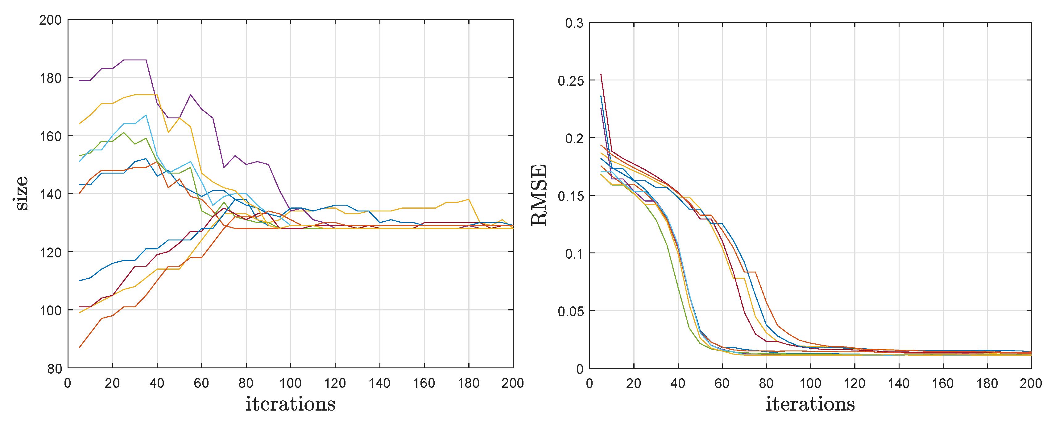
Finally, we partially justify our choices for the number of iterations. Generally, the rule is simple: more iterations lead to better results. However, there are many factors that influence the convergence speed and there are many random elements in the algorithm (the initial dictionary, the added atoms, the initial size and, of course, the noise). We illustrate in Figure 1 the evolution of the main variables, the current dictionary size (as given by the ITC) and RMSE (on the training data), for , and 10 runs of ITC-ADL with random initial sizes. The values are shown for iterations that are multiple of c; the size is constant between them and the RMSE typically decreases. It is visible that, after 100 iterations, the size is close to the true one and the RMSE is at about its final (and almost optimal, as we have seen) value. Typically, the size becomes larger than the true one when the RMSE reaches the lowest value. Then, ITC-ADL gradually trims the dictionary almost without changing the RMSE. Thus, if our purpose is dictionary learning (and perfect recovery is not sought because there is actually no true dictionary), the number of iterations can be smaller than for dictionary recovery.
4.3. Experiments with Unknown Sparsity Level
Using the same setup as in Section 4.1, we run ITC-ADL with several values of s, not only the true one, and choose the sparsity level that gives the best ITC value. Otherwise, the algorithm is unchanged and estimates the dictionary size as usual. Table 9 presents the average values of the sparsity level and of the dictionary size given by the above procedure for .
The variance of the estimated s is very low: typically, only two values are obtained. For example, when , for SNR = 10 dB, only values of 6 and 7 are obtained; when SNR=40 dB, only values of 8 and 9 are obtained; etc. One can see that the sparsity level estimations are rather accurate; the only deviation is at low SNR, when s is underestimated. The dictionary size is well estimated, in accordance with the previous results.
A competing algorithm is Adaptive ITKrM [9] (Matlab sources available at https://www.uibk.ac.at/mathematik/personal/schnass/code/adl.zip), reported to give very good results in DR problems. However, it seems that this algorithm needs more signals than ours. In our setup with , A-ITKrM gives very poor results. Table 10 gives results for N = 20,000, where A-ITKrM becomes competitive. Due to time constraints, the results are averaged over only 20 runs. The table shows the obtained average sparsity level, dictionary size, and ratio RMSE/RMSEi, where RMSE is the error of our algorithm (using ERNML) and RMSEi is the error of A-ITKrM. Since A-ITKrM severely underestimates s, we have computed RMSEi (and RMSE) using OMP with the true s. Even so, our algorithm finds a more accurate version of the dictionary. While ITKrM gives very good estimates of n and a good approximation of the dictionary, it seems unable to refine the dictionary as well as our algorithm.
In the current unoptimized implementations, the execution times of ITC-ADL and A-ITKrM are comparable, our algorithm being faster for small s and slower for large s. Limited trials with N = 50,000 suggest that the above remarks continue to stand true.
5. Conclusions
We present a dictionary learning algorithm that works for unknown dictionary size. Using specialized Information Theoretic Criteria, based on BIC and RNML, the size is adapted during the evolution of a standard DL algorithm (AK-SVD in our case). Experimental results show that the algorithm is able to discover the true size of the dictionary used to generate data and, somewhat surprisingly, can give better results than AK-SVD run with the true size.
There are several possible directions for future research. Testing ITC-ADL in various applications is a first aim; they can range from direct applications, such as denoising or missing data estimation (inpainting), to more complex ones, e.g. classification. We also plan to combine the ITC idea with other DL algorithms, not only AK-SVD, especially with algorithms for which the sparsity level is not the same for all signals. Another direction is to find ITC that are suited for other types of noise, not Gaussian as here, with the final purpose of obtaining a single tool that analyzes data, finds the appropriate sparse representation model and designs the optimal dictionary.
Author Contributions
Conceptualization, B.D.; methodology, B.D. and C.D.G.; software, B.D. and C.D.G.; validation, B.D. and C.D.G.; formal analysis, B.D. and C.D.G.; investigation, B.D. and C.D.G.; writing—original draft preparation, B.D.; writing—review and editing, B.D. and C.D.G.; and visualization, B.D. and C.D.G.
Funding
This research received no external funding.
Conflicts of Interest
The authors declare no conflict of interest.
Appendix A
We present here more numerical results for supporting our algorithm. The setup is that already described in Section 4.
1. Known sparsity level. For each dictionary size , we present three tables with results obtained with the two criteria, ERNML and EBIC. (Some of the tables have already been presented in the main body of this paper and are only mentioned again here for full reference.) The first gives the average, minimum and maximum size n computed by ITC-ADL. The second shows RMSE information on the training data and the third shows RMSE information on test data. These tables are as follows: for , Table 1, Table A1 and Table 2; for , Table A2, Table A3 and Table A4 (the size takes random values between 120 and 280); and for , Table 3, Table A5 and Table 4.
2. Unknown sparsity level. Results for are given in Table A6.

Table A1.
Ratios RMSE/RMSE and RMSE/RMSE on the training data, when . Left: ERNML. Right: EBIC.
| SNR (dB) | 6 | 8 | 10 | 12 | SNR (dB) | 6 | 8 | 10 | 12 | ||
|---|---|---|---|---|---|---|---|---|---|---|---|
| 10 | 0.9798 | 0.9772 | 0.9742 | 0.9701 | 0.9709 | 10 | 0.9800 | 0.9775 | 0.9744 | 0.9726 | 0.9873 |
| 0.9536 | 0.9758 | 0.9815 | 0.9882 | 0.9844 | 0.9539 | 0.9760 | 0.9817 | 0.9908 | 1.0011 | ||
| 20 | 0.9820 | 0.9815 | 0.9820 | 0.9812 | 0.9837 | 20 | 0.9831 | 0.9810 | 0.9815 | 0.9848 | 0.9941 |
| 0.7512 | 0.8515 | 0.8874 | 0.9205 | 0.9306 | 0.7520 | 0.8511 | 0.8870 | 0.9238 | 0.9404 | ||
| 30 | 0.9828 | 0.9954 | 1.0035 | 1.0213 | 1.0733 | 30 | 1.0015 | 0.9870 | 1.0061 | 1.0399 | 1.1056 |
| 0.3473 | 0.4944 | 0.6410 | 0.7268 | 0.7691 | 0.3543 | 0.4915 | 0.6453 | 0.7375 | 0.7905 | ||
| 40 | 0.9829 | 0.9844 | 1.1721 | 1.2104 | 1.2899 | 40 | 0.9837 | 1.0131 | 1.1004 | 1.2865 | 1.4669 |
| 0.1556 | 0.2464 | 0.5640 | 0.5444 | 0.5843 | 0.1557 | 0.2505 | 0.5309 | 0.5972 | 0.6738 |
Table A2.
Minimum (top), average (middle) and maximum (bottom) sizes computed when . Left: ERNML. Right: EBIC.
Table A2.
Minimum (top), average (middle) and maximum (bottom) sizes computed when . Left: ERNML. Right: EBIC.
| SNR (dB) | 6 | 8 | 10 | 12 | SNR (dB) | 6 | 8 | 10 | 12 | ||
|---|---|---|---|---|---|---|---|---|---|---|---|
| 192 | 192 | 192 | 191 | 193 | 192 | 192 | 192 | 185 | 170 | ||
| 10 | 193.20 | 192.52 | 192.10 | 192.44 | 284.18 | 10 | 193.30 | 192.40 | 192.02 | 191.60 | 190.52 |
| 203 | 199 | 195 | 198 | 471 | 203 | 201 | 193 | 193 | 200 | ||
| 192 | 192 | 192 | 192 | 192 | 192 | 192 | 192 | 192 | 192 | ||
| 20 | 193.02 | 192.38 | 192.16 | 192.14 | 192.10 | 20 | 193.40 | 192.40 | 192.20 | 192.10 | 192.28 |
| 199 | 195 | 194 | 194 | 194 | 217 | 195 | 195 | 194 | 195 | ||
| 192 | 192 | 192 | 192 | 192 | 192 | 192 | 192 | 192 | 192 | ||
| 30 | 192.80 | 192.38 | 193.56 | 194.40 | 195.94 | 30 | 192.70 | 192.38 | 192.86 | 194.38 | 195.06 |
| 204 | 194 | 202 | 219 | 219 | 200 | 194 | 197 | 202 | 211 | ||
| 192 | 192 | 192 | 192 | 192 | 192 | 192 | 192 | 192 | 192 | ||
| 40 | 195.68 | 193.92 | 194.18 | 199.70 | 200.78 | 40 | 194.34 | 193.92 | 193.98 | 197.06 | 199.38 |
| 268 | 260 | 217 | 271 | 329 | 269 | 260 | 208 | 222 | 230 |
Table A3.
Ratios RMSE/RMSE and RMSE/RMSE on the training data, when . Left ERNML. Right: EBIC.
| SNR (dB) | 6 | 8 | 10 | 12 | SNR (dB) | 6 | 8 | 10 | 12 | ||
|---|---|---|---|---|---|---|---|---|---|---|---|
| 10 | 0.9702 | 0.9659 | 0.9604 | 0.9538 | 0.9388 | 10 | 0.9702 | 0.9661 | 0.9611 | 0.9636 | 1.0214 |
| 0.9541 | 0.9739 | 0.9803 | 0.9818 | 0.9560 | 0.9542 | 0.9741 | 0.9809 | 0.9920 | 1.0401 | ||
| 20 | 0.9764 | 0.9715 | 0.9702 | 0.9694 | 0.9684 | 20 | 0.9750 | 0.9711 | 0.9697 | 0.9704 | 0.9805 |
| 0.7464 | 0.8375 | 0.8649 | 0.8916 | 0.8764 | 0.7452 | 0.8371 | 0.8645 | 0.8925 | 0.8872 | ||
| 30 | 0.9773 | 0.9826 | 0.9782 | 0.9869 | 0.9768 | 30 | 0.9758 | 0.9727 | 0.9841 | 1.0060 | 1.0483 |
| 0.3388 | 0.4551 | 0.5476 | 0.6219 | 0.6722 | 0.3383 | 0.4507 | 0.5516 | 0.6326 | 0.7190 | ||
| 40 | 1.1138 | 1.0270 | 1.0029 | 1.0568 | 1.0202 | 40 | 1.0361 | 0.9898 | 1.0243 | 1.1392 | 1.1162 |
| 0.1525 | 0.1830 | 0.3688 | 0.5038 | 0.4862 | 0.1447 | 0.1765 | 0.3751 | 0.5360 | 0.5331 |
Table A4.
Ratios RMSE/RMSE and RMSE/RMSE on test data, when . Left: ERNML. Right: EBIC.
| SNR (dB) | 6 | 8 | 10 | 12 | SNR (dB) | 6 | 8 | 10 | 12 | ||
|---|---|---|---|---|---|---|---|---|---|---|---|
| 10 | 1.0307 | 1.0359 | 1.0426 | 1.0531 | 1.0994 | 10 | 1.0306 | 1.0358 | 1.0429 | 1.0633 | 1.1467 |
| 0.9441 | 0.9703 | 0.9780 | 0.9794 | 0.9944 | 0.9440 | 0.9703 | 0.9783 | 0.9890 | 1.0371 | ||
| 20 | 1.0323 | 1.0302 | 1.0344 | 1.0396 | 1.0470 | 20 | 1.0311 | 1.0297 | 1.0339 | 1.0396 | 1.0579 |
| 0.7156 | 0.8179 | 0.8519 | 0.8825 | 0.8644 | 0.7148 | 0.8175 | 0.8514 | 0.8825 | 0.8733 | ||
| 30 | 1.0307 | 1.0403 | 1.0497 | 1.0624 | 1.0679 | 30 | 1.0306 | 1.0289 | 1.0492 | 1.0781 | 1.1302 |
| 0.3152 | 0.4260 | 0.5355 | 0.6045 | 0.6787 | 0.3152 | 0.4214 | 0.5355 | 0.6113 | 0.7179 | ||
| 40 | 1.1950 | 1.1187 | 1.0985 | 1.2153 | 1.1240 | 40 | 1.1135 | 1.0603 | 1.0940 | 1.2805 | 1.2214 |
| 0.1488 | 0.1761 | 0.3760 | 0.5180 | 0.4814 | 0.1383 | 0.1678 | 0.3725 | 0.5369 | 0.5312 |
Table A5.
Ratios RMSE/RMSE and RMSE/RMSE on the training data, when . Left: ERNML. Right: EBIC.
| SNR (dB) | 6 | 8 | 10 | 12 | SNR (dB) | 6 | 8 | 10 | 12 | ||
|---|---|---|---|---|---|---|---|---|---|---|---|
| 10 | 0.9600 | 0.9543 | 0.9464 | 0.8946 | 1.0978 | 10 | 0.9599 | 0.9548 | 0.9717 | 1.0241 | 1.2422 |
| 0.9543 | 0.9731 | 0.9751 | 0.9363 | 0.8748 | 0.9542 | 0.9736 | 1.0012 | 1.0716 | 0.9896 | ||
| 20 | 0.9644 | 0.9617 | 0.9583 | 0.9555 | 0.9560 | 20 | 0.9635 | 0.9620 | 0.9601 | 0.9612 | 1.0299 |
| 0.7466 | 0.8394 | 0.8505 | 0.8623 | 0.8897 | 0.7459 | 0.8397 | 0.8521 | 0.8674 | 0.9616 | ||
| 30 | 0.9813 | 0.9645 | 0.9615 | 0.9544 | 1.0171 | 30 | 0.9786 | 0.9669 | 0.9719 | 0.9830 | 1.1147 |
| 0.3420 | 0.4440 | 0.5221 | 0.5669 | 0.6956 | 0.3416 | 0.4448 | 0.5287 | 0.5821 | 0.7571 | ||
| 40 | 1.0104 | 0.9607 | 0.9248 | 0.9386 | 1.0586 | 40 | 1.0327 | 0.9502 | 0.9468 | 1.0250 | 1.1443 |
| 0.1253 | 0.1821 | 0.2379 | 0.3860 | 0.5270 | 0.1278 | 0.1802 | 0.2421 | 0.4177 | 0.5719 |
Table A6.
Average values of s (top) and n (bottom), when . Left: ERNML. Right: EBIC.
| SNR (dB) | 6 | 8 | 10 | 12 | SNR (dB) | 6 | 8 | 10 | 12 | ||
|---|---|---|---|---|---|---|---|---|---|---|---|
| 10 | 4.00 | 5.00 | 6.24 | 7.28 | 8.04 | 10 | 3.98 | 4.20 | 4.96 | 6.00 | 8.00 |
| 194.26 | 193.22 | 192.18 | 192.26 | 200.42 | 193.66 | 192.54 | 192.60 | 189.00 | 179.04 | ||
| 20 | 4.00 | 6.00 | 8.02 | 9.98 | 11.34 | 20 | 4.00 | 6.00 | 8.00 | 9.52 | 10.84 |
| 193.44 | 192.40 | 192.46 | 192.22 | 194.66 | 193.84 | 192.22 | 192.18 | 192.10 | 192.32 | ||
| 30 | 4.10 | 6.00 | 8.12 | 10.20 | 12.24 | 30 | 4.00 | 6.06 | 8.08 | 10.10 | 12.00 |
| 193.12 | 192.48 | 193.30 | 196.24 | 199.38 | 193.16 | 192.68 | 192.84 | 194.74 | 195.02 | ||
| 40 | 4.00 | 6.04 | 8.18 | 10.58 | 12.28 | 40 | 4.06 | 6.06 | 8.22 | 10.68 | 12.16 |
| 192.64 | 192.72 | 195.58 | 201.98 | 208.30 | 193.86 | 193.04 | 194.40 | 202.26 | 201.56 |
References
- Rubinstein, R.; Bruckstein, A.; Elad, M. Dictionaries for Sparse Representations Modeling. Proc. IEEE 2010, 98, 1045–1057. [Google Scholar] [CrossRef]
- Tosic, I.; Frossard, P. Dictionary Learning. IEEE Signal Proc. Mag. 2011, 28, 27–38. [Google Scholar] [CrossRef]
- Dumitrescu, B.; Irofti, P. Dictionary Learning Algorithms and Applications; Springer: Berlin, Germany, 2018. [Google Scholar]
- Agarwal, A.; Anandkumar, A.; Jain, P.; Netrapalli, P.; Tandon, R. Learning sparsely used overcomplete dictionaries. In Proceedings of the Conference on Learning Theory, Barcelona, Spain, 13–15 June 2014; pp. 123–137. [Google Scholar]
- Arora, S.; Ge, R.; Moitra, A. New algorithms for learning incoherent and overcomplete dictionaries. In Proceedings of the Conference on Learning Theory, Barcelona, Spain, 13–15 June 2014; pp. 779–806. [Google Scholar]
- Hillar, C.; Sommer, F. When can dictionary learning uniquely recover sparse data from subsamples? IEEE Trans. Inf. Theory 2015, 61, 6290–6297. [Google Scholar] [CrossRef]
- Sun, J.; Qu, Q.; Wright, J. Complete dictionary recovery over the sphere I: Overview and the geometric picture. IEEE Trans. Inf. Theory 2017, 63, 853–884. [Google Scholar] [CrossRef]
- Ramirez, I.; Sapiro, G. An MDL framework for sparse coding and dictionary learning. IEEE Trans. Signal Proc. 2012, 60, 2913–2927. [Google Scholar] [CrossRef]
- Schnass, K. Dictionary learning-from local towards global and adaptive. arXiv 2018, arXiv:1804.07101. [Google Scholar]
- Rusu, C.; Dumitrescu, B. Stagewise K-SVD to Design Efficient Dictionaries for Sparse Representations. IEEE Signal Proc. Lett. 2012, 19, 631–634. [Google Scholar] [CrossRef]
- Marsousi, M.; Abhari, K.; Babyn, P.; Alirezaie, J. An Adaptive Approach to Learn Overcomplete Dictionaries With Efficient Numbers of Elements. IEEE Trans. Signal Proc. 2014, 62, 3272–3283. [Google Scholar] [CrossRef]
- Feng, J.; Song, L.; Yang, X.; Zhang, W. Sub clustering K-SVD: Size variable dictionary learning for sparse representations. In Proceedings of the 2009 16th IEEE International Conference on Image Processing (ICIP), Cairo, Egypt, 7–10 November 2009; pp. 2149–2152. [Google Scholar]
- Mazhar, R.; Gader, P.D. EK-SVD: Optimized Dictionary Design for Sparse Representations. In Proceedings of the 2008 19th International Conference on Pattern Recognition, Tampa, FL, USA, 8–11 December 2008; pp. 1–4. [Google Scholar]
- Rao, N.; Porikli, F. A Clustering Approach to Optimize Online Dictionary Learning. In Proceedings of the International Conference on Acoustics Speech Signal Proc. (ICASSP), Kyoto, Japan, 25–30 March 2012; pp. 1293–1296. [Google Scholar]
- Yaghoobi, M.; Blumensath, T.; Davies, M. Dictionary Learning for Sparse Approximations with the Majorization Method. IEEE Trans. Signal Proc. 2009, 57, 2178–2191. [Google Scholar] [CrossRef]
- Dang, H.; Chainais, P. Towards dictionaries of optimal size: a Bayesian non parametric approach. J. Signal Proc. Syst. 2018, 90, 221–232. [Google Scholar] [CrossRef]
- Zhou, M.; Chen, H.; Paisley, J.; Ren, L.; Li, L.; Xing, Z.; Dunson, D.; Sapiro, G.; Carin, L. Nonparametric Bayesian Dictionary Learning for Analysis of Noisy and Incomplete Images. IEEE Trans. Image Proc. 2012, 21, 130–144. [Google Scholar] [CrossRef] [PubMed]
- Huang, Y.; Paisley, J.; Lin, Q.; Ding, X.; Fu, X.; Zhang, X. Bayesian nonparametric dictionary learning for compressed sensing MRI. IEEE Trans. Image Proc. 2014, 23, 5007–5019. [Google Scholar] [CrossRef] [PubMed]
- Jung, A.; Eldar, Y.; Görtz, N. On the minimax risk of dictionary learning. IEEE Trans. Inf. Theory 2016, 62, 1501–1515. [Google Scholar] [CrossRef]
- Schwarz, G. Estimating the Dimension of a Model. Ann. Stat. 1978, 6, 461–464. [Google Scholar] [CrossRef]
- Chen, J.; Chen, Z. Extended Bayesian information criteria for model selection with large model spaces. Biometrika 2008, 95, 759–771. [Google Scholar] [CrossRef] [Green Version]
- Rissanen, J. MDL denoising. IEEE Trans. Inf. Theory 2000, 46, 2537–2543. [Google Scholar] [CrossRef]
- Rissanen, J. Information and Complexity in Statistical Modeling; Springer: Heidelberg, Germany, 2007. [Google Scholar]
- Roos, T.; Myllymäki, P.; Rissanen, J. MDL denoising revisited. IEEE Trans. Signal Proc. 2009, 57, 3347–3360. [Google Scholar] [CrossRef]
- Liski, E.; Liski, A. Minimum Description Length Model Selection in Gaussian Regression under Data Constraints. In Statistical Inference, Econometric Analysis and Matrix Algebra; Schipp, B., Kräer, W., Eds.; Physica-Verlag: Heidelberg, Germany, 2009; pp. 201–208. [Google Scholar]
- Giurcăneanu, C.; Razavi, S.; Liski, A. Variable selection in linear regression: Several approaches based on normalized maximum likelihood. Signal Process. 2011, 91, 1671–1692. [Google Scholar] [CrossRef] [Green Version]
- Akaike, H. Autoregressive model fitting for control. Ann. Inst. Stat. Math. 1971, 23, 163–180. [Google Scholar] [CrossRef]
- Hannan, E.J.; Quinn, B.G. The Determination of the Order of an Autoregression. J. R. Stat. Soc. Ser. B (Methodol.) 1979, 41, 190–195. [Google Scholar] [CrossRef]
- Pati, Y.; Rezaiifar, R.; Krishnaprasad, P. Orthogonal Matching Pursuit: Recursive Function Approximation with Applications to Wavelet Decomposition. In Proceedings of the 27th Asilomar Conference on Signals, Systems and Computers, Pacific Grove, CA, USA, 1–3 November 1993; Volume 1, pp. 40–44. [Google Scholar]
- Rubinstein, R.; Zibulevsky, M.; Elad, M. Efficient Implementation of the K-SVD Algorithm Using Batch Orthogonal Matching Pursuit; Technical Report CS-2008-08; Technion University: Haifa, Israel, 2008. [Google Scholar]
Figure 1.
Evolution of the dictionary size (left) and of the RMSE (right) during 10 runs of ITC-ADL, with , .
Figure 1.
Evolution of the dictionary size (left) and of the RMSE (right) during 10 runs of ITC-ADL, with , .

Table 1.
Minimum (top), average (middle) and maximum (bottom) sizes computed when . Left: ERNML. Right: EBIC.
Table 1.
Minimum (top), average (middle) and maximum (bottom) sizes computed when . Left: ERNML. Right: EBIC.
| SNR (dB) | 6 | 8 | 10 | 12 | SNR (dB) | 6 | 8 | 10 | 12 | ||
|---|---|---|---|---|---|---|---|---|---|---|---|
| 128 | 128 | 128 | 128 | 128 | 128 | 128 | 128 | 128 | 124 | ||
| 10 | 129.02 | 128.22 | 128.04 | 128.12 | 129.74 | 10 | 128.82 | 128.24 | 128.00 | 128.06 | 127.86 |
| 143 | 132 | 130 | 130 | 143 | 143 | 135 | 128 | 129 | 130 | ||
| 128 | 128 | 128 | 128 | 128 | 128 | 128 | 128 | 128 | 128 | ||
| 20 | 128.20 | 128.06 | 128.06 | 128.18 | 128.34 | 20 | 128.22 | 128.14 | 128.12 | 128.06 | 128.30 |
| 130 | 129 | 129 | 131 | 137 | 130 | 131 | 132 | 129 | 131 | ||
| 128 | 128 | 128 | 128 | 128 | 128 | 128 | 128 | 128 | 128 | ||
| 30 | 128.18 | 128.14 | 128.26 | 128.24 | 128.94 | 30 | 128.18 | 128.10 | 128.24 | 128.76 | 129.18 |
| 129 | 133 | 130 | 131 | 138 | 130 | 129 | 132 | 133 | 135 | ||
| 128 | 128 | 128 | 128 | 128 | 128 | 128 | 128 | 128 | 128 | ||
| 40 | 128.18 | 128.08 | 128.70 | 128.78 | 130.00 | 40 | 128.12 | 128.36 | 128.88 | 129.04 | 129.08 |
| 129 | 129 | 143 | 132 | 140 | 129 | 132 | 133 | 137 | 132 |
Table 2.
Ratios RMSE/RMSE and RMSE/RMSE on test data, when . Left: ERNML. Right: EBIC.
| SNR (dB) | 6 | 8 | 10 | 12 | SNR (dB) | 6 | 8 | 10 | 12 | ||
|---|---|---|---|---|---|---|---|---|---|---|---|
| 10 | 1.0194 | 1.0224 | 1.0258 | 1.0313 | 1.0402 | 10 | 1.0194 | 1.0224 | 1.0257 | 1.0327 | 1.0553 |
| 0.9482 | 0.9741 | 0.9809 | 0.9883 | 0.9820 | 0.9482 | 0.9741 | 0.9808 | 0.9896 | 0.9964 | ||
| 20 | 1.0181 | 1.0203 | 1.0235 | 1.0256 | 1.0319 | 20 | 1.0190 | 1.0192 | 1.0227 | 1.0296 | 1.0417 |
| 0.7326 | 0.8360 | 0.8792 | 0.9153 | 0.9231 | 0.7332 | 0.8352 | 0.8786 | 0.9187 | 0.9318 | ||
| 30 | 1.0178 | 1.0310 | 1.0432 | 1.0572 | 1.1006 | 30 | 1.0380 | 1.0228 | 1.0445 | 1.0776 | 1.1427 |
| 0.3257 | 0.4835 | 0.6283 | 0.7133 | 0.7467 | 0.3323 | 0.4809 | 0.6310 | 0.7242 | 0.7722 | ||
| 40 | 1.0177 | 1.0181 | 1.2080 | 1.1955 | 1.3554 | 40 | 1.0177 | 1.0536 | 1.1560 | 1.3266 | 1.5319 |
| 0.1516 | 0.2402 | 0.5606 | 0.5114 | 0.5721 | 0.1516 | 0.2459 | 0.5399 | 0.5857 | 0.6495 |
Table 3.
Minimum (top), average (middle) and maximum (bottom) sizes computed when . Left: ERNML. Right: EBIC.
Table 3.
Minimum (top), average (middle) and maximum (bottom) sizes computed when . Left: ERNML. Right: EBIC.
| SNR (dB) | 6 | 8 | 10 | 12 | SNR (dB) | 6 | 8 | 10 | 12 | ||
|---|---|---|---|---|---|---|---|---|---|---|---|
| 256 | 256 | 256 | 254 | 330 | 256 | 256 | 222 | 206 | 225 | ||
| 10 | 258.74 | 256.88 | 256.64 | 346.60 | 444.28 | 10 | 258.46 | 256.32 | 253.40 | 246.30 | 308.10 |
| 268 | 270 | 261 | 566 | 616 | 277 | 260 | 257 | 257 | 386 | ||
| 255 | 256 | 256 | 256 | 256 | 256 | 256 | 256 | 256 | 239 | ||
| 20 | 259.80 | 256.54 | 256.50 | 256.62 | 267.36 | 20 | 259.30 | 256.84 | 256.36 | 256.42 | 256.04 |
| 288 | 261 | 260 | 260 | 444 | 275 | 261 | 260 | 260 | 273 | ||
| 256 | 256 | 256 | 256 | 256 | 256 | 256 | 256 | 256 | 236 | ||
| 30 | 258.90 | 261.98 | 260.32 | 269.66 | 325.76 | 30 | 258.84 | 261.02 | 258.12 | 261.86 | 263.68 |
| 312 | 335 | 357 | 374 | 477 | 312 | 329 | 267 | 287 | 291 | ||
| 256 | 256 | 256 | 256 | 256 | 256 | 256 | 256 | 256 | 256 | ||
| 40 | 267.02 | 261.50 | 271.12 | 304.62 | 324.72 | 40 | 265.12 | 260.12 | 260.80 | 275.56 | 268.28 |
| 343 | 343 | 357 | 422 | 489 | 343 | 336 | 283 | 320 | 322 |
Table 4.
Ratios RMSE/RMSE and RMSE/RMSE on test data, when . Left: ERNML. Right: EBIC.
| SNR (dB) | 6 | 8 | 10 | 12 | SNR (dB) | 6 | 8 | 10 | 12 | ||
|---|---|---|---|---|---|---|---|---|---|---|---|
| 10 | 1.0427 | 1.0500 | 1.0617 | 1.0859 | 1.4794 | 10 | 1.0426 | 1.0504 | 1.0905 | 1.1843 | 1.5705 |
| 0.9430 | 0.9670 | 0.9717 | 0.9835 | 0.9540 | 0.9429 | 0.9674 | 0.9981 | 1.0723 | 1.0123 | ||
| 20 | 1.0400 | 1.0408 | 1.0448 | 1.0508 | 1.0646 | 20 | 1.0385 | 1.0414 | 1.0466 | 1.0563 | 1.1320 |
| 0.7105 | 0.8184 | 0.8342 | 0.8434 | 0.8792 | 0.7095 | 0.8189 | 0.8356 | 0.8479 | 0.9375 | ||
| 30 | 1.0568 | 1.0482 | 1.0488 | 1.0616 | 1.1677 | 30 | 1.0535 | 1.0466 | 1.0610 | 1.0882 | 1.2282 |
| 0.3024 | 0.4160 | 0.4996 | 0.5599 | 0.7156 | 0.3017 | 0.4152 | 0.5066 | 0.5718 | 0.7482 | ||
| 40 | 1.1130 | 1.0600 | 1.1090 | 1.2461 | 1.3096 | 40 | 1.1304 | 1.0574 | 1.0790 | 1.2541 | 1.2866 |
| 0.1147 | 0.1647 | 0.2471 | 0.4346 | 0.5666 | 0.1164 | 0.1627 | 0.2410 | 0.4363 | 0.5613 |
Table 5.
Average execution times (in seconds) of ITC-ADL (with ERNML) and AK-SVD.
| n | Algorithm | 6 | 8 | 10 | 12 | |
|---|---|---|---|---|---|---|
| 128 | ITC-ADL | 39.2 | 52.1 | 66.6 | 83.7 | 104.6 |
| AK-SVD | 10.3 | 14.2 | 17.9 | 22.0 | 26.4 | |
| 192 | ITC-ADL | 75.0 | 101.8 | 133.2 | 165.9 | 212.6 |
| AK-SVD | 20.3 | 28.5 | 36.3 | 44.2 | 52.6 | |
| 256 | ITC-ADL | 121.9 | 162.2 | 212.1 | 267.0 | 374.2 |
| AK-SVD | 36.0 | 48.5 | 63.0 | 75.9 | 90.7 |
Table 6.
Average dictionary sizes given by ITC-ADL, for , , when vary.
| 2 | 3 | 4 | 5 | 6 | 7 | 8 | |
|---|---|---|---|---|---|---|---|
| size | 257.90 | 257.88 | 257.88 | 258.16 | 259.86 | 258.16 | 259.24 |
Table 7.
Average dictionary sizes given by ITC-ADL, for , for several values of .
| 15 | 20 | 25 | ||
|---|---|---|---|---|
| 263.86 | 258.34 | 257.30 | 256.80 | |
| 288.18 | 286.68 | 280.66 | 274.84 |
Table 8.
Average dictionary sizes given by ITC-ADL, for , for several values of c.
| 4 | 5 | 6 | 8 | 10 | ||
|---|---|---|---|---|---|---|
| 257.16 | 258.04 | 258.32 | 256.92 | 257.28 | 256.96 | |
| 265.36 | 273.00 | 280.36 | 285.46 | 282.64 | 284.02 |
Table 9.
Average values of s (top) and n (bottom), when . Left: ERNML. Right: EBIC.
| SNR (dB) | 6 | 8 | 10 | 12 | SNR (dB) | 6 | 8 | 10 | 12 | ||
|---|---|---|---|---|---|---|---|---|---|---|---|
| 10 | 4.00 | 5.10 | 6.90 | 7.88 | 8.24 | 10 | 3.98 | 4.64 | 5.00 | 6.00 | 8.00 |
| 128.38 | 128.14 | 128.04 | 128.02 | 128.04 | 128.78 | 128.10 | 128.10 | 128.12 | 127.88 | ||
| 20 | 4.00 | 6.00 | 8.00 | 10.00 | 11.86 | 20 | 4.00 | 6.00 | 8.00 | 9.76 | 11.10 |
| 128.14 | 128.02 | 128.12 | 128.16 | 128.00 | 128.28 | 128.02 | 128.10 | 128.14 | 128.16 | ||
| 30 | 4.02 | 6.00 | 8.06 | 10.18 | 12.16 | 30 | 4.04 | 6.00 | 8.08 | 10.12 | 12.30 |
| 128.04 | 128.14 | 128.52 | 128.46 | 129.16 | 128.14 | 128.04 | 128.56 | 128.78 | 129.56 | ||
| 40 | 4.04 | 6.10 | 8.16 | 10.42 | 12.40 | 40 | 4.00 | 6.04 | 8.14 | 10.48 | 12.60 |
| 128.22 | 128.72 | 129.36 | 132.66 | 132.52 | 128.12 | 128.66 | 130.18 | 130.34 | 132.76 |
Table 10.
Results with A-ITKrM: average values of s (top), n (middle) and RMSE/RMSE (bottom).
| SNR (dB) | 6 | 8 | 10 | 12 | |
|---|---|---|---|---|---|
| 3.00 | 3.00 | 3.00 | 3.00 | 3.00 | |
| 10 | 128.00 | 127.85 | 126.40 | 123.55 | 123.20 |
| 0.9906 | 0.9856 | 0.9545 | 0.9045 | 0.8995 | |
| 3.00 | 4.00 | 4.00 | 4.00 | 4.00 | |
| 20 | 128.00 | 128.00 | 128.00 | 128.00 | 128.50 |
| 0.9454 | 0.9113 | 0.8821 | 0.8544 | 0.8217 | |
| 3.00 | 4.00 | 4.00 | 4.00 | 4.00 | |
| 30 | 128.00 | 128.00 | 128.00 | 128.00 | 128.55 |
| 0.6906 | 0.5830 | 0.5186 | 0.4830 | 0.4564 | |
| 3.00 | 4.00 | 4.00 | 4.00 | 4.00 | |
| 40 | 128.00 | 128.00 | 128.00 | 128.05 | 128.45 |
| 0.2868 | 0.2247 | 0.2234 | 0.2462 | 0.3249 |
© 2019 by the authors. Licensee MDPI, Basel, Switzerland. This article is an open access article distributed under the terms and conditions of the Creative Commons Attribution (CC BY) license (http://creativecommons.org/licenses/by/4.0/).
Share and Cite
MDPI and ACS Style
Dumitrescu, B.; Giurcăneanu, C.D. Adaptive-Size Dictionary Learning Using Information Theoretic Criteria. Algorithms 2019, 12, 178. https://0-doi-org.brum.beds.ac.uk/10.3390/a12090178
AMA Style
Dumitrescu B, Giurcăneanu CD. Adaptive-Size Dictionary Learning Using Information Theoretic Criteria. Algorithms. 2019; 12(9):178. https://0-doi-org.brum.beds.ac.uk/10.3390/a12090178
Chicago/Turabian StyleDumitrescu, Bogdan, and Ciprian Doru Giurcăneanu. 2019. "Adaptive-Size Dictionary Learning Using Information Theoretic Criteria" Algorithms 12, no. 9: 178. https://0-doi-org.brum.beds.ac.uk/10.3390/a12090178
Note that from the first issue of 2016, this journal uses article numbers instead of page numbers. See further details here.