Feedback-Based Integration of the Whole Process of Data Anonymization in a Graphical Interface


1
Methods Unit, Statistics Austria, 1110 Vienna, Austria
2
Institute for Data Analysis and Process Design, Zurich University of Applied Sciences, 8400 Winterthur, Switzerland
*
Author to whom correspondence should be addressed.
Algorithms 2019, 12(9), 191; https://0-doi-org.brum.beds.ac.uk/10.3390/a12090191
Submission received: 23 July 2019
/
Revised: 5 September 2019
/
Accepted: 5 September 2019
/
Published: 10 September 2019
(This article belongs to the Special Issue Statistical Disclosure Control for Microdata)
Abstract
:The interactive, web-based point-and-click application presented in this article, allows anonymizing data without any knowledge in a programming language. Anonymization in data mining, but creating safe, anonymized data is by no means a trivial task. Both the methodological issues as well as know-how from subject matter specialists should be taken into account when anonymizing data. Even though specialized software such as sdcMicro exists, it is often difficult for nonexperts in a particular software and without programming skills to actually anonymize datasets without an appropriate app. The presented app is not restricted to apply disclosure limitation techniques but rather facilitates the entire anonymization process. This interface allows uploading data to the system, modifying them and to create an object defining the disclosure scenario. Once such a statistical disclosure control (SDC) problem has been defined, users can apply anonymization techniques to this object and get instant feedback on the impact on risk and data utility after SDC methods have been applied. Additional features, such as an Undo Button, the possibility to export the anonymized dataset or the required code for reproducibility reasons, as well its interactive features, make it convenient both for experts and nonexperts in R—the free software environment for statistical computing and graphics—to protect a dataset using this app.
1. Introduction
Various anonymization software tools have been made available in the past. One of the most feature-rich is sdcMicro [1,2], an R package for data anonymization optimized for large datasets. For users comfortable with using R, this package provides a tool for the application of a comprehensive suite of methods commonly used and described in literature on disclosure control. However, the application of these methods proved to be difficult for nonexperts in R to create secure and anonymous datasets.
GUIssupport nonexperts in programming to anonymize their datasets. Ideally, a graphical user interface in this area not only allows to access and apply methods, but it additionally helps to integrate the entire workflow and anonymization process on data anonymization and offers additional tools and user guidance. Several graphical user interfaces in this area have been developed in the past and for comparison reasons, we want to outline the most prominent ones.
1.1. Outline and Brief Comparison of Graphical User Interfaces for SDC
One of the first graphical user interfaces was provided via the software -Argus [3]. The software is still developed and maintained by Statistics Netherlands and other partners, and some of those extensions are being subsidized by Eurostat. The software features a graphical point and click user interface, which was based on “Visual Basic” until version 4.2., and is now (Version 5.1. and onwards) written using “Java” and can be downloaded for free from the CASC website (http://neon.vb.cbs.nl/casc/mu.htm). Currently, only 32-bit versions have been built, and there is no command line interface available. The tool uses a certain range of different statistical anonymization methods such as global re-coding (grouping of categories), local suppression, randomization, adding noise, microaggregation and top- and bottom-coding.
A number of tools with a graphical user interface are available for basic frequency calculation and for ensuring k-anonymity, l-diversity, and similar frequency calculations. TIAMAT [4] is a visual tool allowing data publishers to select a suitable k-anonymization transformation and its corresponding parameters in order to protect their data. Since it does not support additional methods, it is not considered in the following. This is also true for PARAT (version 6) that is based on frequency calculations only. OpenAnonymizer is based on the concepts of k-anonymity and l-diversity only, and thus will not considered further. Also, SECRETA [5] is not considered because of its limited features; for example, there is no internal risk estimation available in this tool.
Amnesia [6] (version 1.0.6) is a data anonymization tool developed at the Athena Research Center. Amnesia has an hierarchy creator and editor for the anonymization. However, it supports k-anonymity and -anonymity only. Thus, it is no longer considered here. The Cornell Anonymization Toolkit [7] provides l-diversity and t-closeness and is also not further investigated, because, as for all the other mentioned tools, in this paragraph, the following toolkit Arx [8] has basically implemented these methods and provides a well-devoloped GUI as well.
Arx [8] is implemented in Java (current version 3.7.1), and is mainly used for biomedical data without special data structures. The anonymization in Arx consists of three basic steps: first, configure the anonymization process; second, explore the so-called “solution space”; and, last, analyze the perturbed data. The tool is useful for k-anonymity, l-diversity, and similar approaches such as t-closeness or -presence [9]. It provides interactive features to investigate in the information loss based on univariate summaries of the original and perturbed data. Arx it has more methods integrated than other tools in the biomedical area. However, it cannot deal with data from complex designs and has limited features apart from pure frequency-based procedures.
sdcApp [1] is the shiny-based [10] GUI on top of the (command line) package sdcMicro [1]. It accesses methods from sdcMicro and provides a bunch of useful features for anonymization of data. It can not only deal with biomedical registers, but also includes methods for complex samples. We note that a previous version of the GUI, sdcMicroGUI [11], is not comparable with sdcApp. sdcApp is a new implementation, written from scatch with new ideas, workflows, methods, appearance, and a new concept. The features of sdcApp are briefly outlined in the Section 1.2.
Table 1 gives an overview of software and available methods of three GUIs for data anonymization: --Argus [3] from Statistics Netherlands, the sdcApp of the R package sdcMicro [1], and Arx [8].
We note that sdcApp provides the most comprehensive list of popular methods. The features that were implemented in sdcApp were selected because the underlying methods are possibly the most often used ones in official statistics when protecting microdata. For future versions of the package, we will only add new features to sdcApp if the corresponding method is also available from sdcMicro.
1.2. Specific Features of sdcApp
We want to outline that the whole process of anonymization is integrated in a natural manner in sdcApp. The general aim of sdcMicro’s user interface sdcApp is to map and integrate the entire process of anonymizing a dataset. This process starts by incorporating the original, possibly unsafe microdata into the system. Note that sdcApp supports importing and exporting data in several formats (STATA, SAS, SPSS, and R), suitable to use for user of other software. In addition, any dataset loaded into the workspace of R can be easily accessed and imported in the app.
Once data are available, it is possible to inspect and modify them. Afterwards, the interactive anonymization process starts. In this stage, it is mandatory to select a risk scenario. Given this scenario, data utility, and risk measures are updated on the fly as soon as a disclosure control technique has been applied and/or the data are modified. The user can easily revert the last step if the analysis of risk or data utility indicators shows that the choice of parameters for the selected method is not optimal. This motivates to try out different parameter values and/or methods. At any given time, comparisons of variables between the (unsecure) raw dataset and the current state of the dataset can be analyzed graphically using a set of suitable statistics. The sdcApp itself has access to a large collection of algorithms discussed and developed in academic literature (including methods for global re-coding, local suppression, postrandomization, noise addition, microaggregation, and many more); and they are all optimized for large datasets.
Another important design issue was to provide full reproducibility. To achieve this, all anonymization steps applied within the GUI are internally stored. The R-code, which is needed to recreate the current state, is internally tracked and can be viewed in the App and also downloaded to a file.
The GUI also helps users and agencies by preparing reports on the process suitable for internal and external audiences. Such reports can be created and downloaded from within the interface.
We note that all data including the original, possible unsafe raw data are kept on the local computer and are never uploaded anywhere. Thus, it is not a security issue at all when the anonymization process is done in a web-based app. However, this approach allows to give users easily accessible additional information. For example, throughout the GUI question mark icons are displayed. Hovering with the mouse over these small icons triggers a pop up window providing help texts and useful information. As well-known, intuitive inputs such as drop-down menus, sliders, checkboxes or buttons are used within the GUI that typically do not need specific explanations to users.
The availability of a GUI for applying common anonymization methods has the potential to lower barriers to a greater number of users, but also experienced users of sdcMicro may benefit from using the GUI because of its support of re-coding and on-the-fly reporting of utility and risk after every intervention.
1.3. Outline
This contribution gives an overview of the functionalities of the GUI in detail in Section 2. The description of the tool follows the natural anonymization process, starting with importing data, setting up the statistical disclosure control (SDC) problem, anonymization, etc., until reporting and exporting the anonymized data. This contribution is closed with conclusions and a brief discussion in Section 3. We note that all the features of this interface are explained in more technical detail in the package vignette that comes with the package sdcMicro.
2. sdcApp
After installing package sdcMicro from CRAN and loading it as shown below, the GUI can be started with the sdcApp()-function:
- > library(“sdcMicro”)
- > sdcApp()
Using this command, the app launches in new tab of the default browser of the used computer.
2.1. Getting Started
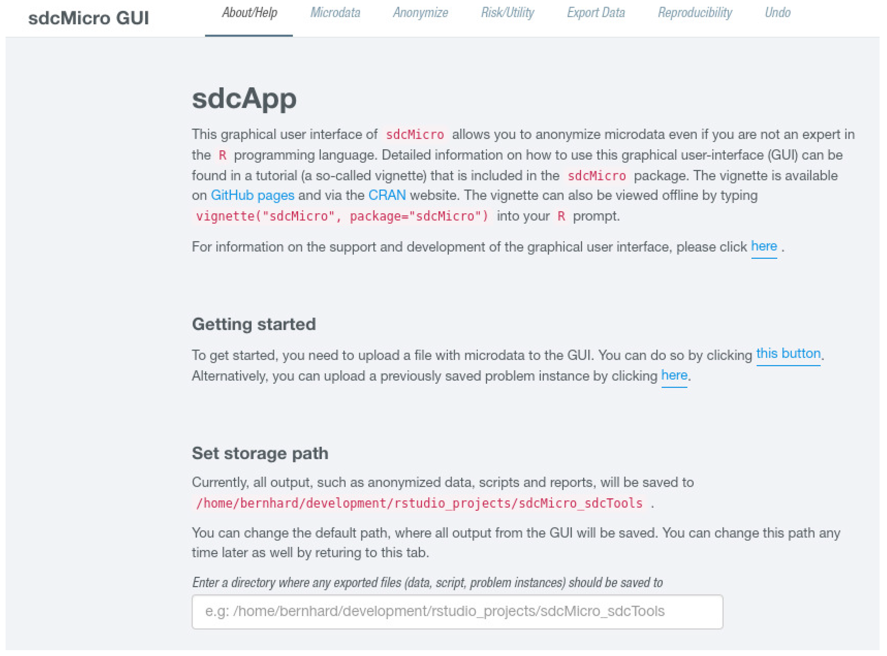
Figure 1 shows parts of the initial GUI once it has been started. The user is presented with some general information on how the interface works. The GUI is organized with “Tabs” that are listed in a navigation bar at the top of the page. The sdcApp() starts by default in the first tab, About/Help, see Figure 1.
The other tabs are named Microdata, Anonymize, Risk/Utility, Export Data, Reproducibility, and Undo, and are discussed in Section 2.2, Section 2.3, Section 2.4, Section 2.5 and Section 2.6. Initially, some of these pages will be empty and their content changes once microdata have been uploaded or an suitable SDC problem has been generated as discussed in Section 2.3. One setting the user can change on this page is the path where all outputs will be saved via the Set storage path text input field. This setting defaults to the current working directory. We now continue to describe the functionality of the GUI in detail.
2.2. Data
Clicking on Microdata at the top of the page gives users the possibility to upload a micro-dataset to the GUI. Once this step has been performed, the page refreshes and quite some features can be selected that allow nonexperts users to easily apply common data manipulation steps (and also to reset them) directly in the GUI before the actual anonymization process is started.
2.2.1. Getting Data into the System
In the tab Microdata, the screen is initially divided in two parts, a left-hand sidebar and a main panel right to it. Users have the option to select from six possibly input formats that can be imported to the system. The choices are to use data objects from the R workspace or to upload separated text files, datasets from R’s binary format or files from other statistical software SPSS, SAS and STATA.
In the main area of the screen, additional options for each file format can be selected. For all but the first choice, a file selector input is shown, where users can select an appropriate file from their hard disk. For the first choice, all data.frame objects from the current R-session are listed as possible choices and can be selected in a drop-down menu. For the other possibilities, other choices are shown depending on the selected data input format. For example, one could change the separator in case of text-separated data, define if characters should be automatically converted to factors, or if variables containing only missing values should be dropped.
After selecting a suitable file and opting to open the file, “sdcApp” tries to import the dataset given the provided options. If the system was not able to successfully read the input, the user is provided with the resulting error message. If the data import was successful, the interface changes. The main part now features an interactive, search-and-sortable table that can be used to check the dataset.
2.2.2. Modify and Analyze Microdata
Also, the left side menu changes once microdata have been successfully uploaded. The menu then contains several options that are provided to modify the microdata. Additionally, a button labeled Reset inputdata is available at the bottom of the sidebar. Clicking this button allows deletion of the current micro-dataset and starting from scratch by uploading a different file.
Table 2 gives a quick overview of the features on this page. In the first column, the name of the link in the sidebar is specified, while, in the second column, a short summary of the specific feature is given. While all the modification steps could also be done before uploading the data, including them in the GUI was done on purpose because the target audience of the GUI are non-R experts which may have problems performing these tasks in pure R.
2.3. Anonymize
Once microdata were uploaded and possibly modified using the methods available as shown in Section 2.2.2, the next required step in the anonymization process is to define a SDC problem instance as explained in the next Section 2.3.1. Once this step has been completed, the dataset can finally be protected and anonymized.
2.3.1. Defining a SDC Problem
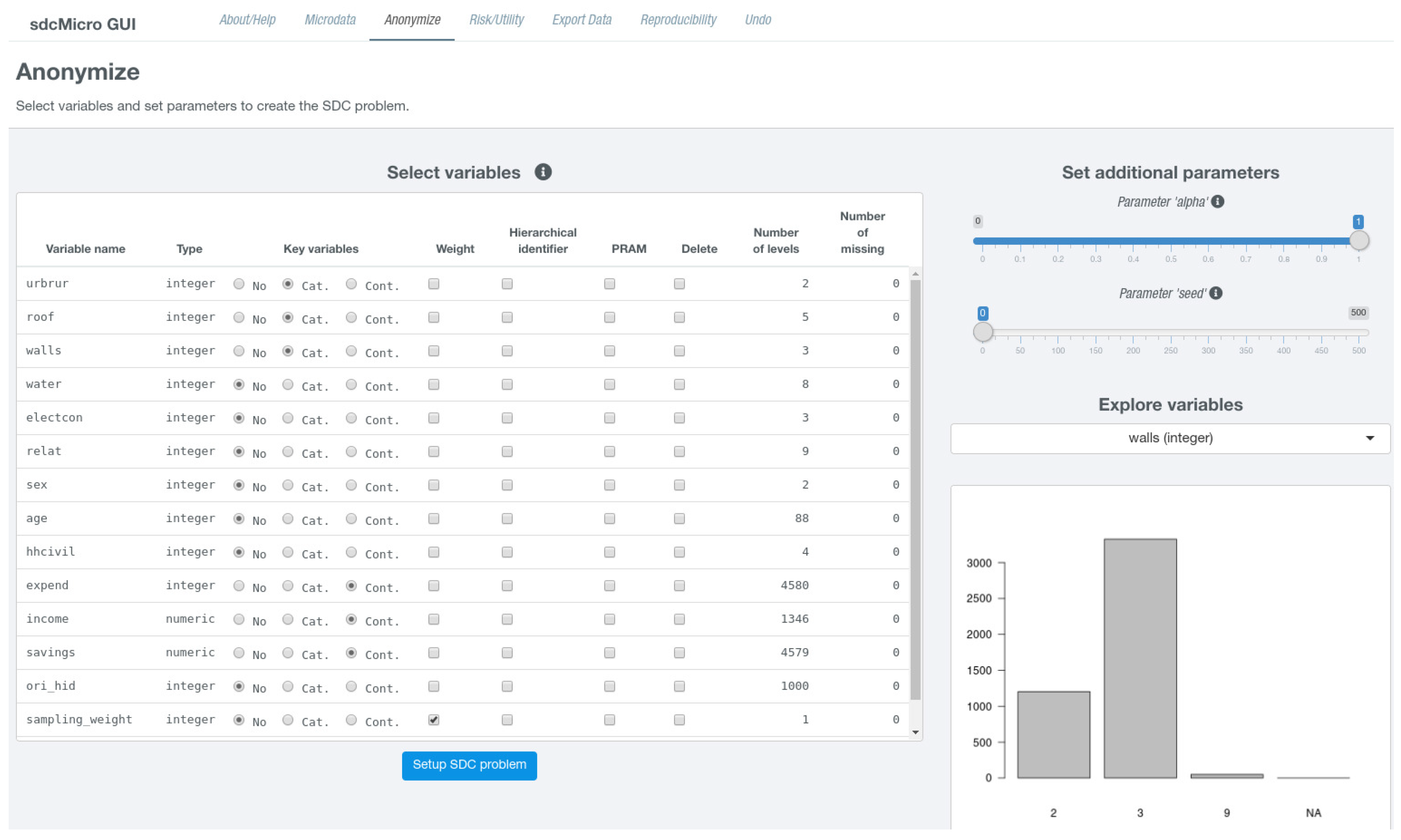
The layout of this page is split into two parts and can be accessed by clicking on Anonymize in the top navigation bar. On the left hand side, an interactive table is shown that needs to be modified in order to define a new problem instance. On the right hand side, the user is given the possibility to select a single variable from the dataset for further exploration, which is shown in Figure 2.
The exploration of variables on the same page is useful to decide which variables should be used as key variables. Below, the variable selection dropdown field, a suitable graph depending on the scale of the selected variable is shown. Below the plot (not shown in Figure 2), summary statistics such as the number of unique values including missing instances of (NA) or a 6-number summary in case of continuous variable are shown while for non-numeric variables a frequency table is displayed. The columns of the interactive table that consists of a single row for each variable from the micro-dataset are listed in Table 3. The page also features two slider inputs labeled Parameter “alpha” and Parameter “seed”. The latter is relevant for specifying an initial start value for the random number generator which is useful if results should be reproducible. The former parameter specifies how sdcMicro should deal with missing values in categorical key variables. Details about this parameter can be found in the help-page of the freqCalc-function.
In column Key variables, radio buttons indicate if a variable should be used as categorical or numerical key variable, which is by default not the case for any variable. However, multiple variables may be uses as categorical and numerical key variables. For columns PRAM, Weight, Hierarchical identifier, and Delete, check boxes are present in the table that are by default not selected and can be enabled by simply clicking on them. Although there can at most be one variable selected as weight variable and variable holding cluster ids, multiple variables may be checked in columns Delete or PRAM. Whenever the table is changed, it is internally checked if all conditions for a successful generation of a new problem instance are fulfilled. In the case that some restrictions are violated, the user is provided visual feedback (either via a popup or red error button) giving information on what needs to be changed. If all checks are passed, a blue button labeled Setup SDC problem appears below the table. Clicking on this button creates the new problem instance. The page then refreshes and the screen layout changes and is divided into two parts. The left sidebar is further subdivided into three sections where different anonymization techniques can be selected. At the bottom of the sidebar there is a button labeled Reset SDC problem that allows deleting the current SDC problem and to create a different instance. The main content either shows results or allows to specify parameters for specific anonymization methods. For all views except for the default view, which summarizes the current problem instance, a right sidebar is displayed in which important measures about the anonymization process as well as risk and data utility measures are shown.
2.3.2. View/Analyze the SDC Instance
The first part of the left navigation sidebar labeled View/Analyze existing sdcProblem allows to select from four different features which are summarized in Table 4.
In the Show Summary-view, the SDC problem is summarized by showing the most important (key) variables of the problem and some statistics, such as the number of suppressed values for each categorical key variable. Furthermore, a table showing the number and percentages of records violating k-anonymity [12,13] for k of 2, 3, and 5 is displayed both for the current problem as well as for the initial problem to which no anonymization procedures have been applied. The user is also presented with information about risk in numerical key variables if any have been defined. In this case, additional tables show the estimated minimal and maximum risk for numeric key variables for both the original and the (possibly) modified continuous key variables as well as measures of information loss. Specifically, measures IL1s [14] and the Difference of Eigenvalues [15] are shown for both the original and (possibly) modified variables. If numeric key variables have been modified, a table containing the six-number summary (identically to the one on the right-hand side below the plot in the page when the problem was defined, see “Defining a SDC problem” in Section 2.3.1) for each the unmodified variable from the micro-dataset and the perturbed variable. Finally, at the bottom all the anonymization procedures that have already been applied are listed.
Clicking on Explore variables allows to explore all variables in their current state. The functionality is exactly the same as it was already described in Modify and analyze microdata (see Section 2.2.2) for original microdata. The only difference being that the analyzed variables are now those from the current SDC problem. The other two features in this section are modifying the SDC problem.
Using Add linked variables it is possible to connect a set of variables to a specific categorical key variable. This variable then serves as a "donor variable. This means that after the anonymization process, all suppressions of the donor variable will be transferred to the variables linked to it.
Sometimes it is useful to create a new random identifying variable. Therefore, this task can also be performed within the GUI by clicking on the link “Create new IDs”. After specifying a new variable name and optionally a variables that serves as grouping variable (the new variable will have random, but common values for each value of the grouping variable), the new variable can be created by clicking on a button labeled Add new ID variable which appears at the bottom of the page. After the variable has been created, the page switches to the Show Summary view.
2.3.3. Anonymization of Categorical Data
The second subsection of the left sidebar labeled Anonymize categorical variables allows applying anonymization methods to categorical key variables. The available methods are listed in Table 5.
Selecting Recoding allows reducing the level of detail of categorical key variables by combining levels into a new, common category which can optionally be renamed; it is also possible to add missing values to the newly generated category. Once the re-coding is done, the page refreshes and the content in the right sidebar like the number of observations violating k-anonymity was updated.
It is very common feature that a safe micro-dataset features k-anonymity [12,13]. This feature specifies that each combination of the levels of the categorical key variables occurs at least k times in the data. Choosing k-Anonymity allows creating a k-anonym dataset for all or (independently) for given subsets of the categorical key variables. The latter approach is useful if the number of categorical key variables is large. Furthermore it is also possible to set different values of k for the subsets. The algorithm works by setting specific values in key variables to missing (NA). Users can also rank variables by importance to be selected as variable in which values should be removed. This allows to specify variables that are deemed so important that no missing values should be introduced by the algorithm. By default the key variables are ordered in a way that the variables with the most number of levels are most likely to be selected as variable in which suppressions are introduced. The implementation of the algorithm also allows to apply the method independently on groups defined by a stratification variable. If the user opts for this approach, a variable defining the grouping needs to be selected from a drop-down menu. For any way, the value of k is typically set using slider inputs. Once the user has finished setting the parameters, an action button appears at the bottom of the page. Clicking this button starts the process to establish k-anonymity which might take some time. While the algorithm runs, a progress bar is displayed. Once the calculation has finished, the page refreshes and the right sidebar was updated. Users should especially have a look at the first table in which the number of suppressions for each key variable is shown. Also, the section k-anonymity in the sidebar is updated.
Post-randomization (PRAM) [16] is a statistical process that possibly changes values of a variable given a specific transition matrix. In the GUI, PRAM can be applied in two different ways by either choosing PRAM (simple) or PRAM (expert). In both cases, at least one variable needs to be selected that should be post-randomized. We note that only those variables can be selected that have been defined as being suitable for post-randomization when defining the SDC problem as discussed in Section 2.3.1. We note that it is possible to select a single stratification variable. If this is the case, the post-randomization procedure is performed independently for each unique value of the grouping variable. The definition of the transition matrix is different for the “simple” and the “expert” mode. In PRAM (simple), two parameters must be specified using slider inputs. pd refers to the minimum diagonal values in the (internally) generated transition matrix. The higher this value is, the more likely it is that a value stays the same and remains unchanged. Parameter alpha allows to add some perturbation to the calculated transition matrix. The lower this number is, the less perturbed the matrix will get. This information is also displayed when hovering over question mark icons next to the slider inputs. In PRAM (expert), the user needs to manually create a transition matrix by changing cell values of an interactive table. The diagonal values of the table are by default 100 which results in a transition matrix in which no value would be changed. For any given row, the numbers are defined as percentages that the current value of the selected variable (the row name) changes to the value specified by the respective column name. The user needs to make sure that the sum of values in each row equals 100. If this is not the case, a red button appears below the table, giving instant feedback that the table needs to be modified. Values in specific cells may be changed by clicking into the cell and entering a new values. If the inputs were specified correctly, a button appears at the bottom of the page. Pressing this button applies PRAM using the defined parameters. Once finished, the page refreshes and in the right sidebar a section called PRAM summary either appears or is extended. In this part of the right sidebar, for each variable that has been post-randomized the number and percentages of value changes are listed.
Clicking on Suppress values with high risks makes it possible to set values for the most risky records to NA. It is required to select a categorical key variable and specify using a slider input an appropriate threshold value which will be used to identify the “risky” records. These records are defined as those having an individual re-identification risk [17] larger than the selected threshold value. The threshold can be changed by updating the slider. Below the inputs, a histogram displaying the distribution of the individual risk values is shown. In this graph, a vertical black line representing the current value of the threshold is plotted. Finally, at the bottom of the page, a button with a dynamic label is shown. The label contains the number of records that would be suppressed as well as the selected variable. Once the button is pressed, records in the selected variable whose individual risks are above the threshold are set to NA. The view then changes to the Show summary view.
2.3.4. Anonymization of Continuous Data
The third section in the left-hand sidebar shows the methods that can be applied to numerical (key) variables. Table 6 summarizes the possible choices.
We note that only the first choice (Top/Bottom coding) is always listed; the remaining choices only appear if at least one variable has been set as continuous key variable when defining the problem, as discussed in Section 2.3.1.
Selecting Top-/Bottom-Coding enables the user to replace values that are above (top-coding) or below (bottom-coding) a threshold with a different number, which is typically the threshold itself. In the GUI, the user needs to select a variable from a drop-down field that should be re-coded. This field only allows to select continuous variables in order to prevent the application of the method to categorical variables. Then it must be set if top- or bottom coding should be performed using a radio button input field. Furthermore, two numbers—the threshold value and the replacement value—must be set. To help users find suitable threshold values, a box plot showing the distribution of the currently selected variable is shown below the input controls. After all inputs have been set, additional elements appear between the input fields and the box plot. The first additional element is a text stating how many of the values would be replaced as well as the corresponding percentage. Below this information, a button appears. Once this button is pressed, the values are replaced according to the current settings and the page refreshes. The box plot is updated as well as the right hand sidebar. If the selected and re-coded variable was defined as a numeric key variable, the values referring to risk in numerical key variables and information loss measures change in the sidebar.
Microaggregation [18] is a method in which records are grouped based on a proximity measure of variables of interest. In a second step, for each group, a summary statistic (aggregate value), which is typically the arithmetic mean, is computed and then released for all records in the group, instead of the original, individual record values. This method reduces the variation of a continuous key variable and additionally protects against (direct) matching. It also can be interpreted as k-anonymity for continuous variables. In sdcMicro, non-cluster-based and cluster-based methods are distinguished. Users can choose from a total of eight non-cluster-based and four cluster-based methods. The grouping can also be can be nonrobust (for example, the default algorithm Maximum Distance to Average Vector (MDAV) [3]) or robust such as the Robust Maximum Distance (RMD) algorithm [19].
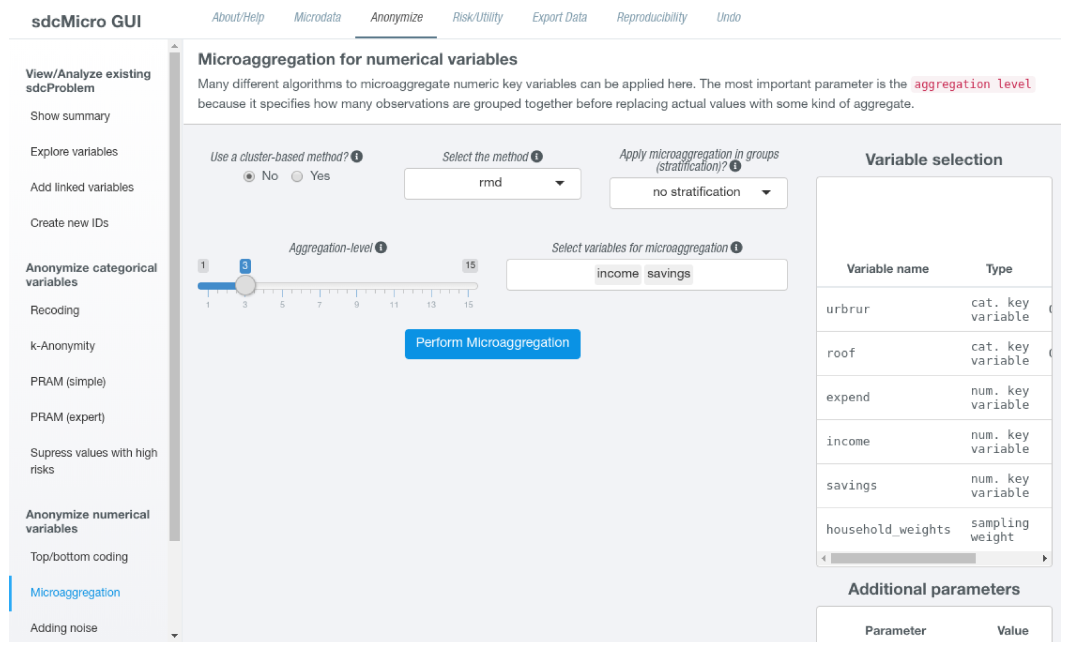
If the users chooses to apply microaggregation to numeric key variables, the first choice is to select one of the available methods from a drop-down menu. The user also needs to specify an aggregation level using a slider input. This value refers to the size of the groups that will be formed by the algorithm. Further options that can be made include the selection of a subset of numerical key variables for which should be microaggregated (by default, all key variables will be used) or if the algorithm should be applied independently given the characteristics of a stratification variable that needs also be chosen in this case. Figure 3 features a screen shot how the RMD algorithm may be specified for some continuous key variables without stratification for a group size of 3.
Additionally, question mark icons are shown next to most input fields. By hovering over these icons, additional information is shown in a pop-up window, which will facilitate users to find appropriate parameter settings. For some methods, several additional inputs are shown. For example, when using cluster-based methods, it is possible to select the clustering algorithm (such as “kmeans”, “cmeans”, or “bclust”) as well as possible data transformations (“log”, “box-cox”, or “none”) that should be applied before the cluster algorithm is applied. For some non cluster-based methods, it is possible to choose the aggregation statistics (such as the mean or the median). Once all required options have been set, an action button appears below all inputs. Clicking on this button performs the microaggregation of the selected variables according to the options that have been set. As the computation might take some time, on the bottom right screen, a progress bar showing that the process is running appears. Once the algorithm has finished, the page updates and the “Show summary” page is displayed. On this page, all measures depending on numerical key variables have been recomputed and show current values.
Another popular way to mask numerical variable is to overlay original numbers with a stochastic noise distribution that has typically a mean of 0. Selecting Adding Noise allows to modify numerical key variables with noise. Users can select one or more numerical key variable from a input field which is by default empty. If it is left empty, all numerical key variables will be perturbed. Next to the variable selection field, a single specific algorithms needs to be selected. While some of the algorithms (e.g., “additive”) add noise completely at random to each variable depending on its size and standard deviation, other methods are more sophisticated. Algorithms “correlated” and “correlated2” [20] try to preserve the covariance structure of the input variables. Method “ROMM” [21] is an implementation of the Orthogonalized Matrix Masking method) and algorithm “outdect” [19] adds noise only to outliers. These outliers are identified by univariate and robust multivariate procedures based on a robust Mahalanobis distance which is computed by the MCD estimator [22].
Below these inputs, the amount of perturbation needs to be specified by changing the value of a slider input. This input is dynamically labeled depending on the previous choice of the method. Since the parameterization for the different methods is different, this slider has different default values and different ranges depending on the choice of the method. If all options have been set, pressing a button that is shown at the bottom of the page finally applies the stochastic noise to the selected variables. Once the algorithm finished, the page view changes to the Show summary page, where again all relevant measures were recalculated.
The last method that can be applied to numerical key variables is rank swapping [23]. The main idea of this algorithm is to swap values within a given range so that the correlation structure of the original variables is (mostly) preserved and some perturbation is added to the variables. After specifying the numerical key variables to which the algorithm should be applied, the parameters for the procedure needs to be specified using five different slider inputs. Two sliders are used to define percentages of values to be bottom- or top-coded before the algorithm starts, which allows to deal with outlying observations. The sliders named “Subset-mean preservation factor” and “Multivariate preservation factor” allow further fine-tuning of the algorithm. The first one defines how the maximum percentage means before and after the perturbation are allowed to differ, while the second slider specifies a limit on how much correlations between non-swapped and swapped variables are allowed to differ. Using the fifth and last slider allows defining a maximum distance relative to their ranks, which needs to be fulfilled for two records to be eligible for swapping. For details on the impact of these parameters, please see the help page for the rankSwap-function ?rankSwap. After all options were set, clicking on an action button at the bottom of the page starts the swapping procedure. Once finished, the page view changes as already previously described to the summary view where all the relevant statistics are shown and can be analyzed.
2.4. Risk/Utility
Anonymizing microdata is typically an interactive process. Methods are applied with specific parameter settings, and then the resulting dataset needs to be checked as applying disclosure limitation techniques and data utility are obviously tied together. The more impact the anonymization measures have and thus, the more anonymized the microdata are, the less useful it might be for the target audience. It is therefore a difficult task to balance risk and data utility. Often it is the case that it turns out that specific parameter settings need to be changed after having a look at data utility or risk measures. The GUI easily allows reverting the last method by clicking on a button that can be found by clicking on tab labeled Undo in the top navigation panel. If this is done, different parameter settings or methods can be applied and the results can be analyzed.
To analyze the current state of the anonymized data and compare it with the unprotected original microdata, clicking on tab Risk/Utility leads to a page where risk and utility measures as well as visualizations and tabulations are presented. This page is again subdivided into three parts featuring a left-sided navigation bar, a centered main part and a right-sided info panel in which two tables are shown. The first table, labeled Variable selection lists the categorical and numerical key variables. Additionally (if present), the variables selected to be possibly post-randomized as well as the variables holding sampling weights or cluster ids are shown. The second table labeled Additional parameters shows the number of records as well as the choice of parameters for the random-seed initialization and parameter alpha, already discussed in Section 2.3.1. The left sidebar contains all the features that can be selected and is divided into three section labeled Risk measures, Visualizations, and Numerical risk measures that are discussed in Section 2.4.1, Section 2.4.2 and Section 2.4.3. Clicking on a specific link in the navigation bar changes the view of the centered content in which either results are displayed or the user can interactively specify additional parameters. We note that the current selection is colored differently than the rest so that it is easy to see which selection is active.
2.4.1. Risk Measures
This part deals with information based on the risk scenario defined by the categorical key variables. Table 7 summarizes the choices that can be made.
Selecting Information of risks by default displays the number and percentages of observations that have a higher individual re-identification risks [17] than the main part of the other records. This information is shown for both the initial as well as the anonymized dataset. The individual re-identification risk is computed based on the defined categorical key variables and reflects both the frequencies of the keys in the dataset and takes individual sampling weights into account if such have been specified. A record is said to have a re-identification risk different from the main part of the data if its personal re-identification risk is either larger than the median plus two times the Median Absolute Deviation of the distribution of all individual risks (a robust measure) or if it is deemed large. Furthermore, the number and percentage of expected re-identifications based on the individual risk approach for the original and modified dataset are displayed.
At the top of the page, a group of radio buttons allows to change the results that will be shown. Selecting Risky observations allows filtering records in the anonymized dataset, depending on a threshold for the individual re-identification risk that can be selected using a slider input. Below this slider, the number and percentages of observations with individual re-identification risks larger than the currently specified threshold are shown and a table showing the units having larger individual risks than the current threshold are shown. The table contains categorical key variables as well as its individual risk value and numbers of fk and Fk that specify how often the combination of characteristics of the key variable for the given unit occurs in the sample (fk) and how often the combination is estimated to occur in the population (Fk).
Selecting Plot of risk using the radio button input field leads to two plots being shown. Both plots show histograms of individual re-identification risks. The upper plot shows the risks from the original, unmodified microdata while the second graph is based on the current state of the dataset and takes all previously applied SDC methods into account.
The second option in the left-sided navigation bar—Suda2 risk measure–allows the user to apply the SUDA algorithm [24]. This algorithm can be used to search for Minimum Sample Uniques (MSU) in the data given the current set of categorical key variables. The algorithm looks at those records that are unique in the sample (sample uniques) and furthermore checks if any of these sample uniques are also special uniques. Special uniques are defined as records for which also a subset of the categorical key variables are sample unique. This algorithm can only be applied if the current problem instance has three or more categorical key variables specified. If the prerequisites are fulfilled, the user needs to choose a value for parameter disFraction by modifying a slider input field. This parameter refers to the sampling fraction for the simple random sampling or the common sampling fraction for stratified sampling used by the algorithm. After pressing an action button, the suda scores are computed and two tables are shown in the center pane. The first table summarizes the obtained suda scores. It shows for 0 and eight intervals the number of records having scores belonging to the corresponding category. The second table shows, for each categorical key variable, how much of the total risk is contributed to by each of the categorical key variables. Additionally, a further button is shown that enables to restart the computation of this risk measure using a different value for the sampling fraction parameter.
The last option in this group allows computing of the l-diversity risk measure of sensitive variables [25] by clicking on link l-Diversity risk measure. A dataset satisfies l-diversity if, for every combination of the categorical key variables, there are at least l different values for each of the sensitive variables. The statistics refers to the value of l for each record. To calculate this risk measure, the user needs to select at least one sensitive variable which should be evaluated using a select input field from which all variables except the categorical key variables can be chosen. Furthermore, a value for l needs to be selected. Clicking on an action button computes the l-diversity risk measure and the content of the page changes. It then displays a table that contains - for each selected sensible variable - the five-number summary of the calculated l-diversity measure. Further below, all records violating l-diversity are displayed in an interactive table if there is at least one record violating l-diversity. As for the Suda2 measure discussed above, a button is also shown that allows to reset the parameter choices and to recompute the risk measure with a different value of l or other sensitive variables.
2.4.2. Visualizations
The second block in the left-hand sidebar allows to either compare current key variables in the original and anonymized dataset graphically or using summary statistics presented in tables. It is also possible to view measures of information loss based on re-coding and display the number of observations violating k-anonymity for arbitrary values of k. Table 8 summarizes the possibilities.
The first two choices Barplot/Mosaicplots and Tabulations allow to compare the distribution of categorical key variables. For both cases, the user hast to select one or two categorical key variables from drop-down input fields in which only the categorical key variables can be selected. For the former case, two plots appear below the inputs, whereas in the later case, two tables are shown next to each other below the select input fields. Both the graphs and the tables are automatically updated if the selection of key variables changes.
If only one variable is specified and the value of the second variable selection input field is None, the user is either shown a bar plot showing the number of occurrences for each level of the input variable or a simple frequency table showing exactly the same information. In case two variables have been selected, either a mosaic plot or a cross-tabulation of the two selected variables for both the original and the anonymized variables is shown.
Selecting Information loss shows measures of information loss that are due to re-coding (or rather combining) levels of categorical key variables, thus removing information from the data. Here, users are presented with an interactive table that can be sorted by clicking on the small arrow signs that are shown next to the column names. The table includes, for each categorical key variable, the name of the key variable, the number of levels, and the mean and minimum size of categories for the original and the modified variables.
The next feature is to find out how many records in the anonymized dataset violate k-anonymity for different choices of parameter k. By clicking on Obs violating k-Anon, the user is presented with a slider input that refers to parameter k. Dragging the slider with the mouse or changing the value of the slider with the arrow keys on the keyboard leads to a recalculation of the number and percentage of observations that violate the k anonymity measure. This information is printed on the screen below the slider. Additionally, a table listing all the observations in the dataset violating k-anonymity is shown. For these observations, the interactive table contains all categorical key variables as well as the estimated individual risks (in column risk) as well as parameters fk and Fk as discussed in Section 2.4.1.
2.4.3. Numerical risk measures
The third block in the left navigation bar in the Risk/Utility tab provides information on risk and data utility for numerical key variables. The features are summarized in Table 9.
In Compare summary statistics, it is possible to compare the distribution of the numerical key variables defined in the current SDC problem between the original and the anonymized data. This comparison is optionally also possibly for each level of a categorical key variable. To start, a numerical key variable needs to be selected from a drop-down field. Next to this input, another drop-down field is shown from which optionally may select one of the categorical key variables. Once the selections have been made, below the input fields some some important values such as the Pearson correlation coefficient using pairwise complete information, the standard deviations as well as the interquartile range and of the numerical key variable in the original and the anonymized dataset is displayed in a section named Measures.
Below this information, two tables are presented where the first refers to the original and the second to the anonymized data. Both tables contain the extreme values, arithmetic mean and median as well as as the 5%-, 25%-, 75%-, and 95%-quantiles. In the case where a categorical variable has been chosen, these summary statistics are calculated for each level of the selected categorical key variable; otherwise, the summary statistics are computed over the entire dataset. We note that since the levels of the categorical key variables might differ between original and anonymized dataset, it is not possible to show this information in a single table.
If the link Disclosure Risk is chosen, it is possible to check on the estimated disclosure risk for the defined numerical key variables. The measure can be interpreted in the following way. In the original, unmodified data that has been used to create the SDC problem instance, the risk for the numeric key variables is assumed to be between 0% and 100%. The more data anonymization techniques such as microaggregation or adding noise are applied to the data, the less the upper bound of the risk will be. So users can compare the estimated upper bound of the risk for numerical key variables in the anonymized data and compare on how much it has reduced from the initial value of 100%. We note that the larger the deviations from the original data are, the lower the upper risk bound will be. However, this has of course also an impact on data utility measures that can be assessed from the menu button Information loss, which is the last choice in this tab.
Clicking on Information loss, two measures of information loss, IL1s [14], and a robust measure based on differences in eigenvectors [15] for numerical key variables are shown. Generally, the more the numerical key variables are modified or rather anonymized, the higher the information loss values for both measures. We also note that information loss and the disclosure risk for numerical variables as discussed previously are always a trade of which need to be balanced.
2.5. Export Data
Clicking on the link labeled Export data in the top navigation bar changes the GUI and shows a left hand sidebar as well as a main content area. In this part of the application, users can either save a microdata file using the current state of the defined SDC problem into various formats or to create and save a report summarizing the anonymization process to the hard disk. If no SDC problem has been specified, the user is informed of the need to create or to upload a previously exported SDC problem instance first. Saving or importing a problem instance can be done in tab Reproducibility as discussed in Section 2.6.
Selecting Anonymized Data, the microdata available at present in the active SDC problem after applying all disclosure limitation techniques can be saved to disk. At the top of this page, an interactive, sortable, and browsable table containing the data that will be written to a file is shown to allow for a final check of the data. The variables can be sorted by clicking on the small arrows next to the variable names on top of the table. At the bottom of the table, users find a dynamic pagination field that allows users to jump to a given page of the table which is useful if the dataset consists of a large number of observations. Below the table, two sets of radio buttons are shown that allow to select the file format in which the result should be exported to and to define, if the order of the rows should be randomized.
Currently, five different output formats can be specified. Using functionality from R package haven [26], it is possible to create output for statistical software packages SAS, SPSS, and STATA, as well as separated plain text files and files in R’s own binary format. For some output formats, additional inputs appear that allow, for example, to specify the field- and decimal separator in case of text-separated output or the specific STATA file-format version in case a dta-file suitable for STATA should be created.
The second radio control input allows randomizing the order of observations in the dataset. If Randomization at record level is selected, the records of the dataset are randomly changed. In the case where a household or cluster variable was defined when setting up the SDC problem, two additional options are displayed. Selecting Randomize by hierarchical identifier randomizes the values of this identification variable across the dataset. If the user opts to choose Randomize by hierarchical identifier and within hierarchical units, not only are the values of the household identification variable randomly changed but also the order of records within the clusters will be permuted. By default however, no randomization of the order of statistical units is applied and the current order remains. Once all settings are made, at the bottom of the page a action button is shown. Clicking this button finally creates a file using the specified parameters in the destination folder that has been set in the About tab discussed in Section 2.1.
The second option in this tab allows the creation of a report summarizing the anonymization process, which can be achieved by clicking on Anonymization Report. Here, the user can select the type (internal or external) of the report by setting the desired value using radio buttons. The default choice results in a rather long and quite detailed report whereas the alternative choice only gives a very broad overview about which disclosure limitation techniques have been applied and some basic statistics on the resulting micro-dataset. Clicking on a button at the bottom of the page creates the report using functionality from R packages brew [27] and knitr [28] and saves it as an html-file in the destination folder that has been specified in the About tab as described in Section 2.1.
2.6. Reproducibility
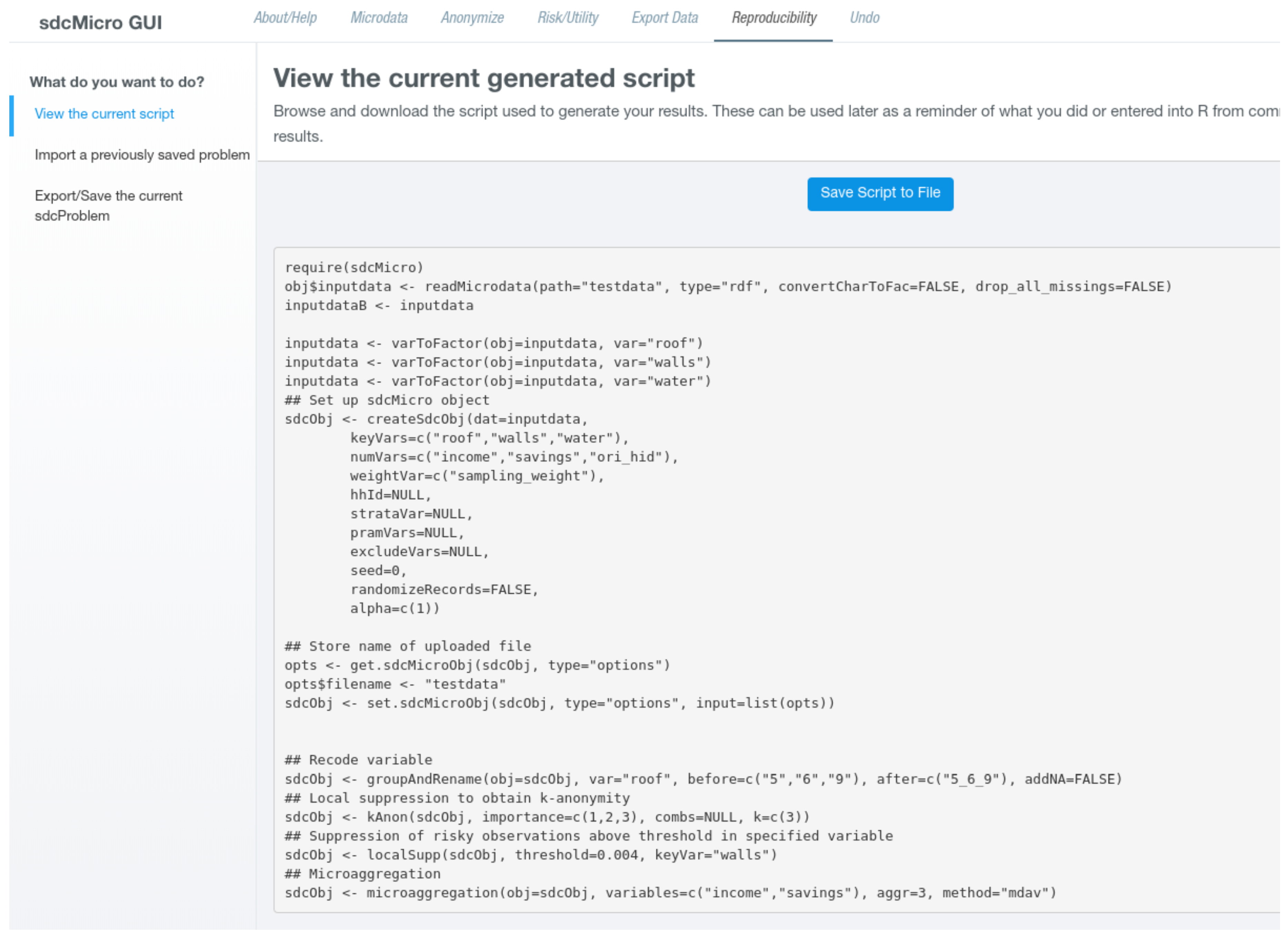
In this tab, users are presented with information which allows to completely reproduce the anonymization steps in the command line interface of sdcMicro. If a SDC problem instance has been defined, the page shows again a left-navigation bar and a main content area. Selecting View/Save the current script shows the R-code, which is required to reproduce the current state which is shown in a text-area input field. Above, a action button is shown that allows to download the code as an .R-file as it is shown in Figure 4.
The code shown here could be run in sdcMicro directly with the only limitation being that the file path when uploading microdata files is relative to the fileInput()-functionality of shiny which gives no way to return the path of the uploaded file on the local disk. For full reproducibility, users may need to adjust the path listed in the script before running it.
Another possible choice is to select Import a previously saved sdcProblem from the left-sidebar. In this case, a file input selector appears. Clicking on Browse allows to search the local hard disk for a previously exported problem instance. The file chooser only allows to upload .rdata-files to minimize possible mistakes. Once the file has been located and the Open button was pressed, the system tries to load the file. Internally, some checks are made and if the import was successful, the GUI shows the overview of the uploaded SDC problem as described in Section 2.3.2. If the data import was unsuccessful, the user is instead shown an error message and a button labeled Try again!.
The last possible choice in the navigation menu on this page is Export/Save the current sdcProblem where, if a SDC problem has been defined, a button labeled Save the current problem is shown along with some further explanations. Clicking this button saves the entire current problem which includes all GUI-related meta data to a file on the hard disk in the current destination folder.
3. Conclusions
In this work we have presented the interactive, web-based GUI of sdcMicro that also allows nonexperts in R to perform statistical data anonymization of microdata. In this work we showed that the GUI is not restricted to apply disclosure limitation techniques but rather facilitates the entire anonymization process from uploading and preparing microdata as discussed in Section 2.2.1 and Section 2.2.2, setting up and defining a problem instance that is suitable for sdcMicro, as shown in Section 2.3.1, to interactively applying disclosure limitation techniques to the data (Section 2.3.3 and Section 2.3.4) and analyzing the impact of the methods in terms of a risk- and data utility assessment as presented in Section 2.4. The dataset to be anonymized can (but not necessarily must) have a complex hierarchical structure (e.g., persons in households), could be sampled with a complex sampling design, can include continuous and categorical scaled key variables (quasi-identifiers) and can include stratification variables. Using such variables, it is possible to apply several methods to each strategy independently. Once these complexities are specified in the problem instance, these specialties are automatically considered for all internal risk-, utility and anonymization computations. The possibility of setting up complex problem instances goes much beyond what other tools, such as Arx, PARAT, OpenAnonymizer, SECRETA, Amnesia, Cornell Anonymization Toolkit, and TIAMAT, offer.
Finally, facilities are provided to not only save the final micro-dataset to disk, but also to create summary-reports that give an overview of the anonymization process (Section 2.5). Even though the GUI is meant to be interactive in the sense that users are changing values and parameters using the mouse or the keyboard, it has been made sure that the process itself is reproducible. The R-code that is required to reproduce the anonymized can be viewed and downloaded as shown in Section 2.5; it is also possible to export and import the current state of the GUI.
Throughout the GUI, question mark icons are displayed that contain additional useful information of users once they hover over the icons with their mouse. The Undo-feature explained in Section 2.4 was also proven useful because it allows easily reverting the application of a method if the specific parameter settings showed that the achieved improvement in terms of risk reduction were too low or the impact on the usefulness of the data measured in terms of data utility was too high. Method-richness, reproducibility and features like this Undo button and extensive reporting facilities as well as instant changes and display of risk, utility and data are only implemented in sdcApp and not (or only very limited) available in tools like -Argus.
sdcMicro and its GUI are still actively developed and maintained, and feature requests or reporting issues via the issue tracker at https://github.com/sdcTools/sdcMicro/issues are welcome for further improving the software.
Author Contributions
Funding
The development of the shiny-based GUI was funded by the World Bank Group (http://www.worldbank.org) and the Department for International Development DfID (https://www.gov.uk/government/organisations/department-for-international-development).
Conflicts of Interest
The authors declare no conflict of interest.
Abbreviations
The following abbreviations are used in this manuscript.
| GUI | Graphical User Interface |
| SDC | Statistical Disclosure Control |
| CRAN | Comprehensive R Archive Network |
| NA | Not Available (symbol in R) |
| PRAM | Post-Randomization |
| MSU | Minimum Sample Uniques |
References
- Templ, M.; Kowarik, A.; Meindl, B. Statistical Disclosure Control for Micro-Data Using the R Package sdcMicro. J. Stat. Softw. 2015, 67, 1–36. [Google Scholar] [CrossRef]
- Templ, M. Statistical Disclosure Control for Microdata; Springer International Publishing: Basel, Switzerland, 2017; ISBN 978-3-319-50270-0. [Google Scholar] [CrossRef]
- Hundepool, A.; De Wolf, P.-P.; Bakker, J.; Reedijk, A.; Franconi, L.; Polettini, S.; Capobianchi, A.; Domingo-Ferrer, J. mu-Argus User’s Manual version 5.1; Statistics Netherlands: The Hague, The Netherlands, 2014. [Google Scholar]
- Dai, C.; Ghinita, G.; Bertino, E.; Byun, J.W.; Li, N. TIAMAT: A Tool for Interactive Analysis of Microdata Anonymization Techniques. PVLDB 2009, 2, 1618–1621. [Google Scholar] [CrossRef]
- Poulis, G.; Gkoulalas-Divanis, A.; Loukides, G.; Skiadopoulos, S.; Tryfonopoulos, C. SECRETA: A System for Evaluating and Comparing RElational and Transaction Anonymization algorithms. In Proceedings of the 17th International Conference on Extending Database Technology (EDBT 2014), Athens, Greece, 24–28 March 2014; pp. 620–623. [Google Scholar]
- Amnesia: A flexible Data Anonymization Tool that Transforms Relational and Transactional Databases to Dataset Where Formal Privacy Guaranties Hold. Available online: https://amnesia.openaire.eu/index.html (accessed on 30 August 2019).
- Cornell Anonymization Toolkit: Designed for Interactively Anonymizing Published Dataset to Limit Identification Disclosure of Records Under Various Attacker Models. Available online: https://sourceforge.net/projects/anony-toolkit (accessed on 30 August 2019).
- Prasser, F.; Kohlmayer, F. Medical Data Privacy Handbook; Chapter Putting Statistical Disclosure Control into Practice: The ARX Data Anonymization Tool; Springer: Cham, Switzerland, 2015. [Google Scholar]
- Nergiz, M.; Atzori, M.; Clifton, C. Hiding the Presence of Individuals from Shared Databases. In Proceedings of the 2007 ACM SIGMOD International Conference on Management of Data, Beijing, China, 11–14 June 2007; ACM: New York, NY, USA, 2007; pp. 665–676. [Google Scholar] [CrossRef]
- Chang, W.; Cheng, J.; Allaire, J.; Xie, Y.; McPherson, J. Shiny: Web Application Framework for R, R Package Version 1.3.2; 2019. Available online: https://CRAN.R-project.org/package=shiny (accessed on 9 September 2019).
- Templ, M.; Petelin, T. A Graphical User Interface for Microdata Protection Which Provides Reproducibility and Interactions: the sdcMicro GUI. Trans. Data Priv. 2009, 2, 207–223. [Google Scholar]
- Samarati, P.; Sweeney, L. Protecting Privacy when Disclosing Information: k-Anonymity and Its Enforcement through Generalization and Suppression; Technical Report SRI-CSL-98-04; Computer Science Laboratory, SRI International: Menlo Park, CA, USA, 1998. [Google Scholar]
- Sweeney, L. k-anonymity: A model for protecting privacy. Int. J. Uncertainty Fuzziness Knowl.-Based Syst. 2002, 10, 557–570. [Google Scholar] [CrossRef]
- Mateo-Sanz, J.; Sebé, F.; Domingo-Ferrer, J. Outlier Protection in Continuous Microdata Masking. In Privacy in Statistical Databases; Lecture Notes in Computer Science; Springer: Berlin/Heidelberg, Germany, 2004; Volume 3050, pp. 201–215. [Google Scholar]
- Templ, M.; Meindl, B. Robust Statistics Meets SDC: New Disclosure Risk Measures for Continuous Microdata Masking. In Privacy in Statistical Databases; Domingo-Ferrer, J., Saygın, Y., Eds.; Springer: Berlin/Heidelberg, Germany, 2008; pp. 177–189. [Google Scholar]
- Gouweleeuw, J.; Kooiman, P.; De Wolf, P. Post-randomization for statistical disclosure control: Theory and implementation. J. Off. Stat. 1998, 14, 463. [Google Scholar]
- Franconi, L.; Polettini, S. Individual Risk Estimation in mu-Argus: A Review. In Privacy in Statistical Databases; Domingo-Ferrer, J., Torra, V., Eds.; Springer: Berlin/Heidelberg, Germany, 2004; pp. 262–272. [Google Scholar]
- Gower, J. A General Coefficient of Similarity and Some of Its Properties. Biometrics 1971, 27, 857–871. [Google Scholar] [CrossRef]
- Templ, M.; Meindl, B. Robustification of Microdata Masking Methods and the Comparison with Existing Methods. In Privacy in Statistical Databases; Domingo-Ferrer, J., Saygın, Y., Eds.; Springer: Berlin/Heidelberg, Germany, 2008; pp. 113–126. [Google Scholar]
- Brand, R. Microdata Protection through Noise Addition. In Inference Control in Statistical Databases; Lecture Notes in Computer Science; Springer: Berlin Heidelberg, Germany, 2002; Volume 2316, pp. 97–116. [Google Scholar]
- Ting, D.; Fienberg, S.; Trottini, M. Random Orthogonal Matrix Masking Methodology for Microdata Release. Int. J. Inf. Comput. Secur. 2008, 2, 86–105. [Google Scholar] [CrossRef]
- Rousseeuw, P. Least Median of Squares Regression. J. Am. Stat. Assoc. 1984, 79, 871–880. [Google Scholar] [CrossRef]
- Moore, R. Controlled Data-Swapping Techniques for Masking Public use Microdata Sets; Statistical Research Division Report Series; US Census Bureau: Suitland, MD, USA, 1996; pp. 96–104.
- Manning, A.; Haglin, D.; Keane, J. A recursive search algorithm for statistical disclosure assessment. Data Min. Knowl. Discov. 2008, 16, 165–196. [Google Scholar] [CrossRef]
- Machanavajjhala, A.; Kifer, D.; Gehrke, J.; Venkitasubramaniam, M. L-diversity: Privacy Beyond K-anonymity. ACM Trans. Knowl. Discov. Data 2007, 1. [Google Scholar] [CrossRef]
- Wickham, H.; Miller, E. Haven: Import and Export ‘SPSS’, ‘Stata’ and ‘SAS’ Files, R package version 2.1.1; 2019. Available online: https://CRAN.R-project.org/package=haven (accessed on 9 September 2019).
- Horner, J. Brew: Templating Framework for Report Generation, R Package Version 1.0-6; 2011. Available online: https://CRAN.R-project.org/package=brew (accessed on 9 September 2019).
- Yihui, X. Dynamic Documents with R and knitr, 2nd ed.; Chapman and Hall/CRC: Boca Raton, FL, USA, 2015; ISBN 978-1498716963. [Google Scholar]
Figure 1.
AboutHelp tab: Help-page of sdcApp after it has been started.

Figure 2.
Defining a problem instance: on the left hand side important (key) variables can be defined, while a suitable graphic on the right hand side helps to identify suitable variables.
Figure 2.
Defining a problem instance: on the left hand side important (key) variables can be defined, while a suitable graphic on the right hand side helps to identify suitable variables.

Figure 3.
Screen to set up microaggregation in the GUI.

Figure 4.
View/analyze the required code to reproduce the current state.


Table 1.
List of methods that can be accessed via a GUI. Circles indicate only limited potentiality/support.
Table 1.
List of methods that can be accessed via a GUI. Circles indicate only limited potentiality/support.
| Method/Software | μ-Argus 4.2 | Arx | sdcApp > 1.1.0 |
|---|---|---|---|
| frequency counts | ✔ | ✔ | ✔ |
| individual risk (IR) | ✔ | ✔ | |
| IR on households | ✔ | ✔ | |
| l-diversity | ✔ | ✔ | |
| t-closeness, δ-presence | ✔ | ||
| suda2 | ✔ | ||
| global risk (GR) | ✔ | ✔ | |
| re-coding | ✔ | ✔ | ✔ |
| local suppression | ✔ | ✔ | ✔ |
| swapping | ✔ | ✔ | |
| pram | ✔ | ✔ | |
| adding correlated noise | ✔ | ||
| microaggregation | ✔ | ✔ | |
| utility measures | ∘ | ∘ | ✔ |
| Import/Export | ∘ | ∘ | ✔ |
| Interactivity | ∘ | ✔ | |
| Reproducibility | ✔ | ||
| reporting | ✔ | ✔ | |
| platform independent | ✔ | ✔ | |
| free and open-source | ✔ | ✔ |
Table 2.
Interactive features to update, view, and microdata.
| Name | Description |
|---|---|
| Display microdata | gives an overview of the data and features an interactive, sortable table |
| Explore variables | returns for one or two selected variables both appropriate plots and summary statistics as well as information about the amount of missings |
| Reset variables | allows to “undo” all modifications to selected variables |
| Use subset of microdata | the size of the dataset can be reduced for testing purposes which is useful because some of the SDC methods run faster on smaller data |
| Convert numeric to factor | allows to create a factor from a continuously scaled variable, e.g. re-coding age in years into age groups |
| Convert variables to numeric | this feature allows to re-code variables that are stored as R factors or character vectors (numbers encoded as characters) to numbers |
| Modify factor variable | allows to combine and rename levels of an existing factor variable |
| Create a stratification variable | some SDC methods can be applied independently on subgroups of the dataset; on this page, variables defining such groups can be generated |
| Set specific values to NA | sometimes it is desirable to delete (or rather set to missing) specific values in the micro-dataset before starting the anonymization process |
| Hierarchical data | in case a hierarchical dataset (an example would be persons living in households) needs to be anonymized, this feature allows to prepare a combined dataset by uploading a file for the upper hierarchy (households) and merging it to the lower level file previously uploaded by specified identification variables |
Table 3.
Interactive table when defining a problem instance.
| Column | Description |
|---|---|
| Variable name | the variable name |
| Type | displays the type of the variable according to class() |
| Key variables | radio buttons to specify if a variable should be used as categorical or numerical key variable |
| Weight | if selected, this variable contains sampling weights |
| Hierarchical identifier | if selected, this variable defines a variable identifying clusters (for example, a household identifier) |
| PRAM | if selected, this variable can later be post-randomized |
| Delete | if selected, this variable will be excluded and removed when setting up the problem instance |
| Number of levels | displays the number of unique values |
| Number of missing | shows the number of missing values |
Table 4.
Analyze/view the statistical disclosure control (SDC) problem instance.
| Feature | Description |
|---|---|
| Show Summary | gives an overview about the current problem instance |
| Explore variables | analyze the current state of variables in the SDC problem |
| Add linked variables | connect variables |
| Create new IDs | create random identifying variables |
Table 5.
Anonymization methods for categorical variables.
| Feature | Description |
|---|---|
| Recoding | combine and optionally rename factor levels |
| k-Anonymity | each combination of categorical key variables occurs -times |
| PRAM (simple) | Post-randomization using an invariant probability transition matrix |
| PRAM (expert) | Post-randomization given an explicitly specified transition matrix |
| Suppress values with high risk | set values to NA for high-risk observations |
Table 6.
Anonymization methods for continuous variables.
| Feature | Description |
|---|---|
| Top/Bottom coding | replace values above or below a selected threshold with a given value |
| Microaggregation | groups records and replaces values of a numeric variable for each group with a summary statistic |
| Adding noise | adds stochastic noise to variables |
| Rank swapping | randomly swaps/exchanges values within a given range |
Table 7.
Risk measures and information for categorical key variables.
| Feature | Description |
|---|---|
| Information of risks | shows the number of estimated re-identifications and the number of units with a higher risk than the main part of the other observations; allows comparison of individual risks in original and perturbed data |
| Suda2 risk measure | risk measure based on sample uniques for which also a subset of categorical key variables is unique in the (unweighted) micro-dataset |
| l-Diversity risk measure | searches for violations given a sensitive variable that needs to have at least l different values for each combination of key variables |
Table 8.
Graphical and tabular comparison of anonymized vs. original microdata.
| Feature | Description |
|---|---|
| Barplot/Mosaicplots | visual display of categorical key variables in its initial and current state |
| Tabulations | tabulations of categorical key variables for original and current state |
| Information loss | shows information loss measures due to re-coding |
| Obs. violating k-anon | Number and Percentage of observations violating k-anonymity |
Table 9.
Risk measures and information for numerical key variables
| Feature | Description |
|---|---|
| Compare summary statistics | displays (summary) statistics for original and perturbed variables |
| Disclosure risk | displays a disclosure risk measures for numerical key variables |
| Information loss | shows two specific measures of information loss |
© 2019 by the authors. Licensee MDPI, Basel, Switzerland. This article is an open access article distributed under the terms and conditions of the Creative Commons Attribution (CC BY) license (http://creativecommons.org/licenses/by/4.0/).
Share and Cite
MDPI and ACS Style
Meindl, B.; Templ, M. Feedback-Based Integration of the Whole Process of Data Anonymization in a Graphical Interface. Algorithms 2019, 12, 191. https://0-doi-org.brum.beds.ac.uk/10.3390/a12090191
AMA Style
Meindl B, Templ M. Feedback-Based Integration of the Whole Process of Data Anonymization in a Graphical Interface. Algorithms. 2019; 12(9):191. https://0-doi-org.brum.beds.ac.uk/10.3390/a12090191
Chicago/Turabian StyleMeindl, Bernhard, and Matthias Templ. 2019. "Feedback-Based Integration of the Whole Process of Data Anonymization in a Graphical Interface" Algorithms 12, no. 9: 191. https://0-doi-org.brum.beds.ac.uk/10.3390/a12090191
Note that from the first issue of 2016, this journal uses article numbers instead of page numbers. See further details here.