Enhanced Knowledge Graph Embedding by Jointly Learning Soft Rules and Facts

Abstract

Combining first order logic rules with a Knowledge Graph (KG) embedding model has recently gained increasing attention, as rules introduce rich background information. Among such studies, models equipped with soft rules, which are extracted with certain confidences, achieve state-of-the-art performance. However, the existing methods either cannot support the transitivity and composition rules or take soft rules as regularization terms to constrain derived facts, which is incapable of encoding the logical background knowledge about facts contained in soft rules. In addition, previous works performed one time logical inference over rules to generate valid groundings for modeling rules, ignoring forward chaining inference, which can further generate more valid groundings to better model rules. To these ends, this paper proposes Soft Logical rules enhanced Embedding (SoLE), a novel KG embedding model equipped with a joint training algorithm over soft rules and KG facts to inject the logical background knowledge of rules into embeddings, as well as forward chaining inference over rules. Evaluations on Freebase and DBpedia show that SoLE not only achieves improvements of 11.6%/5.9% in Mean Reciprocal Rank (MRR) and 18.4%/15.9% in HITS@1 compared to the model on which SoLE is based, but also significantly and consistently outperforms the state-of-the-art baselines in the link prediction task.

1. Introduction

A Knowledge Graph (KG), also known as a knowledge base, is a structured representation of knowledge about our world. Many KGs, such as WordNet [1], Freebase [2], DBpedia [3], and NELL [4], have been constructed to provide extremely useful resources for a broad range of applications, including question answering [5], information extraction [6], and recommendation systems [7,8]. In general, a KG is a collection of triples or facts, composed of entities that represent real-world objects and relations that express the relationships between entities, in the form of (head entity, relation, tail entity) abbreviated as $(h,r,t)$. These triples thus can be formalized as a directed multi-relational graph, where nodes denote entities and one edge directed from node h to t indicates the relation r between them. Despite the compact structure of such triples, KG is still hard to manipulate due to its symbolic nature.

In order to express the latent semantic information and facilitate the manipulation of KG, knowledge graph embedding has been proposed and quickly became a popular research topic in recent years. The main idea of KG embedding is to embed entities and relations into a low-dimensional continuous vector space. Such vectorial representations of KG can further benefit a wide variety of downstream tasks such as KG completion [9], entity resolution [10], and relation extraction [11]. Early works on this topic developing the embedding model solely relied on the observed triples in KG and were incapable of encoding sparse entities. Therefore, more and more researchers have managed to improve the embedding models by adding extra useful information beyond KG triples. Among these studies, combining first order logic rules with the existing embedding model has gained increasing attention, as rules introduce rich background information and are extremely useful for knowledge acquisition and inference.

There are two kinds of logical rules employed by previous works, i.e., hard rules, which are handcrafted by experts, and soft rules, which are extracted with certain confidences from knowledge graphs themselves. Hard rules require costly manual effort to create or validate and hold with no exception, while soft rules can be extracted automatically and efficiently via a modern rule mining system and better handle unseen and noisy facts. Therefore, many researchers tend to improve KG embeddings by equipping the KG embedding model with soft rules. Minervini et al. [12] pioneered employing the soft equivalence and inversion rules to regularize embeddings. Ding et al. [13] imposed an approximate entailment constraint on relation embeddings with soft rules. Guo et al. [14] proposed RUGEand learned KG embeddings with iterative guidance from soft rules. However, the former two methods cannot support the transitivity and composition rules, which are very common in the real world, while RUGE assumes all the groundings of one soft rule have the same confidence as the rule and takes these groundings as the regularization terms to only constrain new derived facts, their confidences being the weights of these terms. By contrast, we assume the groundings are independent, and the probability of the soft rule is determined by the likelihood of its groundings whose constituent facts are combined with logical connectives (e.g., ∧ and ⇒). In this way, the logical background knowledge about facts contained in soft rules can inject into embeddings through jointly training with KG facts. Given the groundings of each soft rule, embeddings can be used to estimate the likelihood of the rule to its confidence, making the facts in the groundings obey its logical background knowledge in a probabilistic manner.

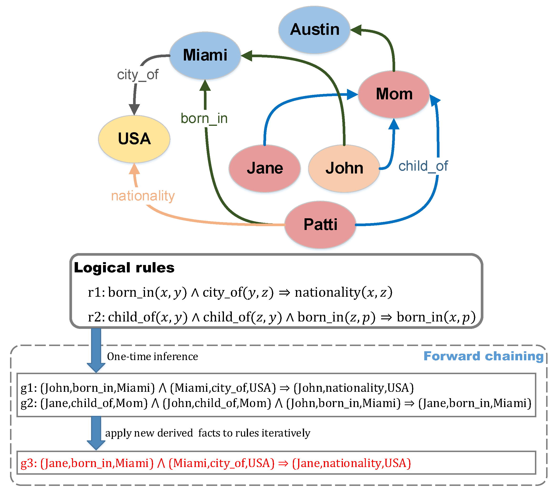
On the other hand, generating all groundings of one rule is costly, since the number of candidate entities is usually very large. Nevertheless, many groundings are meaningless and unnecessary, for example, given a logical rule $\forall x,y,(x,\mathrm{child}\_\mathrm{of},y)\Rightarrow (y,\mathrm{parent}\_\mathrm{of},x)$, groundings like $(\mathrm{USA},\mathrm{child}\_\mathrm{of},\mathrm{Mom})\Rightarrow (\mathrm{Mom},\mathrm{parent}\_\mathrm{of},\mathrm{USA})$ are useless. Therefore, most of the existing methods perform one time logical inference over logical rules and observed KG facts to generate valid groundings for modeling rules. However, they ignore forward chaining inference, which can further apply new derived facts to rules iteratively to generate more valid groundings. As far as we are concerned, the logical rules can be modeled more accurately with more valid groundings. As shown in Figure 1, given a toy KG at the top and two rules r1,r2  in the middle, we can only generate groundings g1 and g2 after applying the facts of KG to these rules via one time inference, as previous works did. However, according to forward chaining, we can further generate g3 by applying a new fact (Jane,born_in,Miami) to rule r1.

Based on these observations, this paper proposes Soft Logical Rules enhanced Embedding (SoLE), a novel paradigm of KG embedding enhanced with a joint training algorithm over soft rules and KG facts, as well as forward chaining inference over logical rules. Specifically, SoLE contains two stages: grounding generation and embedding learning. In the first stage, we extract soft rules with certain confidences via a modern rule mining system and then use the rule engine to perform forward chaining over these soft rules and KG facts to generate more groundings. At the stage of embedding learning, we devise a joint training algorithm that learns KG embeddings using both KG facts and soft rules simultaneously. Here, facts are modeled by the existing KG embedding method, groundings are modeled by t-norm fuzzy logics, and soft rules are modeled by their corresponding groundings. The confidence of one soft rule is treated as the probability this rule holds. Then, the Mean Squared Error (MSE) between the confidences of soft rules and the likelihood of these rules determined by their groundings is used to estimate these rules. In this way, the facts in groundings can capture the logical background knowledge of soft rules so as to learn better embeddings. Finally, the algorithm learns the embeddings by summing up to minimizing a global loss over both the loss function for KG facts and the L2 loss for soft rules.

We empirically evaluated SoLE with the link prediction task on two large scale public KGs, Freebase and DBpedia. Experimental results indicated that: (i) SoLE significantly and consistently outperformed the basic embedding models and the state-of-the-art models with soft rules; (ii) compared to the work RUGE [14], our joint training algorithm achieved significantly better performance; and (iii) compared to one time inference, forward chaining indeed helped to learn more predictive embeddings.

Our main contributions are summarized as follows:

• We devise a novel joint training algorithm that learns KG embeddings using both KG facts and soft rules simultaneously. Through this joint training, the background knowledge of soft rules can be directly injected into embeddings.
• We introduce forward chaining inference to KG embedding model with logical rules, so as to generate more valid groundings for better modeling rules. As far as we know, this is the first attempt to use forward chaining for generating groundings.
• We present an empirical evaluation that demonstrates the benefits of our joint algorithm and forward chaining.

The remainder of this paper is organized as follows. We first give some preliminaries about our work in Section 2 and review the related works in Section 3. Then, we detail our approach in Section 4. After that, experiments and results are reported in Section 5. Finally, we conclude our work in Section 6.

2. Preliminaries

In this section, we introduce two necessary preliminaries, i.e., knowledge graph embedding and forward chaining, for readers to follow the rest of the paper.

2.1. Knowledge Graph Embedding

A KG $\mathcal{K}=\{\mathcal{E},\mathcal{R},\mathcal{T}\}$ contains a set of entities $\mathcal{E}$, a set of relations $\mathcal{R}$, and a set of triples or facts $\mathcal{T}=\left\{\right(h,r,t\left)\right|h,t\in \mathcal{E};r\in \mathcal{R}\}\subseteq \mathcal{E}\times \mathcal{R}\times \mathcal{E}$. The symbols h, r, and t denote head entity, relation, and tail entity, respectively, in a triple $(h,r,t)$. An example of such a triple can be (Paris, isCapitalOf, France).

KG embedding aims to embed all entities and relations into a low-dimensional continuous vector space, usually as vectors or matrices called embeddings. A typical KG embedding technique consists of three steps as follows. First, the assumptions of the entities and relations vector space should be given. Entities are usually represented as vectors, i.e., deterministic points in the vector space, and relations are typically taken as operations in the vector space, which can be represented as vectors, matrices, or tensors. Then, a score function $f:\mathcal{E}\times \mathcal{R}\times \mathcal{E}\to \mathbb{R}$ will be defined based on these assumptions to measure the plausibility of each fact in KG. Facts observed in the KG tend to have larger scores than those that have not been observed. Finally, embeddings can be obtained by maximizing the total plausibility of all facts measured by the score function.

Based on the different design of score functions, the KG embedding techniques can be categorized into three types: translation based models, linear models, and neural network based models. We now briefly describe these types and introduce a commonly used model for each type. The readers can see [15,16] for a thorough review.

2.1.1. Translation Based Models

Translation based models assume entities and relations are both represented as vectors. They  measure the plausibility of a fact as the distance between two entities, usually after a translation carried out by the relation. For a true triple, after being translated by the relation, the head entity is close to the tail entity in the embeddings’ vector space.

TransE: TransE [17] is the most representative translation based model. Entities and relations are represented as vectors in space ${\mathbb{R}}^d$. For a triple $(h,r,t)$, $\mathbf{h}$, $\mathbf{t}$, and $\mathbf{r}$ are denoted as vectors of entities $h,t$ and relation r respectively. The score function of TransE is then defined as the negative distance between $\mathbf{h}+\mathbf{r}$ and $\mathbf{t}$, i.e.,

$$f(h,r,t)={-\parallel \mathbf{h}+\mathbf{r}-\mathbf{t}\parallel }_{1/2}.$$

(1)

The score of $(h,r,t)$ is expected to be large if it holds. The training process of TransE is to minimize a pairwise ranking loss function as follows:

$$\sum _{(h,r,t)\in \mathcal{T}}\sum _{(h^{\prime },r^{\prime },t^{\prime })\in {\mathcal{T}}^{\prime }}max(0,\gamma -f(h,r,t)+f(h^{\prime },r^{\prime },t^{\prime })),$$

$$\begin{array}{c}\hfill {\mathcal{T}}^{\prime }=\left\{(h^{\prime },r,t)\right|h^{\prime }\in \mathcal{E}\wedge h^{\prime }\ne h\wedge (h,r,t)\in \mathcal{T}\}\\ \hfill \cup \left\{(h,r,t^{\prime })\right|t^{\prime }\in \mathcal{E}\wedge t^{\prime }\ne t\wedge (h,r,t)\in \mathcal{T}\},\end{array}$$

(2)

where ${\mathcal{T}}^{\prime }$ is a set of sampled negative examples and $\gamma >0$ is a margin hyperparameter separating positive examples from negative ones. Here, the observed triples in $\mathcal{T}$ are treated as positive examples, and the negative ones are generated by corrupting either the head entity or the tail entity of observed triples with the random entities sampled uniformly from $\mathcal{E}$.

2.1.2. Linear Models

Linear models assume that entities are represented as vectors and relations as matrices. They  measure the plausibility of a fact as the similarity between two entities, usually after a linear mapping operation via the relation. In this case, for a true triple, the head entity can be linearly mapped, by the relation matrix, to somewhere close to the tail entity in the embeddings’ vector space.

ComplEx: ComplEx [18] is the most commonly used linear model. Entities and relations are represented as vectors in complex space ${\mathbb{C}}^d$. Given any triple $(h,r,t)$, a multi-linear dot product is used to score the triple. Thus, the score function is defined as follows:

$$f(h,r,t)=\mathrm{Re}\left({\mathbf{h}}^{\top }\mathrm{diag}\left(\mathbf{r}\right)\overline{\mathbf{t}}\right)=\mathrm{Re}(\sum _{i=0}^{d-1}{\left[\mathbf{r}\right]}_i·{\left[\mathbf{h}\right]}_i·{\left[\overline{\mathbf{t}}\right]}_i),$$

(3)

where the $\mathrm{Re}(·)$ function takes the real part of a complex value and the $\mathrm{diag}(·)$ function constructs a diagonal matrix from $\mathbf{r}$; $\overline{\mathbf{t}}$ is the conjugate of $\mathbf{t}$; ${[·]}_i$ is the $i^{\mathrm{th}}$ entry of a vector. The higher the score, the more likely the triple holds. For the prediction of triples, ComplEx further devises a function $\varphi :\mathcal{E}\times \mathcal{R}\times \mathcal{E}\to (0,1)$, which maps the score $f(h,r,t)$ to a continuous truth value from the range of $(0,1)$, i.e.,

$$\varphi (h,r,t)=\sigma \left(f(h,r,t)\right)=\sigma \left(\mathrm{Re}\left({\mathbf{h}}^{\top }\mathrm{diag}\left(\mathbf{r}\right)\overline{\mathbf{t}}\right)\right),$$

(4)

where the $\sigma (·)$ function denotes the sigmoid function. ComplEx learns the entity and relation embeddings by minimizing the logistic loss function, i.e.,

$$\sum _{(h,r,t)\in \mathcal{T}\cup {\mathcal{T}}^{\prime }}log(1+exp(-y_{hrt}·f(h,r,t))),$$

(5)

where $y_{hrt}=\pm 1$ is the label of a positive or negative triple $(h,r,t)$ and ${\mathcal{T}}^{\prime }$ is the same one defined in Equation (2).

2.1.3. Neural Network Based Models

Neural network based models assume that entities and relations are represented as vectors. They exploit a multi-layer neural network with nonlinear features to measure the plausibility of facts. For a triple $(h,r,t)$, neural network models take its vector representations $\mathbf{h}$, $\mathbf{t}$, and $\mathbf{r}$ as input and then output the probability of the triple to be true after the feed-forward process.

ConvE: ConvE [19] is a neural network based model where the latent semantics of input entities and relations are modeled by convolutional and fully connected layers. Entities and relations are represented as vectors in space ${\mathbb{R}}^d$. The score function is defined as follows:

$$f(h,r,t)=g(\mathrm{vec}(g(\mathrm{concat}(\widehat{\mathbf{h}},\widehat{\mathbf{r}})*\omega ))\mathbf{W})\mathbf{t},$$

(6)

where $\widehat{\mathbf{h}}$ and $\widehat{\mathbf{r}}$ denote a 2D reshaping of $\mathbf{h}$ and $\mathbf{r}$, respectively; the $\mathrm{concat}(·)$ function concatenates two matrices $\widehat{\mathbf{h}}$ and $\widehat{\mathbf{r}}$; $\omega$ denotes a set of filters; * denotes a convolution operator; the $\mathrm{vec}(·)$ function reshapes the tensor produced by the convolution layer into a vector; $g(·)$ denotes a nonlinear function. ConvE applies the sigmoid function $\sigma (·)$ as the last layer activation to the score, which is $p_{hrt}=\sigma \left(f(h,r,t)\right)$, and learns the embeddings by minimizing the following binary cross-entropy loss function:

$$\sum _{(h,r,t)\in \mathcal{T}\cup {\mathcal{T}}^{\prime }}-(y_{hrt}·log\left(p_{hrt}\right)+(1-y_{hrt})·log(1-p_{hrt})),$$

(7)

where the definitions of $\mathcal{T},{\mathcal{T}}^{\prime }$, and $y_{hrt}$ are the same as the above Equation (5).

2.2. Logical Rule and Forward Chaining

In this paper, we refer to a logical rule as a Horn clause (a subset statements of first order logic) rule, represented in the form of an implication $p_1\wedge p_2\wedge \cdots \wedge p_n\Rightarrow q$, where $p_i(i=1,\cdots ,n)$ and q are positive atoms. The left side of the implication “⇒” is known as the premise, i.e., a conjunction of several atoms, and the right side the conclusion, which contains a single atom. Given a KG $\mathcal{K}=\{\mathcal{E},\mathcal{R},\mathcal{T}\}$, an atom can be $(x,\mathrm{city}\_\mathrm{of},y)$, where $x,y$ are variables from $\mathcal{E}$ and “$\mathrm{city}\_\mathrm{of}$” is a concrete relation. An example of a logical rule over $\mathcal{K}$ can be:

$$\forall x,y:(x,\mathrm{child}\_\mathrm{of},y)\Rightarrow (y,\mathrm{parent}\_\mathrm{of},x),$$

(8)

which means that if two entities are linked by relation “$\mathrm{child}\_\mathrm{of}$”, then they should also be linked by relation “$\mathrm{parent}\_\mathrm{of}$”.

When we propositionalize a logical rule by instantiating all variables in the rule with concrete entities in $\mathcal{E}$, we get a grounding of the rule (or a ground rule). For instance, one grounding of the above example rule can be: $(\mathrm{Jane},\mathrm{child}\_\mathrm{of},\mathrm{Mom})\Rightarrow (\mathrm{Mom},\mathrm{parent}\_\mathrm{of},\mathrm{Jane})$. Apparently, propositionalizing rules to get all groundings is costly, since the entity vocabulary $\mathcal{E}$ is large. Nevertheless, many groundings are meaningless and unnecessary, such as $(\mathrm{USA},\mathrm{child}\_\mathrm{of},\mathrm{Mom})\Rightarrow (\mathrm{Mom},\mathrm{parent}\_\mathrm{of},\mathrm{USA})$. Therefore, in practice, we take as valid groundings only those whose premise triples are observed in or derived from $\mathcal{K}$, while the conclusion triples are not observed in $\mathcal{K}$.

The key role of logical rules is that we can perform reasoning through them over a given KG to derive new facts. The process of reasoning starts from the premises of a rule to reach a certain conclusion. That means if some facts in KG are the instances of the premises in a rule, the conclusion instance then can be derived. There are several methods to perform the reasoning. Forward chaining is one of the main methods, which typically works in the way of three phase cycles, also named the match-select-act cycle. More precisely, in one cycle, forward chaining firstly matches the current observed or derived facts in KG against the premises of all known rules to find out the satisfied rules. Then, it selects one rule via some strategies from these satisfied rules. Lastly, it derives the conclusion of the selected rule and puts it into KG as a new fact if it is not in KG. The cycle is repeated until no more new facts are derived.

Notably, during the process of forward chaining, when we derive a new fact from a rule, we also get its grounding, whose conclusion is this new fact. Therefore, we can obtain plenty of corresponding groundings of rules after performing forward chaining inference.

3. Related Work

Recent years have witnessed growing interest in developing KG embedding models. Most of the existing works learn embeddings based solely on the observed triples in KG, which suffer from the problem of data sparsity. To alleviate such a problem and learn better embeddings, many researchers tried to utilize extra useful information, such as textual descriptions, entity types, relation paths, and first order logic rules.

Since rules introduce rich background information and are useful for knowledge acquisition and inference, combining KG embedding with logical rules becomes a focus of current research. There are two kinds of logical rules employed by previous works, i.e., hard rules, which are manually created or validated, and soft rules, which are extracted from knowledge graphs themselves. As for hand rules, Wang et al. [20] first devised a framework using logical rules as constraints to refine the embedding model, and Wei et al. [21] attempted to combine rules and the embedding model via Markov logic networks. In their works, rules were modeled separately from the embedding model, employed as post-processing steps, and thus, failed to learn more predictive embeddings. Subsequently, Rocktaschel et al. [22] and Guo et al. [23] proposed joint models, which embedded KG facts and ground rules simultaneously. Although their works also learned embeddings jointly, they were not able to support the uncertainty of soft rules. In addition, Demeester et al. [24] imposed a partial ordering on relation embeddings through implication rules to avoid the costly propositionalization, and Minervini et al. [25] utilized rules to regularize the embedding model via adversarial sets.

As for soft rules, Minervini et al. [12] considered the soft equivalence and inversion rules to regularize embeddings. Ding et al. [13] added a non-negativity constraint on entity embeddings and approximate entailment constraint on relation embeddings with soft rules. Guo et al. [14] proposed RUGE and considered employing soft rules. This enabled an embedding model to learn simultaneously from KG triples, derived triples in an iterative manner, where each iteration alternated between a soft label prediction stage, that was to predict soft labels for derived triples by groundings and currently learned embeddings, and an embedding rectification stage, that was to update current embeddings by KG triples and derived triples. All these methods either cannot support the transitivity and composition rules or are incapable of encoding the correlation of facts contained in soft rules, while our method injects such background knowledge of rules into KG embeddings by jointly training soft rules and KG triples. Furthermore, a recent work [26] conducted rule learning and embedding learning iteratively to explore the mutual benefits between them so that the learned soft rules could improve embedding quality. Qu et al. [27] modeled logical rules via the Markov logic network and inferred the unobserved triples (i.e., hidden variables) to improve KG embeddings. In contrast to them, our method enhanced KG embeddings through directly injecting the background knowledge of soft rules, which was much easier to conduct.

4. Our Method

This section presents our method SoLE. We first give an overview of our method. Then, we detail the two stages of SoLE, grounding generation, and embedding learning respectively. Finally, we analyze the time and space complexity of our method and discuss its flexibility.

4.1. Overview

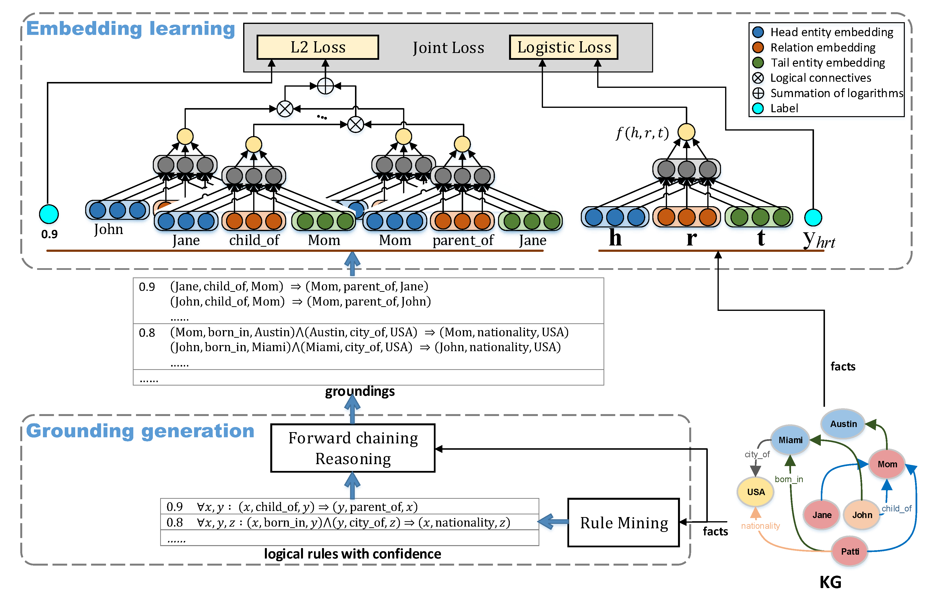
Here, we give the overview of our method SoLE based on a commonly used embedding model ComplEx, which was mentioned in Section 2.1. SoLE contains two stages, grounding generation and embedding learning. In the grounding generation stage, there are two modules, rule mining and forward chaining reasoning. The rule mining module takes the KG triples and the configuration for extracting rules, such as the confidence threshold of rules and the maximum length of rules, as inputs. Then, it will automatically extract soft rules based on these inputs. After that, the extracted soft rules, together with the KG triples, will be sent to the forward chaining reasoning module, where it performs forward chaining over soft rules and triples to infer groundings. Finally, the groundings will be output to the embedding learning stage.

In the embedding learning stage, followed by ComplEx, KG triples are modeled as the similarity of the head and tail entity after a linear mapping operation via the relation and scored by the function $f(h,r,t)$ (defined in Equation (3)). The truth value of KG triples are determined by the the function $\varphi (h,r,t)$ (defined in Equation (4)), indicating how likely a triple holds. As for a logical rule, it is modeled as the conjunction of all its groundings. A grounding is modeled by the product t-norm and expressed as logic formulae, constructed by combining atoms with logical connectives (e.g., ∧ and ⇒). Thus, the truth value of a grounding can be determined by the truth values of its component triples via specific logical connectives. Subsequently, the truth value of one logical rule can be defined by multiplying the truth values of its groundings. In practice, for the sake of convenience, the truth value of one rule is measured by the summation of the logarithms of the truth values of its groundings instead of the product. Finally, SoLE minimizes a joint loss over the KG triples and soft logical rules, where the logistic loss (defined in Equation (5)) is optimized for the triples and the L2 loss for the rules, to learn entity and relation embeddings compatible with both triples and rules. Moreover, the training procedure of this stage is under the Open World Assumption (OWA), which states that KGs contain only true triples, and non-observed triples can be either false or just missing. Negative samples are generated by the local closed world assumption, which assumes triples not contained in KG are false.

Figure 2 illustrates the overall procedure of SoLE given a toy KG example. As shown in Figure 2, in the grounding generation stage, soft rules like Rule (8) with confidence value $0.9$ will be extracted from the rule mining module. According to the extracted soft rules, the forwarding chaining reasoning module will output the groundings of rules, such as $(\mathrm{Jane},\mathrm{child}\_\mathrm{of},\mathrm{Mom})\Rightarrow (\mathrm{Mom},\mathrm{parent}\_\mathrm{of},\mathrm{Jane})$. These groundings and the given KG triples are input as training data into the embedding learning stage to learn jointly the KG embeddings. In what follows, we will describe these two stages of SoLE in detail.

4.2. Grounding Generation

The grounding generation stage consists of the rule mining module, which extracts soft rules, and the forward chaining reasoning module, which infers groundings from these rules. We detail these two modules as follows.

4.2.1. Rule Mining

In this module, we employ the state-of-the-art rule mining system, AMIE+ [28], to mine Horn rules from the KG triples. AMIE+ provides two kinds of confidence to measure how likely a rule holds, i.e., the standard confidence and the PCA (the PCA (Partial Completeness Assumption) assumes that if we know one y for a given conclusion triple $(x,\mathrm{r},y)$ of one rule, then we know all y for that x and $\mathrm{r}$.) confidence. We use the PCA confidence since its partial completeness assumption is more permissive. Moreover, there are various types of restrictions defined in AMIE+ to help mine the desirable rules. For example, the PCA confidence threshold restricts the PCA confidence of output rules whose value must not be less than the threshold, and the maximum rule length restricts the length of output rules, where the length of a rule means the number of atoms in the premises of the rule. After receiving the KG triples and the configuration of these restrictions, the rule mining module will execute the AMIE+ algorithm and output all the matching rules with their PCA confidence values.

4.2.2. Forward Chaining Reasoning

In this module, we use the rule engine system Drools [29] to perform forward chaining efficiently. Specifically, the main process of the forward chaining reasoning module follows the steps below.

• Convert the rule format: Rules extracted from rule mining module can not be used directly by Drools. Drools supports only the rules defined by its own syntax; therefore, we need to parse the extracted rules into the Drools rule format one by one. While converting the original Horn rule into the Drools rule, we add the condition in the Drool rule to ensure that the derived triples are inserted into working memory (place that holds a set of triples) only once in the case of loop inference. Listing 1 shows the data structure defined for groundings and Listing 2 demonstrates a Drools rule converted from a Horn rule $\forall a,b:(b,/\mathrm{music}/\mathrm{instrument}/\mathrm{variation},a)\Rightarrow (a,/\mathrm{music}/\mathrm{instrument}/\mathrm{family},b)$ with its PCA confidence value equal to 0.9.
• Perform forward chaining: After converting the rule format, we map the extracted Horn rules to the Drools rules. Then, we use the Drools’ API to perform reasoning over these rules and the KG triples. Equipped with the Rete algorithm [30], a fast pattern matching algorithm, Drools can achieve forward chaining efficiently. Finally, the forward chaining reasoning module will output all the derived groundings associated with the rules they belong to after finishing the inference. As mentioned in Section 2.2, we only infer valid groundings from observed and derived triples.

Listing 1. Data structure of groundings.

Listing 1. Data structure of groundings.

Listing 2. Drools rule example.

Listing 2. Drools rule example.

4.3. Embedding Learning

This section introduces a joint training algorithm, which enables an embedding model to learn simultaneously from KG triples and soft rules. In what follows, we first describe our learning resources, and then discuss how to model them in the context of KG embeddings. At last, we give our training objective and detail how to learn embeddings from it.

4.3.1. Learning Resources

Given a KG $\mathcal{K}=\{\mathcal{E},\mathcal{R},\mathcal{T}\}$ with a set of triples $\mathcal{T}=\left\{(e_i,r_k,e_j)\right\}$, where head entity $e_i$, tail entity $e_j\in \mathcal{E}$, and relation $r_k\in \mathcal{R}$. We obtain our learning resources as follows.

Labeled triples: As we have mentioned in Section 2.1, we take the observed triples in $\mathcal{T}$ as positive examples. For each positive triple $(e_i,r_k,e_j)$, we generate negative triple $(e_i^{\prime },r_k,e_j)$ or $(e_i,r_k,e_j^{\prime })$ by randomly corrupting the head entity $e_i$ or the tail entity $e_j$, where $e_i^{\prime }\in \mathcal{E}\backslash \left\{e_i\right\}$ and $e_j^{\prime }\in \mathcal{E}\backslash \left\{e_j\right\}$. Then, we assign a label $y_l$ to each triple $x_l$, $y_l=1$ if $x_l$ is positive and $y_l=-1$ otherwise. A labeled triple is denoted as $(x_l,y_l)$. Let $\mathcal{L}=\left\{(x_l,y_l)\right\}$ represent the set of these labeled triples.

Soft rules. We denote a set of Horn clause rules extracted from the rule mining module as $\mathcal{F}={\left\{(f_p,c_p)\right\}}_{p=1}^P$, where $f_p$ is the $p^{\mathrm{th}}$ logical rule defined over $\mathcal{K}$, $c_p\in (0,1]$ is the confidence value of $f_p$, and P is the number of all soft rules. For each logical rule $f_p$, we denote its groundings generated by the grounding generation stage as ${\mathcal{G}}_p={\left\{g_{pq}\right\}}_{q=1}^{Q_p}$, where $Q_p$ is the number of groundings and $g_{pq}$ is the $q^{\mathrm{th}}$ grounding in ${\mathcal{G}}_p$, e.g., $(e_u,r_m,e_v)\Rightarrow (e_v,r_n,e_u)$ given the form of $f_p$ as $\forall x,y:(x,r_m,y)\Rightarrow (y,r_n,x)$. Let $\mathcal{G}={\cup }_{p=1}^P{\mathcal{G}}_p$ denote the set of all these groundings.

4.3.2. Triple and Rule Modeling

To model triples, based on the score function of the existing KG embedding model, we aim to find a mapping function $\varphi :\mathcal{E}\times \mathcal{R}\times \mathcal{E}\to (0,1)$, so as to map the score of one triple $(e_i,r_k,e_j)$ to a continuous truth value lying in the range of $(0,1)$. Such a soft truth value indicates the probability that the triple holds. In our method SoLE, we followed ComplEx and used function $f(·)$ (defined in Equation (3)) as the score function, as well as function $\varphi (·)$ (defined in Equation (4)) as the mapping function. That is to say, given a triple $(e_i,r_k,e_j)$, its truth value is measured by $\varphi (e_i,r_k,e_j)=\sigma (\mathrm{Re}({\sum }_{s=0}^{d-1}{\left[{\mathbf{r}}_{\mathbf{k}}\right]}_s·{\left[{\mathbf{e}}_{\mathbf{i}}\right]}_s·{\left[\overline{{\mathbf{e}}_{\mathbf{j}}}\right]}_s))$.

To model groundings, we used the product t-norm, which belongs to t-norm fuzzy logic [31], and defined the truth value of a grounding as a composition of the truth values of its component triples through specific logic connectives. We assumed that the probabilities of the triples in a grounding were independent conditioned on embeddings. Then, according to the product t-norm, the compositions related to logical conjunction and negation can be defined as follows:

$$\begin{array}{cc}\hfill & \pi (a\wedge b)=\pi \left(a\right)·\pi \left(b\right),\hfill \\ \hfill & \pi (\neg a)=1-\pi \left(a\right),\hfill \end{array}$$

(9)

where a and b are two logic formulas, which can be either a single triple (atom) or the compositions of triples through logic connectives; and $\pi \left(a\right)$ is the truth value of a, which indicates to what degree the formulae are true. If a is a single triple, such as $(e_i,r_k,e_j)$, we can obtain $\pi \left(a\right)=\varphi (e_i,r_k,e_j)$. Given these compositions, we can compute the truth value of any complex formulae recursively, e.g.,

$$\begin{array}{cc}\hfill & \pi (a\vee b)=\pi \left(a\right)+\pi \left(b\right)-\pi \left(a\right)·\pi \left(b\right),\hfill \\ \hfill & \pi (a\Rightarrow b)=\pi (\neg a\vee b)=\pi \left(a\right)·\left(\pi \right(b)-1)+1,\hfill \\ \hfill & \pi (a\wedge b\Rightarrow c)=\pi \left(a\right)·\pi \left(b\right)·\left(\pi \right(c)-1)+1.\hfill \end{array}$$

(10)

For instance, given a grounding $g_{pq}\triangleq (e_u,r_m,e_v)\Rightarrow (e_v,r_n,e_u)$, its truth value is calculated as $\pi \left(g_{pq}\right)=\varphi (e_u,r_m,e_v)·(\varphi (e_v,r_n,e_u)-1)+1$.

To model logical rules, we followed [22] and embedded first order logic through explicit groundings. For rules with universal quantification like $f_p$, we computed its truth value as:

$$\pi \left(f_p\right)=\pi \left({\wedge }_{q=1}^{Q_p^{\prime }}{g}_{pq}\right),$$

(11)

where $Q_p^{\prime }$ is the number of all the $f_p$’s groundings propositionalized from the set $\mathcal{E}\times \mathcal{E}$. Again, we assumed that the groundings in $Q_p^{\prime }$ were independent. Besides, as we mentioned in Section 2.2, it is non-trivial to get all groundings, and many groundings are unnecessary. Thus, we used valid groundings $Q_p$ of $f_p$ to calculate its truth value and assumed that $Q_p^{\prime }$ equaled $Q_p$. Finally, we can simplify Equation (11) to:

$$\pi \left(f_p\right)=\prod _{q=1}^{Q_p}\pi \left(g_{pq}\right).$$

(12)

If some groundings are not independent, we can think of this equation as an approximation.

4.3.3. Training Objective

Given a set of labeled triples $\mathcal{L}=\left\{(x_l,y_l)\right\}$ and a set of soft rules $\mathcal{F}={\left\{(f_p,c_p)\right\}}_{p=1}^P$ with a set of their groundings $\mathcal{G}={\cup }_{p=1}^P{\mathcal{G}}_p$, we would like to learn the relation and entity embeddings $\mathsf{\Theta }\in {\mathbb{C}}^d$ from them.

To this end, we minimize a global loss over $\mathcal{L}$ and $\mathcal{F}$, so as to find embeddings that could predict the labels of triples contained in $\mathcal{L}$, while imitating the confidences of rules in $\mathcal{F}$. The training objective was:

$$\underset{\mathsf{\Theta }}{min}\frac{1}{\left|\mathcal{L}\right|}\sum _{(x_l,y_l)\in \mathcal{L}}L(-f\left(x_l\right)·y_l)+\frac{1}{\left|\mathcal{F}\right|}\sum _{(f_p,c_p)\in \mathcal{F}}{\parallel \pi \left(f_p\right)-c_p\parallel }^2,$$

(13)

where $f(·)$ is the score function w.r.t. $\mathsf{\Theta }$; $L\left(x\right)=log(1+exp(x\left)\right)$ is the soft-plus function; and $\pi \left(f_p\right)$ is defined in Equation (12) w.r.t. $\mathsf{\Theta }$. We further imposed $l_2$ regularization on $\mathsf{\Theta }$ to avoid overfitting. The former logistic loss of Equation (13) enforces that positive triples have truth values close to one, while negative ones close to −1. Meanwhile, the latter L2 loss enforces that the truth values of rules stay close to their confidences. Gradient descent algorithms can be used to solve this optimization problem. However, it is difficult to compute the gradients of $\pi \left(f_p\right)$ in the latter L2 loss, since it contains many multiply operations. To overcome this difficulty, we replaced the product of $\pi \left(f_p\right)$ with the summation of the logarithms, i.e., the squared error $\parallel \pi \left(f_p\right)-c_p{\parallel }^2$ changes to $\parallel log\pi \left(f_p\right)-log{c}_p{\parallel }^2$. Here, $log\pi \left(f_p\right)$ equals ${\sum }_{q=1}^{Q_p}log\pi \left(g_{pq}\right)$ according to Equation (12). Thus, the training objective can be rewritten as:

$$\begin{array}{cc}\hfill \underset{\mathsf{\Theta }}{min}& \left(\frac{1}{\left|\mathcal{L}\right|}\sum _{(x_l,y_l)\in \mathcal{L}}L(-f\left(x_l\right)·y_l)+\frac{1}{\left|\mathcal{F}\right|}\sum _{(f_p,c_p)\in \mathcal{F}}{\parallel \sum _{q=1}^{Q_p}log\pi \left(g_{pq}\right)-log{c}_p\parallel }^2\right).\hfill \end{array}$$

(14)

The embedding learning procedure of our method is shown in Algorithm 1. We took the given KG triples $\mathcal{T}$ and extracted soft rules $\mathcal{F}$ with their groundings $\mathcal{G}$ from the first stage as inputs. Then, we carried out the optimization and learned the embeddings through N iterations. At each iteration, we first sampled a mini-batch ${\mathcal{T}}^b$ and ${\mathcal{G}}^b$ from $\mathcal{T}$ and $\mathcal{G}$. After that, a set of negatives ${\mathcal{T}}_{neg}^b$ was generated by corrupting the triples in ${\mathcal{T}}^b$. Next, we assigned the label one or −1 for each triple in ${\mathcal{T}}_{neg}^b\cup {\mathcal{T}}^b$ and constructed the set of labeled triples ${\mathcal{L}}^b$ (Lines 6–8). Then, we partitioned the batch groundings ${\mathcal{G}}^b$ into ${\cup }_{p=1}^{P^{\prime }}{\mathcal{G}}_p^b$ by their associated rules contained in $\mathcal{F}$. According to ${\cup }_{p=1}^{P^{\prime }}{\mathcal{G}}_p^b$, we obtained a batch of rules ${\mathcal{F}}^b={\left\{(f_p,c_p)\right\}}_{p=1}^{P^{\prime }}$ (Line 10). Finally, we conducted gradient descent on these mini-batches and updated the embeddings. In practice, we used Stochastic Gradient Descent (SGD) in mini-batch mode as our optimizer, with Adam [32] to tune the learning rate. Embeddings learned in this way are required to be compatible with not only triples, but also soft rules.

4.4. Discussions

4.4.1. Complexity

In the embedding learning stage of SoLE, we followed ComplEx to represent entities and relations as complex valued vectors. Thus, the space complexity was $O(n_{e}d+n_{r}d)$, where d is the dimensionality of the embedding space, $n_e=\left|E\right|$ is the number of entities, and $n_r=\left|R\right|$ is the number of relations. As we can see from Algorithm 1, during the learning procedure, each iteration required a time complexity of $O(n_{l}d+n_g(M+1)d)$, where $n_l=\left|L^b\right|$ is the number of labeled triples in a mini-batch, $n_g=\left|G^b\right|$ is the number of groundings in a mini-batch, and M is the maximum rule length. SoLE had a space and time complexity that scaled linearly with d, which was the same as ComplEx. However, the time complexity of SoLE was much larger than ComplEx, which only required $O\left(n_{l}d\right)$ per iteration, since SoLE needed to compute the truth values of rules besides the scores of triples. In addition, the space and time complexity of the grounding generation stage were trivial compared to the embedding learning stage, due to the high efficiency of reasoning and the restrictions on the rule mining module in practice, e.g., the PCA confidence threshold not lower than 0.5 and the length of rules not longer than two. Therefore, we could ignore it when analyzing the time and space complexity of SoLE.

Algorithm 1 Joint training algorithm of SoLE.

Require:     KG triples $\mathcal{T}=\left\{(e_i,r_k,e_j)\right\}$;     Logical rules $\mathcal{F}=\left\{(f_p,c_p)\right\}$ and their corresponding groundings $\mathcal{G}={\cup }_{p=1}^P{\mathcal{G}}_p$. Ensure:     Entity and relation embeddings $\mathsf{\Theta }$. 1: Initialize entity and relation embeddings ${\mathsf{\Theta }}^{\left(0\right)}$ randomly 2: for$n\leftarrow 1\mathrm{to}N$do                     ▹N is the number of iterations 3:    Sample a mini-batch ${\mathcal{T}}^b$,${\mathcal{G}}^b$ from $\mathcal{T}$,$\mathcal{G}$ 4:    Generate a set of negative triples ${\mathcal{T}}_{neg}^b$ from ${\mathcal{T}}^b$ 5:    ${\mathcal{L}}^b\leftarrow \varnothing$                        ▹${\mathcal{L}}^b$ is the set of labeled triples 6:    for each $x_l\in {\mathcal{T}}_{neg}^b\cup {\mathcal{T}}^b$ do 7:       $y_l=\pm 1$ 8:       ${\mathcal{L}}^b\leftarrow {\mathcal{L}}^b\cup \left\{(x_l,y_l)\right\}$ 9:    end for 10:    Generate a batch of logical rules ${\mathcal{F}}^b$ from ${\mathcal{G}}^b$ and $\mathcal{F}$ 11:    ${\mathsf{\Theta }}^{\left(n\right)}\leftarrow {\mathsf{\Theta }}^{(n-1)}-\eta \left(\frac{1}{|{\mathcal{L}}^b|}{\sum }_{(x_l,y_l)\in {\mathcal{L}}^b}{\nabla }_{\mathsf{\Theta }}L(-f\left(x_l\right)·y_l)+\frac{1}{|{\mathcal{F}}^b|}{\sum }_{(f_p,c_p)\in {\mathcal{F}}^b}{\nabla }_{\mathsf{\Theta }}{\parallel {\sum }_{g_{pq}}log\pi \left(g_{pq}\right)-log{c}_p\parallel }^2\right)$                             ▹cf. Equation (14) 12: end for 13: return${\mathsf{\Theta }}^{\left(N\right)}$

4.4.2. Flexibility

Just like RUGE, our method was generic and flexible from the following two aspects. On the one hand, in addition to ComplEx, SoLE could enhance a variety of embedding models through integrating soft rules into them, as long as a mapping function is properly designed for modeling rules, like the one defined in Equation (4). On the other hand, in addition to the product t-norm, we could use other types of t-norm based fuzzy logics, e.g., the Łukasiewicz t-norm and the minimum t-norm, to define the logical compositions in Equations (9)–(12).

5. Experiment

When conducting experiments on SoLE, we wanted to explore the following two questions:

• Whether the devised joint training algorithm and the introduction of forward chaining of SoLE really provided benefits for embeddings compared to the state-of-the-art KG embedding models with soft rules: To test this, we evaluated the performance of SoLE on the link prediction task, which has been widely applied in previous KG embedding works.
• Considering the groundings generated by forward chaining, whether they were more helpful for embeddings than those generated by one time inference and to what degree if this is true: To do this, we compared the effect of forward chaining and one time inference on the link prediction task and analyzed the results.

Besides, we will discuss the influence of the PCA confidence threshold on our method, the convergence of the training process in SoLE, and the whole runtime of SoLE. Notably, we used the TensorFlow framework (GPU) along with Python 3.6 to conduct our experiments. All experiments were executed on a Linux server with processor Intel(R) Xeon(R) Gold 5118 CPU @ 2.30 GHz, 128 GB RAM, and an NVIDIA GeForce GTX 1080 GPU.

5.1. Evaluation Task

We evaluated our method on the link prediction task. This task aimed to complete a triple $(e_i,r_k,e_j)$ with the head entity $e_i$ or tail entity $e_j$ missing, which meant to predict $e_i$ given $(r_k,e_j)$ or $e_j$ given $(e_i,r_k)$, i.e., to answer a query $(?,r_k,e_j)$ or $(e_i,r_k,?)$.

5.2. Experimental Setup

5.2.1. Datasets and Configuration

Two datasets were used in our experiments, including FB15Kand DB100K. FB15K, first released by Bordes et al. [17], is a subset of a large collaborative knowledge base Freebase, while DB100K, created by Guo et al. [14], was generated from the large knowledge graph DBpedia. For both datasets, triples were split into training, validation, and test sets, which were used for embeddings’ learning, hyper-parameter tuning, and evaluation, respectively. The detailed statistics of the datasets are shown in

Table 1. Statistics of the datasets, where the columns denote the number of entities, relations, training/validation/test triples, extracted rules, and their groundings, respectively.

Dataset	$\left|\mathcal{E}\right|$	$\left|\mathcal{R}\right|$	# Train/Valid/Test	# Rules	# Grnds
FB15K	14,951	1,345	483,142/50,000/59,071	457	126,423
DB100K	99,604	470	597,572/50,000/50,000	16	15,982

.

In the rule mining module of the grounding generation stage, we extracted rules from the training sets of the datasets. We further set the maximum rule length to two and the PCA confidence threshold to 0.8, which was empirically optimal, as shown in Section 5.3.2. Besides, we used the minimum of head coverage, one restriction defined in AMIE+, which quantifies the ratio of the known true facts that are implied by the mined rule, and set it to 0.8. This means that we regarded high quality rules as the rules whose head coverage was not less than 0.8 and discarded those unsatisfied ones. Based on these settings, we obtained 457 rules and 126,423 groundings from FB15K, as well as 16 rules and 15,982 groundings from DB100K. Some extracted rules are shown in

Table 2. Examples of rules with confidences (right column) that were extracted from FB15K(top) and DB100K(bottom), respectively.

/location/location/people_born_here(x,y) ⇒ /people/person/place_of_birth(y,x)	1.00
/film/film/country(x,y) ∧ /location/statistical_region/gni_in_ppp_dollars./measurement_unit/dated_money_value/currency(y,z) ⇒ /film/film/estimated_budget./measurement_unit/dated_money_value/currency(x,z)	0.96
/music/record_label/artist(x,y) ⇒ /music/artist/label(y,x)	0.84
sourceMountain(x,y) ⇒ sourcePlace(x,y)	0.96
distributingLabel(x,y) ⇒ distributingCompany(x,y)	0.91
sisterNewspaper(x,y) ∧ sisterNewspaper(z,x) ⇒ sisterNewspaper(y,z)	0.83

, where the universal quantification is omitted and the atoms of these rules are represented as binary relations for simplicity.

5.2.2. Evaluation Metrics

To evaluate the quality of embeddings on link prediction, we used the standard protocol Mean Reciprocal Rank (MRR) and HITS@N (n = 1, 3, 10). For each triple $(e_i,r_k,e_j)$ in test sets $\mathcal{O}$, we replaced the head entity $e_i$ with all entities in $\mathcal{E}$ one by one and calculated their scores. Then, we ranked these scores in descending order and got the rank of the correct entity $e_i$ denoted by $ran{k}_{e_i}$. We performed the same process by replacing the tail entity $e_j$ and obtained another rank denoted by $ran{k}_{e_j}$. Then, the metric MRR could be calculated by:

$$\begin{array}{c}\hfill \mathrm{MRR}=\frac{1}{2\left|\mathcal{O}\right|}\sum _{(e_i,r_k,e_j)\in \mathcal{O}}(\frac{1}{ran{k}_{e_i}}+\frac{1}{ran{k}_{e_j}}).\end{array}$$

(15)

The metric HITS@N can be calculated by $(\#(ran{k}_{e_i}\le n)+\#(ran{k}_{e_j}\le n))/2\left|\mathcal{O}\right|$, which indicates the proportion of the triples whose ranks are not larger than n. Notably, there were two settings, i.e., the “raw” setting and the “filtered” setting (see [17]), when calculating these metrics. Our results are reported in the “filtered” setting, where metrics were computed after removing all the other known triples appearing in the training, validation, or test sets from the ranking triples.

5.2.3. Comparison Settings

We compared our method with two groups of KG embedding models. One contained the basic embedding models, which rely only on observed triples, including TransE [17], a translation based model, ComplEx [18], DisMult [33], and ANALOGY [34], which are linear models, and ConvE [19] and R-GCN+ [35], which are neural network based models. Another contained the state-of-the-art methods, which incorporate soft rules, including RUGE [14], IterE [26], pLogicNet [27], ComplEx-NNE+AER [13], and ComplEx${}^R$ [12].

We further evaluated our method in two different additional settings: (i) SoLE_OTI, which uses the groundings generated by One Time Inference instead of forward chaining; and (ii) SoLE-NNE, which requires all the elements in the entity embeddings lie in the range of [0, 1]. This setting was designed for the fair comparison with the method ComplEx-NNE+AER, which imposes the same constraint on entity embeddings.

5.2.4. Implementation Details

We directly took the results of the two groups of baselines on FB15K and DB100K from [13] and [26] except for ComplEx. Since our method was based on ComplEx, we re-implemented ComplEx on the TensorFlow framework based on the code provided by Trouillon (https://github.com/ttrouill/complex). Then, we reported the result of ComplEx based on our implementation. Besides, the result of IterE was evaluated on the sparse version of FB15K (FB15K-sparse) whose validation and test sets only contained sparse entities with 18,544 and 22,013 triples, respectively. Thus, we also evaluated our method on the FB15K-sparse dataset to compare with IterE.

For a fair comparison, we created 100 mini-batches on the two datasets for SoLE. During training, we applied grid search for the best hyperparameters based on the MRR metric on the validation set, with at most 1000 epochs over the training set and grounding set. Specifically, we initialized the embedding parameters $\mathsf{\Theta }$ randomly with a uniform distribution from range $[0,1]$ and used the Adam optimization algorithm with the learning rate initially set to 0.001. Then, we tuned the embedding dimensionality $d\in \{100,150,200,250,300\}$, the number of negatives per positive triple $\alpha \in \{2,6,10\}$, and the $l_2$ regularization weight $\lambda \in \{0.001,0.003,0.01,0.03\}$. The optimal parameters for ComplEx, followed by [13], were $d=200,\alpha =10,\lambda =0.01$ on FB15K and $d=150,\alpha =10,\lambda =0.03$ on DB100K. The optimal parameters for SoLE were $d=300,\alpha =6,\lambda =0.01$ on FB15K, and $d=300,\alpha =6,\lambda =0.03$ on DB100K. We also applied these parameters on SoLE_OTI and SoLE-NNE.

5.3. Results

5.3.1. Link Prediction Results

Table 3. Link prediction results with Mean Reciprocal Rank (MRR) and HITS@Non the test sets of FB15K and DB100K. Boldface scores are the best results, and underlined ones are the second best. “-” indicates the missing scores not reported in the literature, and “*” indicates the results are evaluated on the sparse test sets of FB15K, i.e., the test sets of FB15K-sparse.

Method	FB15K					DB100K
	MRR	HITS@1	HITS@3	HITS@10		MRR	HITS@1	HITS@3	HITS@10
TransE [17]	0.380	0.231	0.472	0.641		0.111	0.016	0.164	0.270
DisMult [33]	0.654	0.546	0.733	0.824		0.233	0.115	0.301	0.448
ANALOGY [34]	0.725	0.646	0.785	0.854		0.252	0.143	0.323	0.427
ComplEx [18]	0.718	0.645	0.768	0.840		0.289	0.214	0.324	0.427
ConvE [19]	0.745	0.670	0.801	0.873		-	-	-	-
R-GCN+ [35]	0.696	0.601	0.760	0.842		-	-	-	-
ComplEx${}^R$ [12]	-	-	-	-		0.253	0.167	0.294	0.420
RUGE [14]	0.768	0.703	0.815	0.865		0.246	0.129	0.325	0.433
ComplEx-NNE+AER [13]	0.803	0.761	0.831	0.874		0.306	0.244	0.334	0.418
pLogicNet [27]	0.776	0.706	0.817	0.885		-	-	-	-
IterE [26]	0.628 *	0.551 *	0.673 *	0.771 *		-	-	-	-
SoLE	0.801	0.764	0.821	0.867		0.306	0.248	0.328	0.418
	0.668 *	0.604 *	0.699 *	0.794 *
SoLE-NNE	0.805	0.769	0.825	0.870		0.306	0.249	0.326	0.414

shows the link prediction results of SoLE, SoLE-NNE, and the baselines on the test sets of FB15K (or FB15K-sparse) and DB100K. From the results, we can see that SoLE-NNE outperformed all the baselines in the MRR and HITS@1 metrics on both datasets. Without the non-negativity constraints on entities (NNE), SoLE still achieved the best performance in HITS@1. Specifically, compared to the model ComplEx on which SoLE was based, SoLE achieved an improvement of 11.6% in MRR and 18.4% in HITS@1 on FB15K, as well as an improvement of 5.9% in MRR and 15.9% in HITS@1 on DB100K. Since more rules were extracted from FB15K and more groundings were generated, the improvements on FB15K were more significant than those on DB100K. Besides, compared to the state-of-the-art baselines, which also incorporated soft rules, our method surpassed not only ComplEx${}^R$, RUGE, and ComplEx-NNE+AER after applying the NNE constraint to SoLE and pLogicNet, but also IterE on the sparse test sets of FB15K. As we can see from the results marked by “*” in Table 3, SoLE achieved an improvement of 6.4% in MRR and 9.6% in HITS@1 on FB15K compared to IterE. The results demonstrated that the devised joint algorithm for soft rules and the introduction of forward chaining indeed improved KG embeddings, and our method was superior to the baseline methods.

Moreover,

Table 4. Link prediction results achieved by SoLE with One Time Inference (SoLE_OTI) and forward chaining (SoLE) on FB15K; $n_g$ denotes the number of groundings derived in the grounding generation stage.

	${\mathit{n}}_{\mathit{g}}$	MRR	HITS@1	HITS@3	HITS@10
SoLE_OTI	115,553	0.800	0.763	0.820	0.867
SoLE	126,423	0.801	0.764	0.821	0.867

shows the link prediction results achieved by SoLE and SoLE_OTI on FB15K (the results on DB100K are the same). From Table 3 and Table 4, we can observe that compared to the method RUGE, which generated groundings via one time inference and constrained the derived triples by soft rules, SoLE_OTI significantly outperformed RUGE in MRR and HITS@1, which indicated that our joint training algorithm was superior to RUGE.

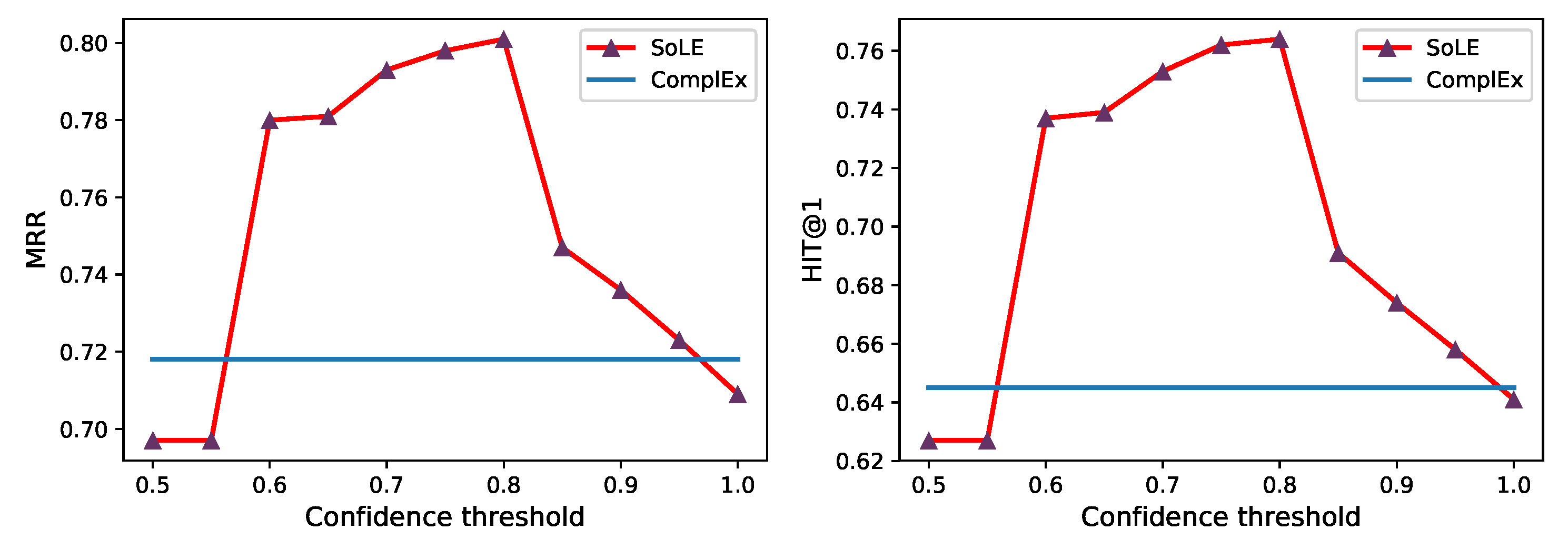
5.3.2. Influence of the Confidence Threshold

Here, we investigate how the confidence threshold influenced the performance of our method. We conducted the link prediction experiments on FB15K, where the hyper-parameters were fixed to the optimal configurations and the confidence thresholds were varied from 0.5 to 1.0 with an increment of 0.05. Figure 3 reports the results of MRR and HITS@1 achieved by SoLE with various thresholds. From the results, we can see that these two metrics had the same trend, and they both achieved the best performance when the threshold was 0.8. Thresholds higher than 0.8 will have a smaller number of rules, which can be extracted in the grounding generation stage, while ones lower than that might introduce too many less credible rules. Therefore, after the threshold exceeded 0.8, the performance decreased when the threshold grew, and after it was lower than that, the performance also decreased when the threshold decreased. Based on this observation, we assigned the confidence threshold to 0.8 in SoLE and obtained the best performance.

5.3.3. Comparison of Forward Chaining and One Time Inference

We further investigated the effectiveness of forward chaining by comparing it with one time inference. Since a small amount of rules was extracted from the dataset DB100K and the groundings generated by forward chaining and one time inference were the same, we only conducted the comparison experiment on FB15K. Table 4 shows the results achieved by SoLE with one time inference and forward chaining. From the results, we can observe that forward chaining slightly, but not statistically significantly outperformed one time inference.

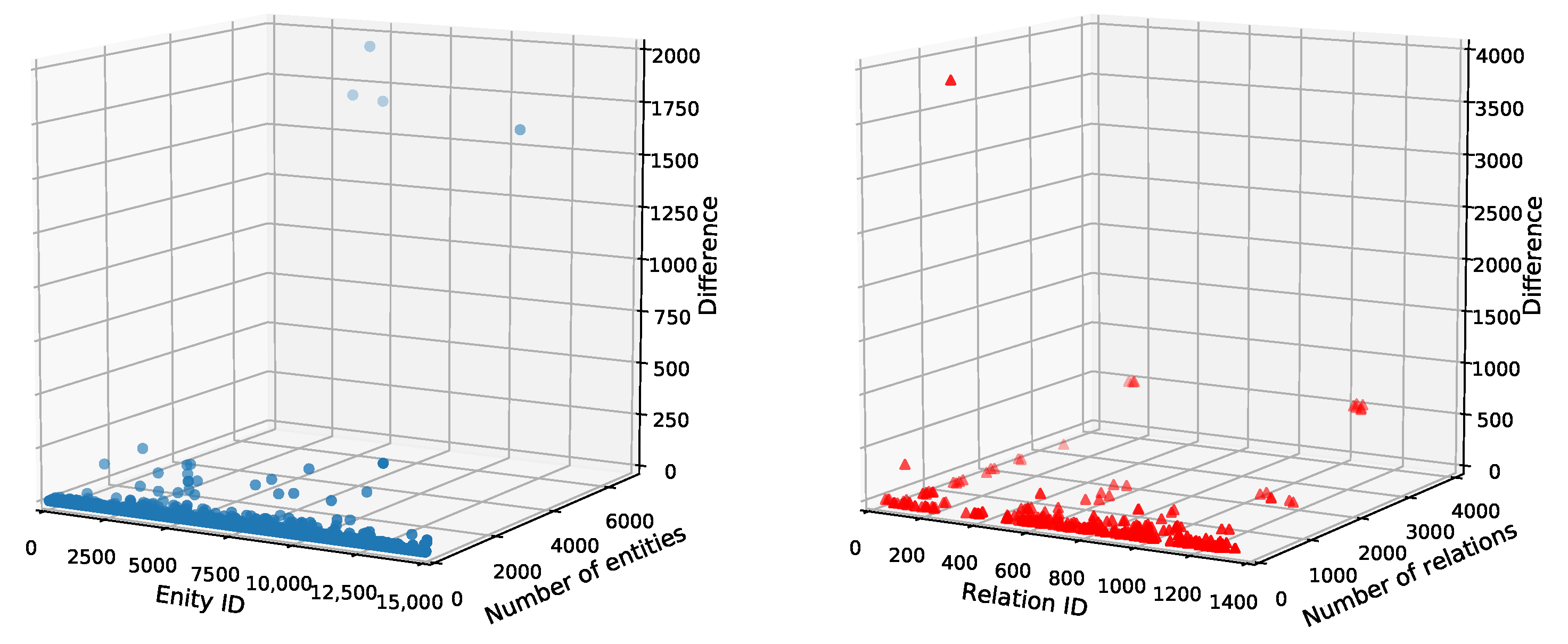
In order to figure out why the improvement was not obvious, we analyzed the different groundings generated by forward chaining and one time inference. We mainly explored the conclusions of the groundings that indicated the new derived triples. Figure 4 depicts the distributions of entities and relations in the conclusions. The X-axis denotes the entity/relation ID used in our code representing entities/relations; the Y-axis denotes the number of the entities/relations involved in the conclusions of the groundings generated by one time inference; and the Z-axis denotes the difference between the number of the entities/relations from forward chaining and the ones from one time inference. In the left picture of Figure 4, four entities, each one had a large number in the groundings generated by one time inference, accounting for 32% of the total difference, and 92% of 13,537 entities in the conclusions had the difference value less than one. Meanwhile, in the right picture, 14 out of 299 relations in the conclusions accounted for 99.99% of the total differences when they already had a large number in the conclusions w.r.t. one time inference.

These data indicated that most of the entities and relations in the more derived triples from forward chaining had already shown up quite a few times in the conclusions of the groundings from one time inference where they may have contributed to learning good embeddings, while the embeddings of other entities and relations may not be improved too much because of their same low frequencies.

Though the improvement was not significant, forward chaining indeed helped learn better embeddings. We took out 14 relations from the groundings, which accounted for the mostly differences, and obtained the link prediction results on the test sets of FB15K only containing these relations.

Table 5. Fourteen relations from FB15K, which account for the most differences shown in the right picture of Figure 4.

Relations	/basketball/basketball_position/player_roster_position./sports/sports_team_roster/team
	/sports/sports_position/players./ice_hockey/hockey_roster_position/team
	/sports/sports_team/roster./ice_hockey/hockey_roster_position/position
	/sports/sports_position/players./baseball/baseball_roster_position/team
	/basketball/basketball_team/roster./sports/sports_team_roster/position
	/basketball/basketball_position/player_roster_position./basketball/basketball_roster_position/team
	/sports/sports_team/roster./basketball/basketball_roster_position/position
	/basketball/basketball_team/roster./basketball/basketball_roster_position/position
	/sports/sports_position/players./basketball/basketball_roster_position/team
	/baseball/baseball_team/current_roster./sports/sports_team_roster/position
	/sports/sports_team/roster./baseball/baseball_roster_position/position
	/base/aareas/schema/administrative_area/administrative_area_type
	/location/statistical_region/gni_in_ppp_dollars./measurement_unit/dated_money_value/currency
	/location/statistical_region/gni_per_capita_in_ppp_dollars./measurement_unit/dated_money_value/currency

gives these 14 relations, and

Table 6. Link prediction results achieved by SoLE_OTI and SoLE on the test sets of FB15K, which only contain the 14 relations given in Table 5.

Method	MRR	HITS@1	HITS@3	HITS@10
SoLE_OTI	0.809	0.792	0.802	0.854
SoLE	0.814	0.802	0.812	0.854

shows the results of link prediction. The results showed that forward chaining helped SoLE learn better embeddings for these relations even though many of them had shown up more than 3000 times in the groundings of SoLE_OTI. Furthermore, we chose the other three relations and constructed a query for each relation where its missing entity appeared more times in the groundings of SoLE than SoLE_OTI.

Table 7. Results of three specific queries (predictions) on FB15K. Boldface entities are the right answers according to the test sets.

Query	(San Bernardino,/base/biblioness/bibs_location/state,?)
Method	SoLE		SoLE_OTI
Top 5 entities and their scores	California	0.793200	San Bernardino County	0.688559
	San Bernardino County	0.560985	California	0.106467
	Oregon	0.131643	United States of America	0.105158
	United States of America	0.117618	Oregon	0.061081
	Washington	0.093031	Nevada	0.044814
Query	(National League sports league,/baseball/baseball_league/teams,?)
Method	SoLE		SoLE_OTI
Top 5 entities and their scores	Colorado Rockies	0.967590	Milwaukee Brewers	0.945655
	Houston Astros	0.967565	Houston Astros	0.904532
	Montreal Expos	0.632854	Cleveland Indians	0.826663
	Milwaukee Brewers	0.506580	Baltimore Orioles	0.728855
	Oakland Athletics	0.476932	Colorado Rockies	0.708710
Query	(?,/finance/currency/countries_used,Austria)
Method	SoLE		SoLE_OTI
Top 5 entities and their scores	Euro	0.446783	Chris Martin	0.321364
	Screen Actors Guild Award for Outstanding Performance by a Cast in a Motion Picture	0.303476	Nick Cannon	0.243579
	/m/0bs0bh	0.250963	Salzburg	0.113729
	sailing	0.214201	Miami	0.112626
	record producer	0.075033	Euro	0.084402

shows these queries and the results after performing the queries. From the top five entities and their scores in the results, we can observe that SoLE not only obtained the right entity as the first rank, but it also had a higher score than SoLE_OTI. The above analysis demonstrated the superiority of forward chaining to one time inference.

5.3.4. Runtime and Convergence

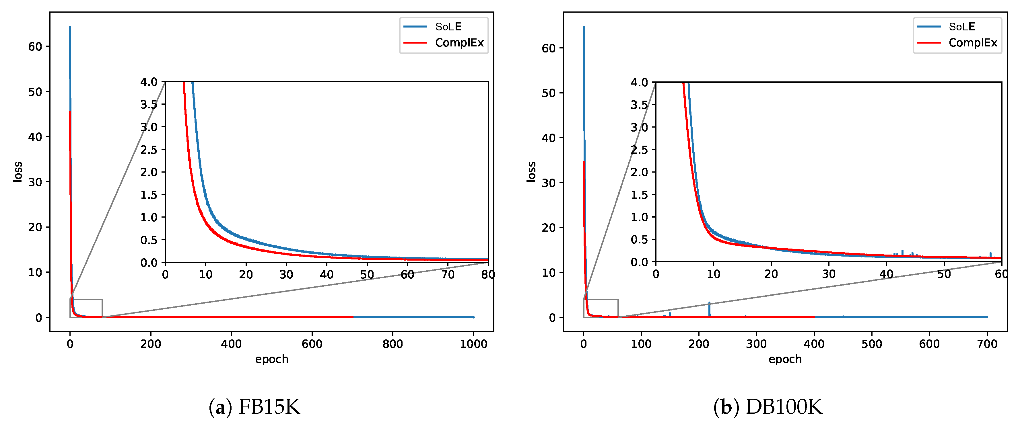
At last, we discuss the runtime of SoLE and the convergence of the training process in the embedding learning stage. Figure 5a,b shows the convergence of SoLE on FB15K and DB100K, respectively, compared to ComplEx. We can see that the convergence times of ComplEx and SoLE were very close, both around 50 epochs on FB15K and 40 epochs on DB100K, respectively, which indicated that integrating additional rules would not affect the convergence of the training process too much.

Table 8. Runtime on FB15K and DB100K. “Grnd. Gen.” is the time required for the Grounding Generation stage, and “Em. Learn.” for training per epoch.

	FB15K			DB100K
Method	Grnd. Gen. (s)	Em. Learn. (s/epoch)		Grnd. Gen. (s)	Em. Learn. (s/epoch)
ComplEx	-	8.64		-	9.74
SoLE	39.37	17.79		19.52	21.47

lists the runtime of SoLE required for its two stages and ComplEx required for model training on FB15K and DB100K. The training time per epoch of SoLE was approximately two times longer than ComplEx, since SoLE computed the additional gradient of the loss function for soft rules. Besides, we can see that the grounding generation stage of SoLE was quite efficient and cost very little time considering the whole runtime.

6. Conclusions and Future Work

This paper proposed Soft Logical Rules enhanced Embedding (SoLE), a novel paradigm of KG embedding, which was enhanced with a joint training algorithm that learned entity and relation embeddings using both soft rules and KG facts simultaneously, as well as forward chaining inference over logical rules to generate more valid groundings. Specifically, SoLE contained two stages: grounding generation and embedding learning. In the first stage, we extracted soft rules with certain confidences via modern rule mining system and then used the rule engine to perform forward chaining inference over these soft rules and KG facts to generate more groundings. At the stage of embedding learning, we devised a joint training algorithm to optimize over both KG facts and soft rules simultaneously where groundings of soft rules were modeled by t-norm fuzzy logics and soft rules were modeled by their corresponding groundings. The truth values calculated by the groundings were used to estimate soft rules, where the confidence of one soft rule was treated as the probability it held. SoLE then amounted to minimizing a global loss over both the loss function for KG facts and the L2 loss for soft rules. In this manner, the facts in groundings could capture the logical background knowledge in these rules so as to learn better embeddings. To sum up, this paper devised a novel joint training algorithm that directly injected the background knowledge of soft rules into embeddings and introduced forward chaining to KG embedding model with logical rules. Experimental results on benchmark KGs showed that our method achieved consistent improvements over the state-of-the-art baselines.

This research brought up some questions in need of further investigation. Firstly, our method could only support the Horn clause rules, which exclude negative atoms. Some other types of logical rules, such as $\forall x,y,z:(\mathrm{x},\mathrm{child}\_\mathrm{of},\mathrm{y})\wedge \neg (\mathrm{y},\mathrm{nationality},\mathrm{z})\Rightarrow \neg (\mathrm{x},\mathrm{nationality},\mathrm{z})$, cannot be extracted and performed by our method since KG does not contain negative triples. Secondly, our method may not be suitable for the extremely large scale KG with a large amount of relations and facts. Given this kind of KG, massive rules would be extracted, and the cost for performing forward chaining would be intolerant due to the high degree of space and time complexity. For future work, we would like to investigate the possibility of modeling all kinds of soft rules using only relation embeddings to avoid grounding, which might be space and time inefficient with regard to the extremely large scale KG.

References

- Miller, G.A. WordNet: A lexical database for English. Commun. ACM 1995, 38, 39–41. [Google Scholar] [CrossRef]
- Bollacker, K.; Evans, C.; Paritosh, P.; Sturge, T.; Taylor, J. Freebase: A collaboratively created graph database for structuring human knowledge. In Proceedings of the 2008 ACM SIGMOD International Conference on Management of Data, Vancouver, BC, Canada, 9–12 June 2008; pp. 1247–1250. [Google Scholar]
- Lehmann, J.; Isele, R.; Jakob, M.; Jentzsch, A.; Kontokostas, D.; Mendes, P.N.; Hellmann, S.; Morsey, M.; Van Kleef, P.; Auer, S.; et al. DBpedia—A large-scale, multilingual knowledge base extracted from Wikipedia. Semant. Web 2015, 6, 167–195. [Google Scholar] [CrossRef] [Green Version]
- Carlson, A.; Betteridge, J.; Kisiel, B.; Settles, B.; Hruschka, E.R.; Mitchell, T.M. Toward an architecture for never-ending language learning. In Proceedings of the Twenty-Fourth AAAI Conference on Artificial Intelligence, Atlanta, GA, USA, 11–15 July 2010. [Google Scholar]
- Cui, W.; Xiao, Y.; Wang, H.; Song, Y.; Hwang, S.W.; Wang, W. KBQA: Learning question answering over QA corpora and knowledge bases. Proc. VLDB Endow. 2017, 10, 565–576. [Google Scholar] [CrossRef] [Green Version]
- Hoffmann, R.; Zhang, C.; Ling, X.; Zettlemoyer, L.; Weld, D.S. Knowledge based weak supervision for information extraction of overlapping relations. In Proceedings of the 49th Annual Meeting of the Association for Computational Linguistics: Human Language Technologies, Portland, OR, USA, 19–24 June 2011; pp. 541–550. [Google Scholar]
- Zhang, F.; Yuan, N.J.; Lian, D.; Xie, X.; Ma, W.Y. Collaborative knowledge base embedding for recommender systems. In Proceedings of the 22nd ACM SIGKDD international conference on knowledge discovery and data mining, San Francisco, CA, USA, 13–17 August 2016; pp. 353–362. [Google Scholar]
- Ai, Q.; Azizi, V.; Chen, X.; Zhang, Y. Learning Heterogeneous Knowledge Base Embeddings for Explainable Recommendation. Algorithms 2018, 11, 137. [Google Scholar] [CrossRef] [Green Version]
- Lin, Y.; Liu, Z.; Sun, M.; Liu, Y.; Zhu, X. Learning entity and relation embeddings for knowledge graph completion. In Proceedings of the Twenty-ninth AAAI conference on artificial intelligence, Austin, TX, USA, 25–30 January 2015; pp. 2181–2187. [Google Scholar]
- De Assis Costa, G.; De Oliveira, J.M.P. A Relational Learning Approach for Collective Entity Resolution in the Web of Data. In Proceedings of the 5th International Conference on Consuming Linked Data, Riva del Garda, Italy, 19–21 October 2014. [Google Scholar]
- Weston, J.; Bordes, A.; Yakhnenko, O.; Usunier, N. Connecting Language and Knowledge Bases with Embedding Models for Relation Extraction. arXiv 2013, arXiv:1307.7973. [Google Scholar]
- Minervini, P.; Costabello, L.; Muñoz, E.; Nováček, V.; Vandenbussche, P.Y. Regularizing knowledge graph embeddings via equivalence and inversion axioms. In Joint European Conference on Machine Learning and Knowledge Discovery in Databases; Springer: Cham, Switzerland, 2017; pp. 668–683. [Google Scholar]
- Ding, B.; Wang, Q.; Wang, B.; Guo, L. Improving Knowledge Graph Embedding Using Simple Constraints. In Proceedings of the 56th Annual Meeting of the Association for Computational Linguistics (Volume 1: Long Papers), Melbourne, Australia, 15–20 July 2018; pp. 110–121. [Google Scholar]
- Guo, S.; Wang, Q.; Wang, L.; Wang, B.; Guo, L. Knowledge graph embedding with iterative guidance from soft rules. In Proceedings of the Thirty-Second AAAI Conference on Artificial Intelligence, New Orleans, LA, USA, 2–7 February 2018. [Google Scholar]
- Nguyen, D.Q. An overview of embedding models of entities and relationships for knowledge base completion. arXiv 2017, arXiv:1703.08098. [Google Scholar]
- Wang, Q.; Mao, Z.; Wang, B.; Guo, L. Knowledge graph embedding: A survey of approaches and applications. IEEE Trans. Knowl. Data Eng. 2017, 29, 2724–2743. [Google Scholar] [CrossRef]
- Bordes, A.; Usunier, N.; Garcia-Duran, A.; Weston, J.; Yakhnenko, O. Translating embeddings for modeling multi-relational data. In Proceedings of the Advances in Neural Information Processing Systems, Lake Tahoe, NV, USA, 5–10 December 2013; pp. 2787–2795. [Google Scholar]
- Trouillon, T.; Welbl, J.; Riedel, S.; Gaussier, É.; Bouchard, G. Complex embeddings for simple link prediction. In Proceedings of the International Conference on Machine Learning, New York, NY, USA, 19–24 June 2016; pp. 2071–2080. [Google Scholar]
- Dettmers, T.; Minervini, P.; Stenetorp, P.; Riedel, S. Convolutional 2d knowledge graph embeddings. In Proceedings of the Thirty-Second AAAI Conference on Artificial Intelligence, New Orleans, LA, USA, 2–7 February 2018. [Google Scholar]
- Wang, Q.; Wang, B.; Guo, L. Knowledge base completion using embeddings and rules. In Proceedings of the Twenty-Fourth International Joint Conference on Artificial Intelligence, Buenos Aires, Argentina, 25–31 July 2015. [Google Scholar]
- Wei, Z.; Zhao, J.; Liu, K.; Qi, Z.; Sun, Z.; Tian, G. Large-scale knowledge base completion: Inferring via grounding network sampling over selected instances. In Proceedings of the 24th ACM International on Conference on Information and Knowledge Management, Melbourne, Australia, 19–23 October 2015; pp. 1331–1340. [Google Scholar]
- Rocktäschel, T.; Singh, S.; Riedel, S. Injecting logical background knowledge into embeddings for relation extraction. In Proceedings of the 2015 Conference of the North American Chapter of the Association for Computational Linguistics: Human Language Technologies, Denver, CO, USA, 31 May–5 June 2015; pp. 1119–1129. [Google Scholar]
- Guo, S.; Wang, Q.; Wang, L.; Wang, B.; Guo, L. Jointly embedding knowledge graphs and logical rules. In Proceedings of the 2016 Conference on Empirical Methods in Natural Language Processing, Austin, TX, USA, 1–5 November 2016; pp. 192–202. [Google Scholar]
- Demeester, T.; Rocktäschel, T.; Riedel, S. Lifted Rule Injection for Relation Embeddings. In Proceedings of the 2016 Conference on Empirical Methods in Natural Language Processing, Austin, TX, USA, 1–5 November 2016; pp. 1389–1399. [Google Scholar]
- Minervini, P.; Demeester, T.; Rocktäschel, T.; Riedel, S. Adversarial sets for regularising neural link predictors. In Proceedings of the 33rd Conference on Uncertainty in Artificial Intelligence, Sydney, Australia, 11–15 August 2017; pp. 1–10. [Google Scholar]
- Zhang, W.; Paudel, B.; Wang, L.; Chen, J.; Zhu, H.; Zhang, W.; Bernstein, A.; Chen, H. Iteratively Learning Embeddings and Rules for Knowledge Graph Reasoning. In Proceedings of the World Wide Web Conference, San Francisco, CA, USA, 13–17 May 2019; pp. 2366–2377. [Google Scholar]
- Qu, M.; Tang, J. Probabilistic Logic Neural Networks for Reasoning. arXiv 2019, arXiv:1906.08495. [Google Scholar]
- Galarraga, L.; Teflioudi, C.; Hose, K.; Suchanek, F.M. Fast rule mining in ontological knowledge bases with AMIE. Very Large Data Bases 2015, 24, 707–730. [Google Scholar] [CrossRef] [Green Version]
- Proctor, M. Drools: A Rule Engine for Complex Event Processing. In Proceedings of the 4th International Conference on Applications of Graph Transformations with Industrial Relevance, Budapest, Hungary, 4–7 October 2011. [Google Scholar]
- Forgy, C.L. Rete: A fast algorithm for the many pattern/many object pattern match problem. Artif. Intell. 1982, 19, 17–37. [Google Scholar] [CrossRef]
- Hájek, P. Metamathematics of Fuzzy Logic; Springer: Berlin, Germany, 2013; Volume 4. [Google Scholar]
- Kingma, D.P.; Ba, J. Adam: A method for stochastic optimization. arXiv 2014, arXiv:1412.6980. [Google Scholar]
- Yang, B.; Yih, W.T.; He, X.; Gao, J.; Deng, L. Embedding entities and relations for learning and inference in knowledge bases. arXiv 2014, arXiv:1412.6575. [Google Scholar]
- Liu, H.; Wu, Y.; Yang, Y. Analogical inference for multi-relational embeddings. In Proceedings of the 34th International Conference on Machine Learning-Volume 70. JMLR. org, Sydney, Australia, 6–11 August 2017; pp. 2168–2178. [Google Scholar]
- Schlichtkrull, M.; Kipf, T.N.; Bloem, P.; Van Den Berg, R.; Titov, I.; Welling, M. Modeling relational data with graph convolutional networks. In Proceedings of the European Semantic Web Conference, Crete, Greece, 3–7 June 2018; pp. 593–607. [Google Scholar]
Figure 1.
An illustration of one time logical inference and forward chaining inference over given rules and a simple KG, which was adapted from Dat Quoc Nguyen [15].
Figure 2.
Overview of the Soft Logical rules enhanced Embedding (SoLE) framework. KG, Knowledge Graph.
Figure 3.
Results of MRR (left) and HITS@1 (right) achieved by SoLE with different confidence thresholds on the test set of FB15K.
Figure 4.
The distributions of entities (left) and relations (right) in the conclusions of the groundings generated by forward chaining and one time inference.
Figure 5.
Convergence times of embedding learning in ComplEx and SoLE on datasets FB15K and DB100K, respectively.