Uncertainty Quantification Approach on Numerical Simulation for Supersonic Jets Performance

Abstract

One of the main issues addressed in any engineering design problem is to predict the performance of the component or system as accurately and realistically as possible, taking into account the variability of operating conditions or the uncertainty on input data (boundary conditions or geometry tolerance). In this paper, the propagation of uncertainty on boundary conditions through a numerical model of supersonic nozzle is investigated. The evaluation of the statistics of the problem response functions is performed following ‘Surrogate-Based Uncertainty Quantification’. The approach involves: (a) the generation of a response surface starting from a DoE in order to approximate the convergent–divergent ‘physical’ model (expensive to simulate), (b) the application of the UQ technique based on the LHS to the meta-model. Probability Density Functions are introduced for the inlet boundary conditions in order to quantify their effects on the output nozzle performance. The physical problem considered is very relevant for the experimental tests on the UQ approach because of its high non-linearity. A small perturbation to the input data can drive the solution to a completely different output condition. The CFD simulations and the Uncertainty Quantification were performed by coupling the open source Dakota platform with the ANSYS Fluent^® CFD commercial software: the process is automated through scripting. The procedure adopted in this work demonstrate the applicability of advanced simulation techniques (such as UQ analysis) to industrial technical problems. Moreover, the analysis highlights the practical use of the uncertainty quantification techniques in predicting the performance of a nozzle design affected by off-design conditions with fluid-dynamic complexity due to strong nonlinearity.

1. Introduction

In recent years, an important part of the research in numerical simulations, in many engineering sectors, has been dedicated to the performance prediction of systems and components in off-design conditions. The behavior of a system or a component in conditions different from those for which it was designed is not only related to the deterministic variation of the input parameters, but also to the aleatory uncertainty which can characterize the input data and the geometrical tolerances. Hence, in order to improve the accuracy and the reliability of the numerical predictions, it is necessary to understand how the uncertainties can affect the results of the problem under investigation. This is one of the main targets of Uncertainty Quantification (UQ) analysis with direct positive fall-out on engineering problems. Computational Fluid Dynamics (CFD) is one of the disciplines where UQ is increasingly applied within a simulation environment. The UQ analysis is becoming an effective approach for industrial use thanks to the concurrent development of both soft-computing methods and computer performance. The use of CFD coupled to optimization algorithms for the automatic design optimization of industrial components is nowadays a mature technology [1,2]. More recently, the development of Response Surface Methodology (RSM) has significantly enhanced the effectiveness of the design optimization based on simulation [3,4], as an industrial standard or for data mining and diagnostic applications [5,6]. The same RSM approach can be used to develop very efficient frameworks for UQ analysis [7]. A contribution to this field is given in the paper with reference to one of the most interesting examples of compressible flow thanks to its high non-linearity: the adiabatic flow in a variable section duct. It is a relevant case for its physical and mathematical background, and it has also a wide range of engineering applications. The best known application is for spacecraft propulsion in aircraft engines or in supersonic wind tunnel [8]. Convergent–divergent nozzles are also applied in gas burners [9,10] and in supersonic water separators for natural gas purification [11,12]. The preliminary design of a supersonic nozzle (De Laval nozzle) is based on the basic gas-dynamic equations in order to have a reference, ideal, operative condition of a fully expanded jet [8]. However, the theory is based on some assumptions, such as isentropic flow conditions, that can affect the actual nozzle performance. Moreover, the real operating conditions (pressure, temperature, gas mixture composition, etc.) can cause a significant change in the flow structure and in the shock waves generation with direct outcomes on nozzle performance.

The main goal of this paper is to answer to the following questions: a small variation of some input parameters can remarkably affect the performance of a designed convergent–divergent nozzle? Can UQ methods help to quantify the above effect and give more insight into the nozzle behavior?

The uncertainties propagation through the CFD model of the nozzle was performed using an automated procedure developed by the authors within the Dakota open source platform. The UQ approach is a ‘surrogate-based’ approach: a response surface was generated from a DoE, and then, the Latin Hypercube Sampling (LHS) was applied to the meta-model to perform the UQ analysis. The use of a surrogate model is highly effective in reducing calculation times when a sampling-based UQ method is used: in this case, in fact, a high number of response function evaluations is required to generate converging statistics.

The LHS was performed both for the DoE generation and for the UQ analysis. In LHS, the design space (with dimensions equal to the problem variables) is subdivided into an orthogonal grid with N elements per parameter. Within the grid, N sub-volumes are located so that along each row and column of the grid, only one sub-volume is chosen. Inside each sub-volume, a sample is chosen randomly [13]. The LHS method is widely used because it ensures a better coverage of the design space [14,15,16,17] and a faster convergence with respect to the basic Monte Carlo method.

The surrogate model was generated through the Gaussian Process (also known as Kriging) approach which uses a Gaussian correlation function with parameters that are selected by Maximum Likelihood Estimation (MLE); this correlation function results in a response surface that is ${\mathrm{C}}^{\infty }$ continuous [14].

In a first application, an optimized nozzle geometry with air flowing at a supersonic Mach number was considered. The commercial software ANSYS Fluent^® was used to generate a series of CFD simulations to identify the influence of the nozzle discharge pressure on the convergent–divergent operating condition, flow structure and performance. A perturbation range of the exit static pressure was chosen with respect to the critical gas-dynamic condition, where the normal shock wave is positioned at the nozzle exit section (referred to the r2 condition in classical literature). The choice of this particular condition is related to the potential performance drop that will occur if the shock wave moves into the divergent part of the nozzle. After a preliminary sensitivity analysis, a full UQ approach was developed to quantify the effects of the input variable distribution (ambient static pressure) on the nozzle performance.

A second application considers the flow of natural gas in a convergent–divergent nozzle to understand the effects of the gas chemical composition on the expansion nozzle performance. The gas composition variation can occur on a daily or seasonal base, according to the geographical area and pipeline used [18], and it is a serious problem for several industrial applications, where large quantities of natural gas are treated and energy consumption is an issue [19,20]. The same investigation approach was applied as for the first case and the effectiveness of the UQ analysis is confirmed.

2. CFD Model

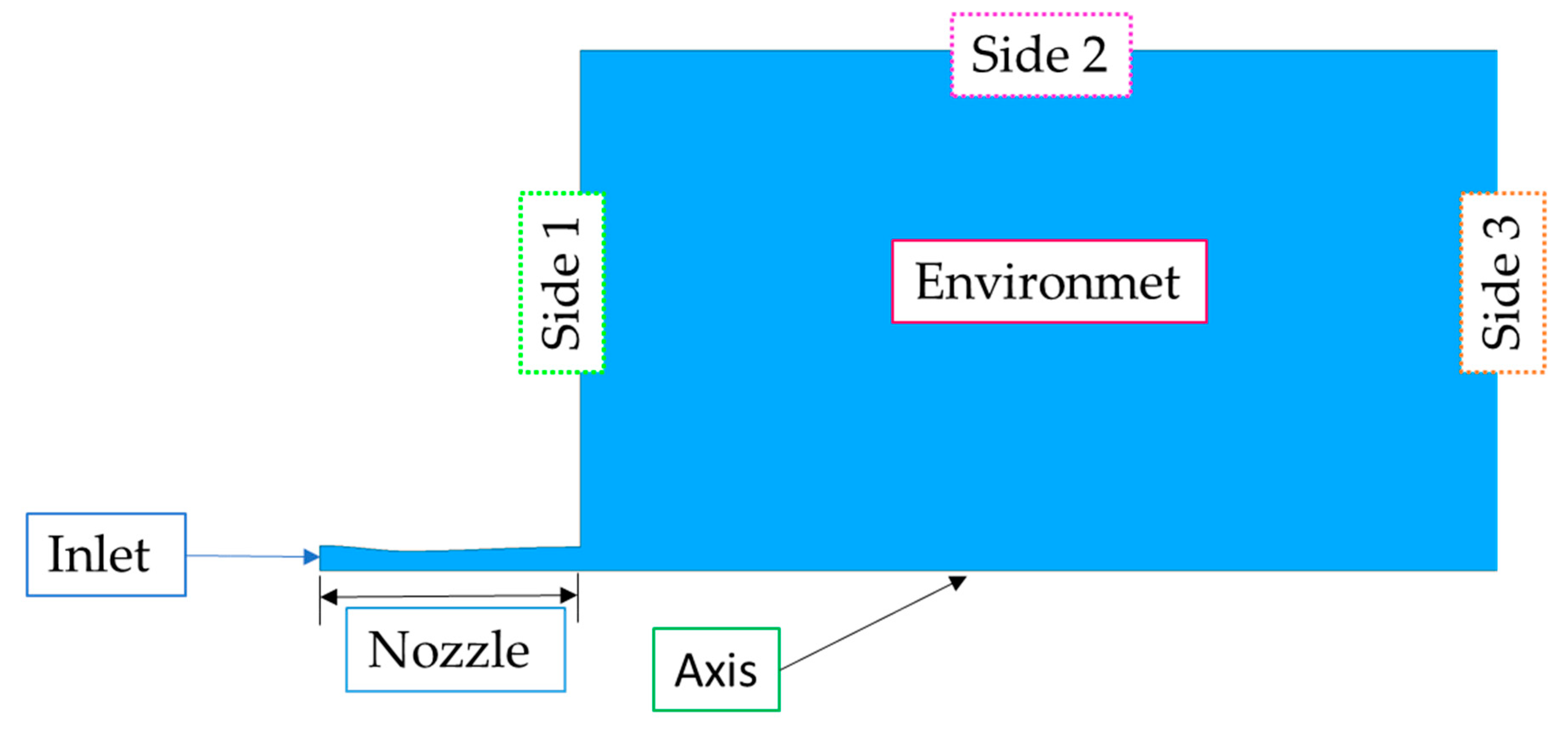
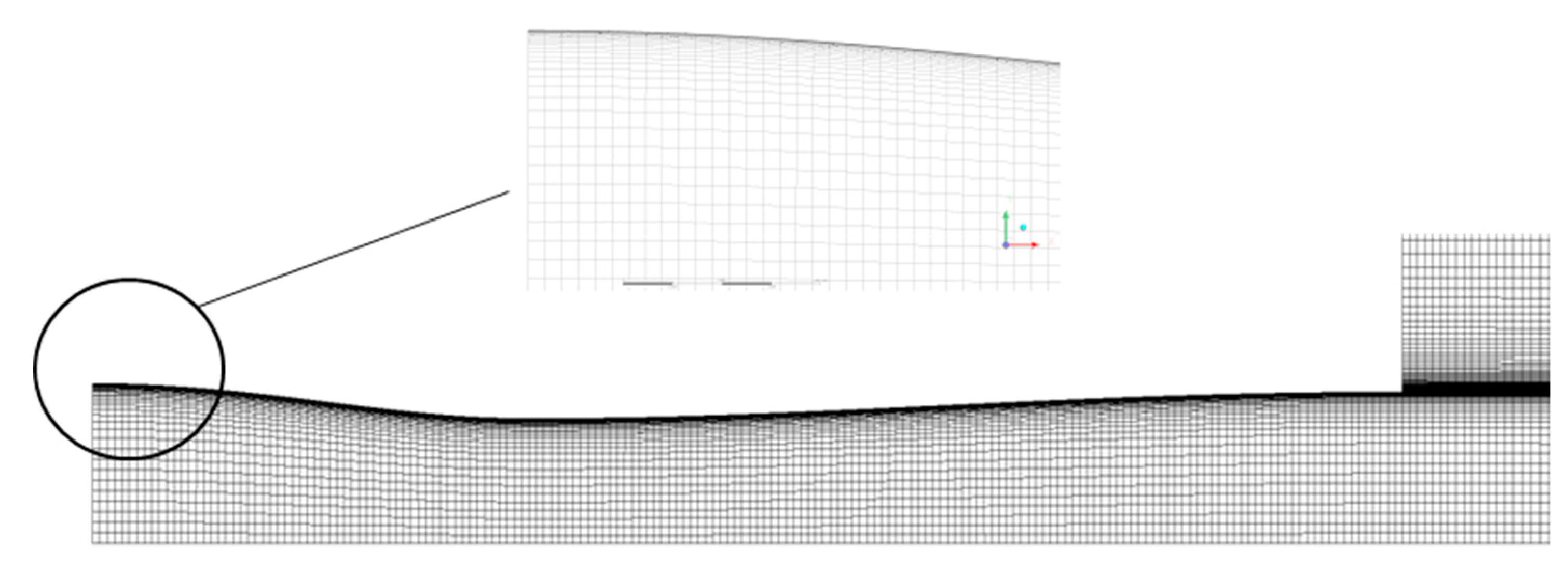
The fluid domain consists of a 2D axisymmetric De Laval nozzle with an “expansion volume” (Figure 1) at the exit, which represents the discharge environment at constant pressure. The axisymmetric RANS equations were solved using an ‘axis’ boundary condition at the nozzle axis, as common practice [21]. A structured grid was used for the spatial discretization. As shown in Figure 2, a grid refinement was performed near the nozzle wall, in order to ensure a y+ value close to one. The Reynolds Averaged Navier Stokes Equations (RANS) in the steady form are numerically solved with the addition equation for the turbulence closure. The two equation k-ω SST turbulence model is selected based on previous experience on the application case; it allows a good accuracy both in proximity and far from the walls. A second order upwind scheme was selected for the spatial discretization, because if the flow is not aligned with the structured mesh (e.g., oblique shock waves) the first-order convective discretization is not appropriate.

Table 1. Boundary conditions.

Domain Zone	Type
Nozzle Inlet	Total pressure; Total temperature
Environment Side walls	Discharge pressure
Nozzle walls	No slip condition; adiabatic

and Figure 1 summarize and show the set of boundary conditions used in the CFD simulations:

-

total pressure and total temperature at the nozzle inlet;

-

static pressure on expansion volume (outlet domain) side walls.

In the first part of the work, the operating fluid is air as an ideal compressible gas with constant Cp. Sutherland’s law with three coefficients (Equation (1)) is adopted to model the variation of viscosity with temperature.

$$\mu ={\mathsf{\mu }}_{\mathrm{ref}}{\left(\frac{T}{{\mathrm{T}}_{\mathrm{ref}}}\right)}^{\frac{3}{2}}\left(\frac{{\mathrm{T}}_{\mathrm{ref}}-\mathrm{S}}{T-\mathrm{S}}\right)$$

(1)

In the second part of the article, the working fluid is natural gas treated as an ideal and compressible gas and the viscosity is computed through Sutherland’s law with suitable coefficients for methane.

3. UQ Analysis on Nozzle Discharge Pressure

3.1. Sensitivity Analysis on Discharge Pressure

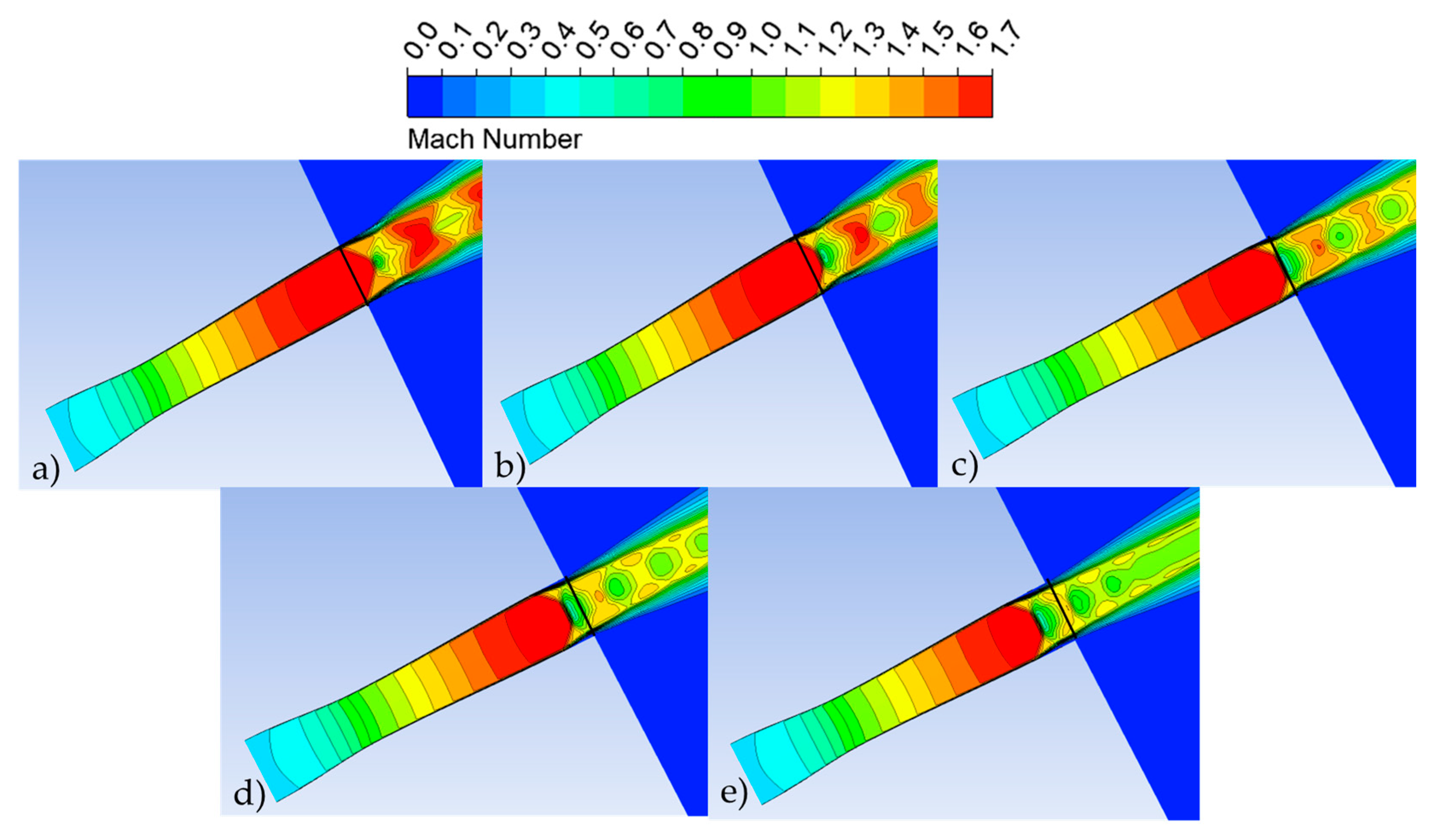
The value of the discharge pressure p_s has a remarkable impact on the nozzle flow structure, especially in determining the position and strength of the shock wave: this is evident referring to the ‘r2’ condition where the shock wave is positioned at the nozzle exit section [8]. As a proof of the reliability of the CFD model, similar results have been obtained in similar conditions in the experimental case by Zapryagaev et al. [22]. Figure 3 shows Mach number contours for five different p_s values (80 kPa ÷ 120 kPa) around the ‘r2’ condition. The flow structure and the shock wave location change significantly even with a small Δ of 10 kPa (about 10% of the pressure range mean value).

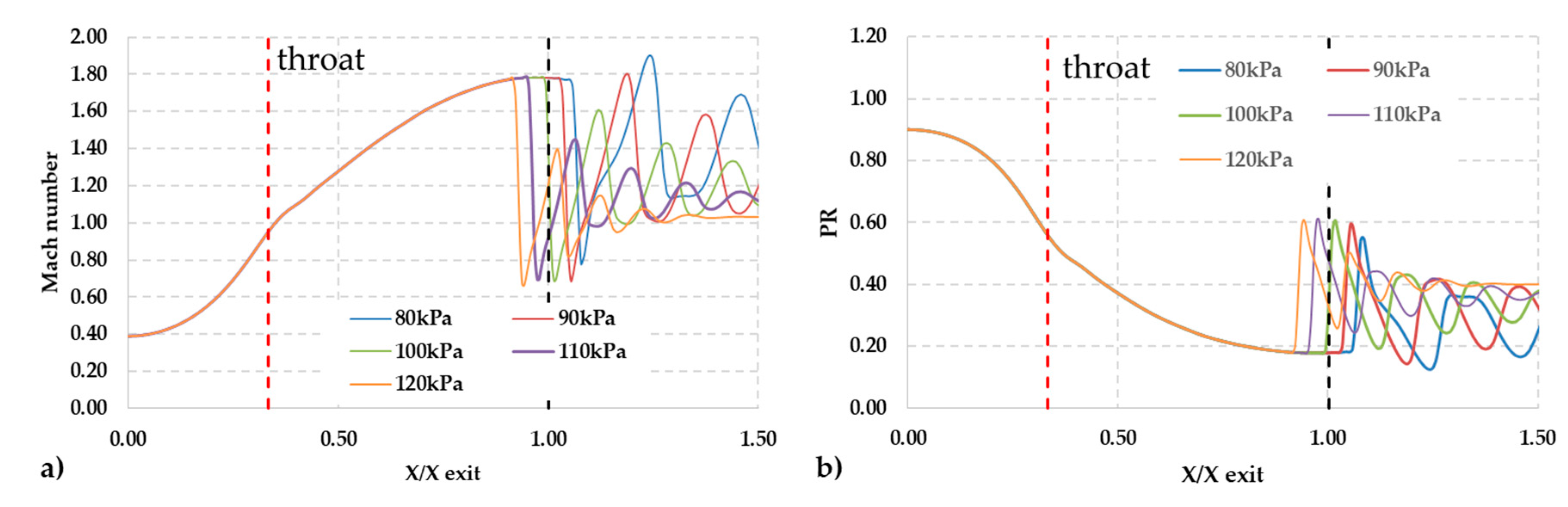
The performance variation of the nozzle within the above range is further confirmed by the charts in Figure 4, which represent the Mach and the Pressure Ratio (PR) along the nozzle axis (Equation (2)).

$$PR=p_s/{\mathrm{p}}_{\mathrm{t}\mathrm{in}}$$

(2)

It is evident that the position of the shock wave close to the nozzle exit is affected by the small change in the environment discharge static pressure. Another important parameter, which confirms the performance variation, is the Δp_t (Equation (3)) i.e., the total pressure drop through the nozzle that quantifies the mechanical losses due to viscous or compressible flow effects. In

Table 2. Total pressure drop values with respect to the operative condition.

CASE	Discharge Pressure (ps) [kPa]	Δpt [Pa]
1	80	19,270
2	90	20,145
3	100	31,926
4	110	32,675
5	120	34,972

, the large variation of this quantity was reported: losses tend to decrease with outlet static pressure in a non-linear way (see the difference between cases 1 and 2 compared to 2 and 3); this is related to the shock wave location (inside/outside the convergent–divergent).

$$\Delta p_t={\mathrm{p}}_{\mathrm{t}\mathrm{in}}-p_{t\mathrm{out}}$$

(3)

This off-design behavior makes the UQ analysis useful to study the component response to a non-deterministic input variable.

3.2. Uncertainty Quantification Analysis

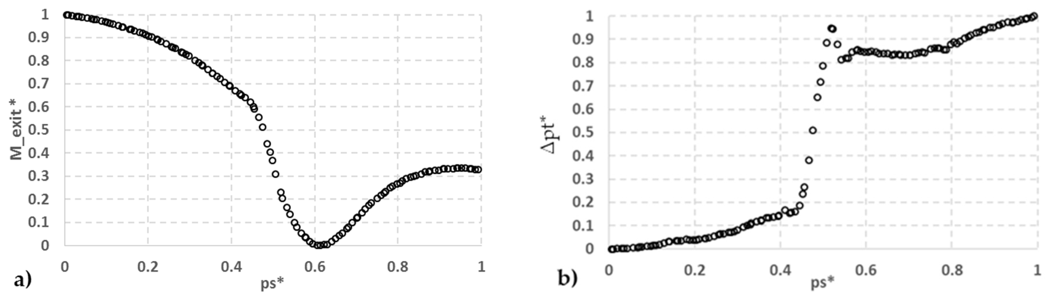
A UQ analysis was carried out considering the discharge pressure as the variable parameter. The Quantities of Interest (QoI) considered as output performance parameters are the Mach number at the nozzle exit (M_exit) and the total pressure drop (Δp_t). With a fully automated procedure implemented in the Dakota environment, a DoE for the two QoI based on LHS method was performed for the pressure range 80–120 [kPa]. The outlet static pressure values provided by Dakota, according to LHS scheme, were used as the input variable in Fluent CFD software, which allowed us to obtain the corresponding response functions values (see Figure 5). In order to approximate the ‘physical’ (numerical) model, 121 samples were chosen inside the design space. Equations (4)–(6) show the response functions in the normalized form:

$$p_s^{\ast }=\frac{p_s-{\mathrm{p}}_{\mathrm{s}\min }}{{\mathrm{p}}_{\mathrm{s}\max }-{\mathrm{p}}_{\mathrm{s}\min }}$$

(4)

$$M_{\mathrm{exit}}^{\ast }=\frac{M_{\mathrm{exit}}-{\mathrm{M}}_{\mathrm{exit}\min }}{{\mathrm{M}}_{\mathrm{exit}\max }-{\mathrm{M}}_{\mathrm{exit}\min }}$$

(5)

$$\Delta p_t^{\ast }=\frac{\Delta p_t-\Delta {\mathrm{p}}_{\mathrm{t}\min }}{\Delta {\mathrm{p}}_{\mathrm{t}\max }-\Delta {\mathrm{p}}_{\mathrm{t}\min }}$$

(6)

Kriging or ‘Gaussian Process’ Response Surface Methodology is considered and the response surfaces for the above functions were generated from the training points given by the DoE. The UQ analysis was then performed through Latin Hypercube sampling method, considering 1000 samples taken on the generated response surfaces.

In order to ensure the meta-model reliability, a cross-validation analysis was performed. In Dakota, the type of cross-validation which can be exploited is the k-fold cross-validation: at first, the DoE dataset is divided into k partitions and k meta-models are generated, each excluding the k-th partition of training data. Each surrogate is tested at the points that were excluded in its generation and the user-specified diagnostic metrics are computed with respect to the held out data [14]. In this work, a particular type of k-fold cross-validation was performed, i.e., the Leave-one-out cross-validation or Prediction Error Sum of Squares (PRESS). In this special case, the number of partitions is equal to the number of data points. The results obtained from this analysis, reported in

Table 3. Metrics for cross validation analysis of the response surfaces.

Metrics	Mexit	Δpt [Pa]
Root Mean Squared (RMS)	4.15 × 10−3	175.2
Mean Absolute Value	2.84 × 10−3	97.9
Maximum Absolute Value	1.70 × 10−2	739.7

, include the Root Mean Squared, the Mean Absolute Value and the Maximum Absolute Value of the prediction error (calculated between the observed value and the surrogate model prediction for the training data points).

Moreover, three random operating points were selected from the UQ database of 1000 samples, and then, simulated with the CFD solver. The corresponding fluid dynamics results for the QoI were given in input to Dakota as a challenge set of data. The metrics calculated with respect to this dataset are reported in

Table 4. Metrics for challenge data.

Metrics	Mexit	Δpt [Pa]
Root Mean Squared (RMS)	5.06 × 10−4	189.7
R squared	0.998411	0.97978
Mean Absolute Value	4.57 × 10−4	119.2
Maximum Value	7.00 × 10−4	327.9

.

The outcomes of the previous analyses were supplemented by the calculation of the relative percentage error (

Table 5. Relative percentage error between CFD and response surfaces values for random samples.

ps [Pa]	Percentage Error Mexit	Percentage Error Δpt
80,870	0.043%	−0.053%
100,451	0.015%	0.964%
117,848	0.042%	−0.056%

) between the CFD and the surrogate model response function values. The obtained results certify the reliability of the meta-model.

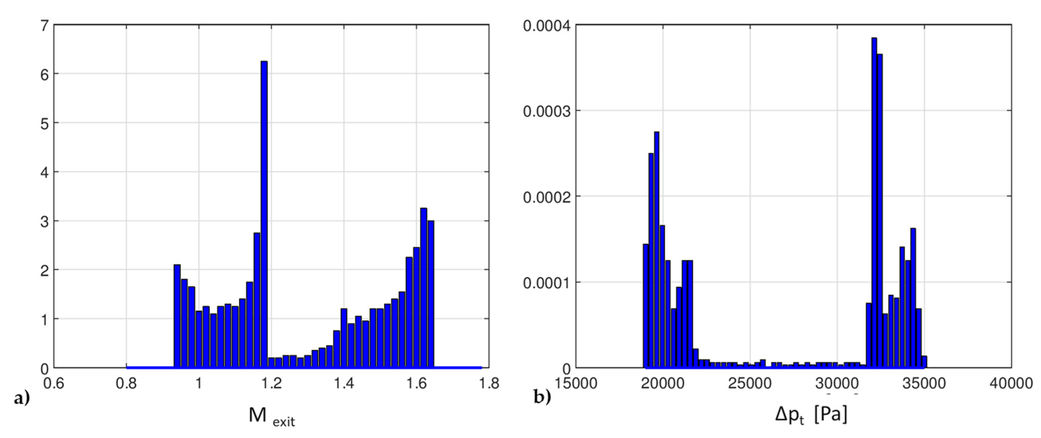
At first, a uniform distribution of the p_s variable were considered as the input probability density function (pdf): in this case, any pressure values within the established range have the same probability. Results of the uncertainty propagation through the surrogate model are the output functions (M_exit and Δp_t) discretized pdfs, reported in Figure 6. It is evident that the pdfs of the QoI are very far from the uniform distribution of the input variable (p_s). The physical explanation of these non-uniform pdfs can be found, considering that the ‘r2’ state matches with the case p_s = 100 [kPa], i.e., the mean of the uncertain input variable distribution. Around this value, two kinds of solutions are highly probable, as evidenced by the exit Mach and Δp_t pdfs (Figure 6):

• high exit Mach and low losses → overexpanded jet with shock waves outside the nozzle;
• low exit Mach and high losses → shock waves inside the nozzle.

This means that even with a large variation of the input variable, the most frequent flow structures can be restricted to two main ranges of M _exit and Δp_t.

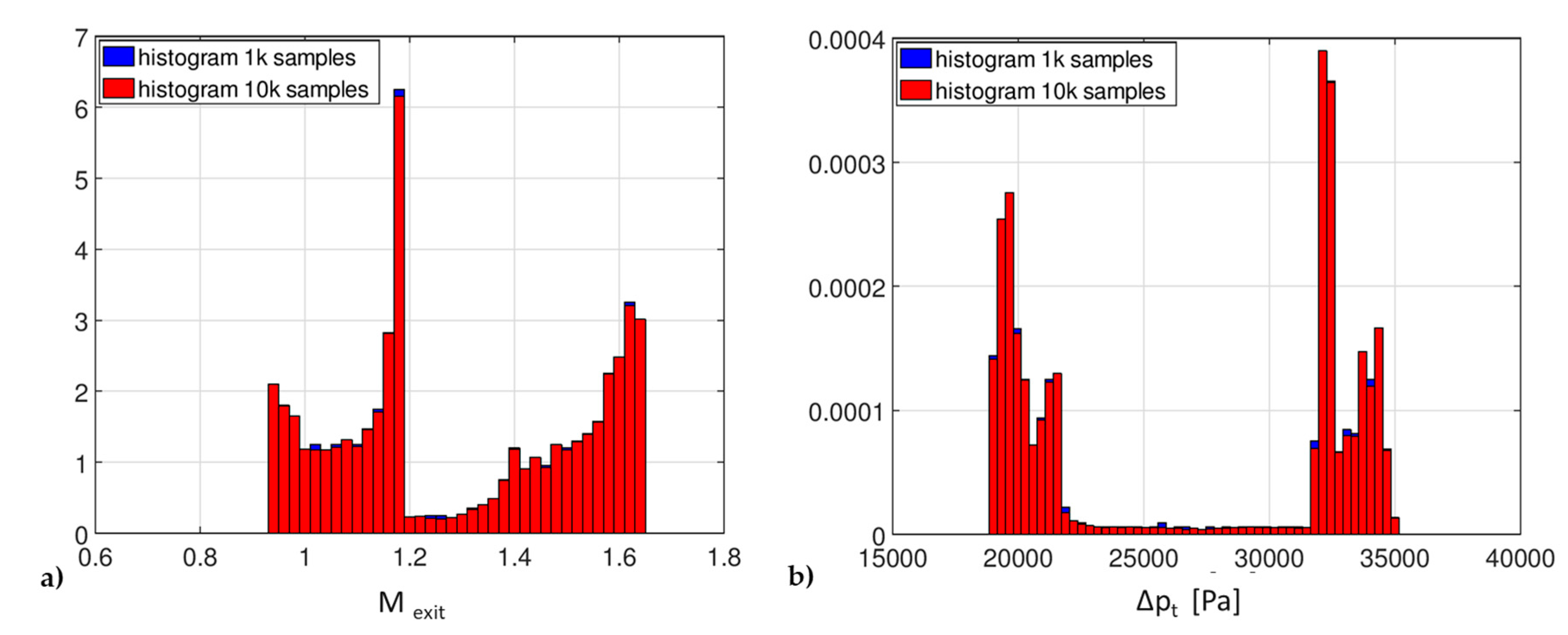
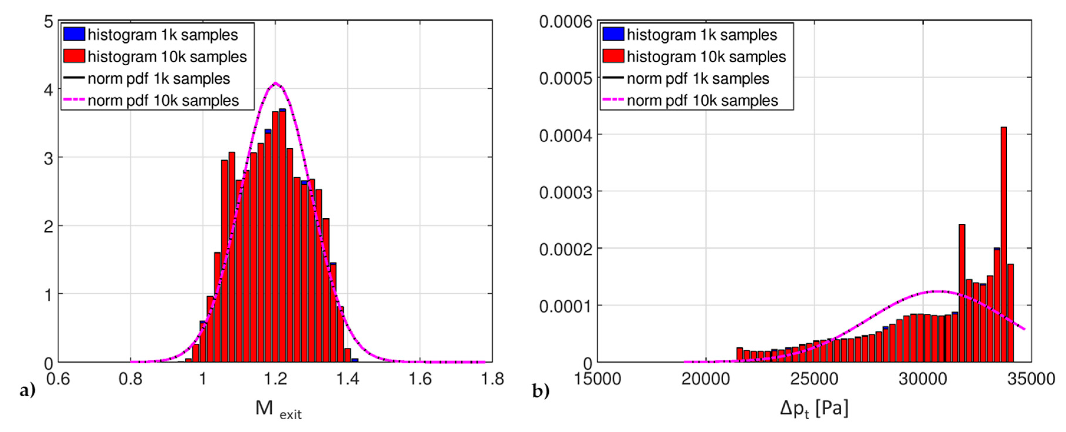
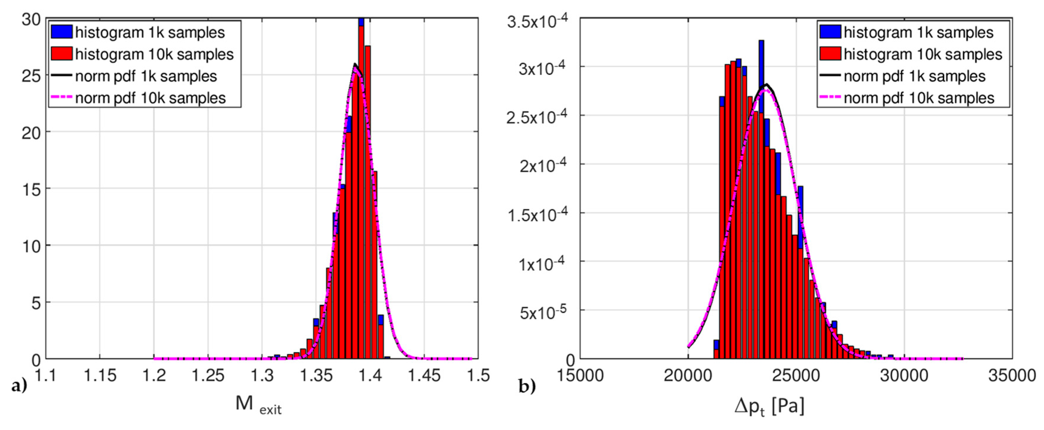
In order to provide more reliable results for the UQ analysis, a second case with an increased number of samples (10,000, one order of magnitude greater than the previous one) was considered. The comparison among the histograms obtained for the QoI is reported in Figure 7: differences between the two distributions can be detected, but they are so small that the 1000 samples UQ analysis can be considered satisfactory.

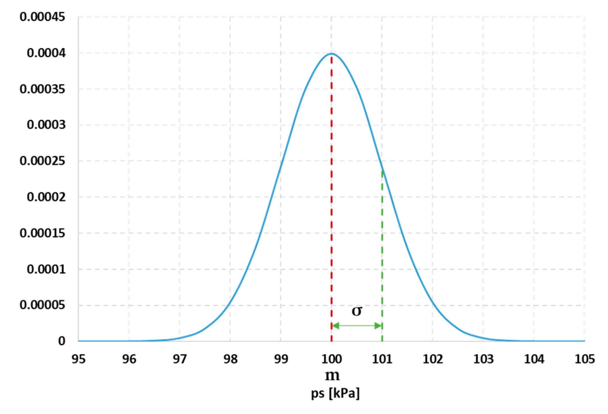
Another case was performed, assigning a normal distribution for the input pdf with a mean value ‘m’ (100 [kPa]) centered on the previously considered variation range and a standard deviation σ chosen in order to have a small perturbation of the pressure: e.g., σ ≈ 1% of the mean value. The resulting pdf for the input variable ps is shown in Figure 8.

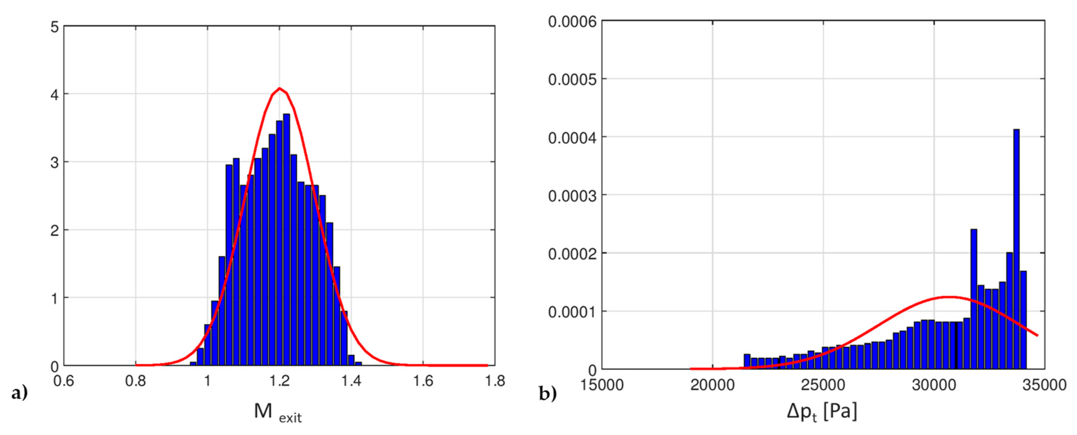
Using again the LHS method for the uncertainty quantification propagation (1000 samples as before), the distributions reported in Figure 9 are obtained for the response functions. It is evident, especially for the losses, that even in this case, the output pdfs are different from the input one (normal distribution).

Table 6. Statistical moments for the response functions distributions.

Statistical Moments	M exit	Δpt
Mean	1.2	3.1 × 104 [Pa]
Standard Deviation	0.1	3.2 × 103 [Pa]
Skewness	0.013	−0.98
Kurtosis	−0.8	0.05

summarizes the data of the statistical moments calculated for these distributions. The red curves over the histograms of Figure 9 represent the reference Gaussian continuous distributions associated with the mean and standard deviation values of each discretized distribution obtained from Dakota. Comparing to the normal pdf (in red), the M _exit distribution is more flat (negative value of Kurtosis) and slightly asymmetrical. The distribution of the total pressure drop is shifted to the right (negative Skewness) and sharper (positive Kurtosis) with respect to the Gaussian pdf.

The results analysis suggests that in this case, the values of the QoI are spread over a wider range of values. Hence, a small variation in the input discharge pressure (with respect to r2 discharge pressure which is approximately 100 [kPa]) can change drastically the operative condition, and consequently, the nozzle performance.

The comparison between the pdf histograms for the QoI in both cases of 1000 and 10,000 samples is reported in Figure 10. Even in this case, it can be observed that the increase in the number of samples used for the LHS method has no remarkable influence on the pdfs and on the corresponding normal distributions, which remain almost unchanged.

4. UQ Analysis on Gas Properties

4.1. Sensitivity Analysis on Gas Composition

In the previous part of the paper, an important operating parameter like the nozzle discharge pressure was considered as the input variable to quantitatively appreciate its influence on convergent–divergent performance using UQ approach.

The purpose of this section is to quantify the effect of a change in natural gas composition on the nozzle performance with fixed boundary conditions (total pressure, static pressure and total temperature). The natural gas case is of particular interest for industrial applications; the actual chemical composition of the gas delivered to a site is not constant, but can change significantly on a daily or seasonal base according to the pipeline used and the geographical extraction region.

Table 7. Natural gas compositions and properties [16].

Composition [%Vol]	Italian	Libyan	North Europe	Russian
Methane	99.61%	87.41%	91.58%	98.08%
Ethane	0.06%	9.81%	4.82%	0.98%
Carbon Dioxide	0.02%	1.88%	1.23%	0.10%
Others	0.31%	0.90%	2.37%	0.84%
Properties	Italian	Libyan	North Europe	Russian
Cp [J/(kg K)]	2214	2031	2057	2154
MW [kg/kmol]	16.1	19.5	18.2	16.2

summarizes some reference data of the most interesting cases for the Italian market: four different real natural gas compositions were selected and their properties were calculated. The variables obtained are the specific heat at constant pressure C_p and the molecular weight MW of the mixture. The choice of these variables is related to the option of the fluid specification inside the CFD code that allows an easy automation of the simulation process through scripting.

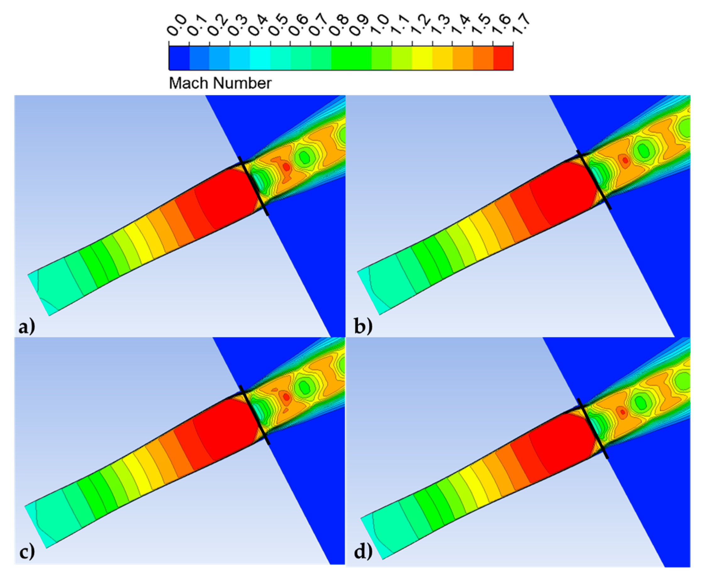
Four CFD simulations were performed, keeping constant the nozzle pressure ratio close to the r2 gas-dynamic condition (shock wave at the nozzle exit): Figure 11 shows Mach number contours for the different working conditions.

Comparing the results to those related to the discharge pressure (p_s) sensitivity analysis, it is evident that operating fluid properties (C_p and MW) have a lower influence on the flow structure and on the Mach number values inside the nozzle.

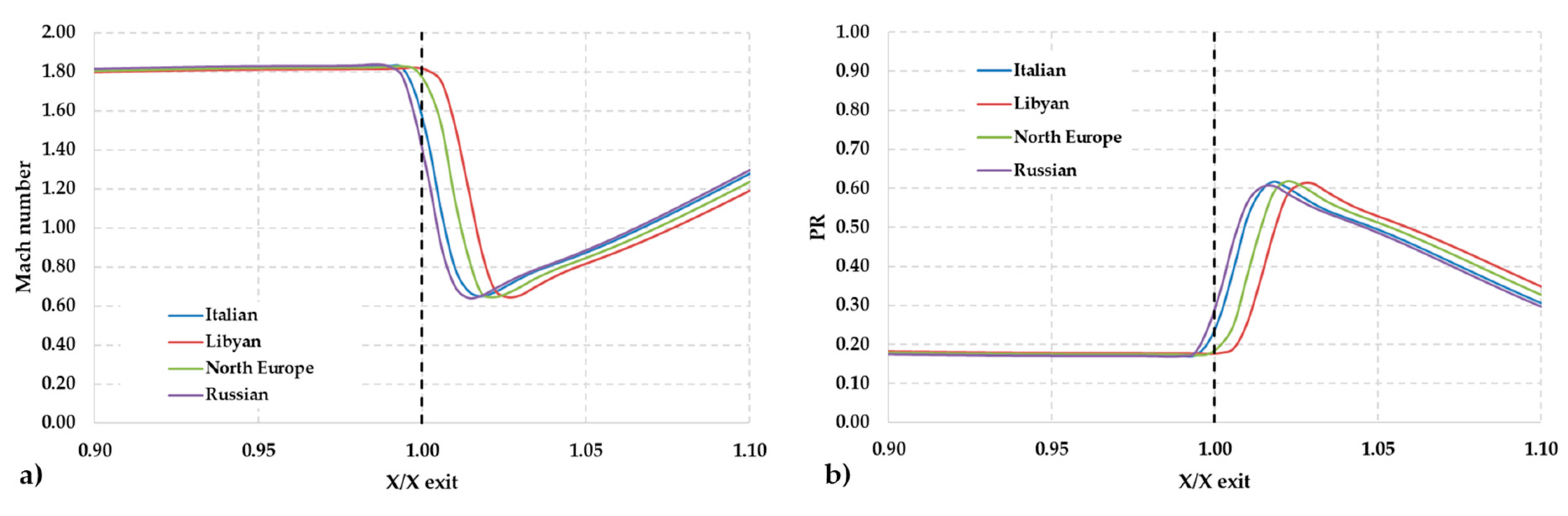
This is also confirmed by the charts in Figure 12, where the Mach number and PR variation along the nozzle axis are displayed. A slight change of the shock wave position can be observed, caused by the different gas properties.

On the other hand, due to gas composition change, a significant variation of the total pressure losses can be noticed (see

Table 8. Total pressure drop values with respect to gas origin.

Natural Gas	Δpt [Pa]
Italian	31,100
Libyan	21,407
North Europe	23,933
Russian	33,579

): more than 10 [kPa] difference within the examined dataset.

4.2. Uncertainty Quantification Analysis

The UQ analysis for the gas composition was performed with the same approach of the previous test. The operating range for the variables C_p and MW (domain space) was identified from the preliminary sensitivity analysis: the specific heat at constant pressure varies from 2031 [J/(kgK)] to 2214 [J/(kgK)], whereas the MW is in the range 16.1 ÷ 19.5 [kg/kmol]. The considered QoI are again the nozzle exit Mach number (M_exit) and the total pressure drop (Δp_t—Equation (3)).

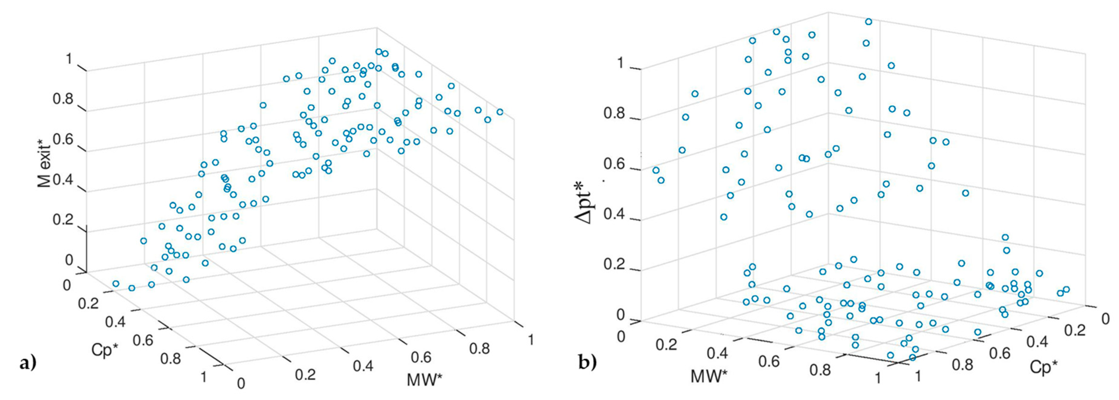
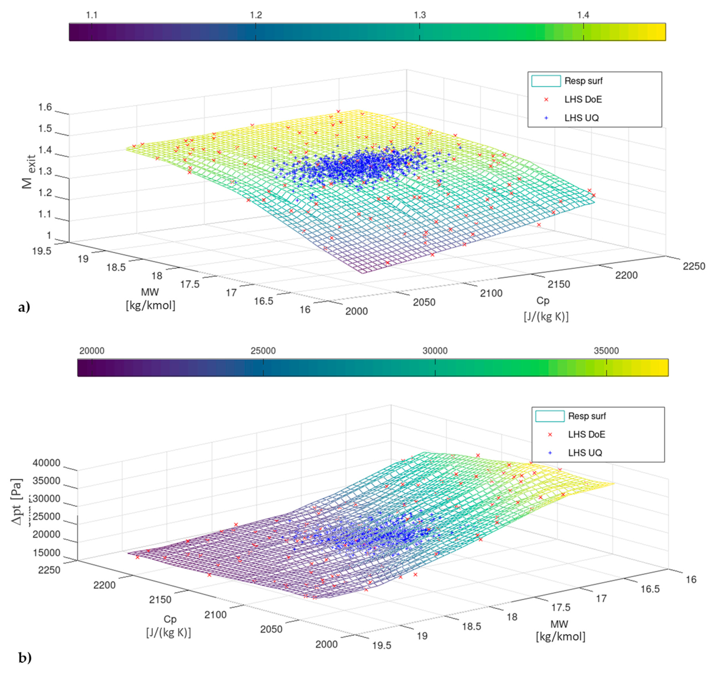
The DoE was generated with 121 samples according LHS methodology. The response functions scattered distributions are reported in Figure 13 (MW* and Cp* are in normalized form, as in Equations (7) and (8)).

$$M{W}^{\ast }=\frac{MW-{\mathrm{MW}}_{\min }}{{\mathrm{MW}}_{\max }-{\mathrm{MW}}_{\min }}$$

(7)

$$C{p}^{\ast }=\frac{Cp-{\mathrm{Cp}}_{\min }}{{\mathrm{Cp}}_{\max }-{\mathrm{Cp}}_{\min }}$$

(8)

A surrogate model based on the DoE (121 samples) was obtained using Kriging Response Surface Methodology. The resulting response surfaces for the QoI are shown in Figure 14.

The cross-validation results reported in

Table 9. Metrics for cross validation analysis of the response surfaces.

Metrics	Mexit	Δpt [Pa]
Root Mean Squared (RMS)	2.87 × 10−3	384.8
Mean Absolute Value	1.65 × 10−3	251.2
Maximum Value	1.42 × 10−2	1416.6

confirm the model reliability. Even in this second application, the validation with three random points of the database was performed.

The results of the challenge set and the comparison in terms of relative percentage error with respect to the CFD results are reported in

Table 10. Metrics for challenge data.

Metrics	Mexit	Δpt [Pa]
Root Mean Squared (RMS)	1.17 × 10−3	283.7
R squared	0.916084	0.806983
Mean Absolute Value	9.99 × 10−4	192.6
Maximum Value	1.81 × 10−3	483.2

and

Table 11. Relative percentage error between CFD and response surface values for random samples.

Cp [J/(kg K)]	MW [kg/kmol]	Percentage Error Mexit	Percentage Error Δpt
2099	17.53	−0.13%	1.80%
2113	17.95	0.06%	−0.39%
2159	18.01	0.02%	−0.02%

respectively.

The low values of the errors certify the reliability of the response surfaces.

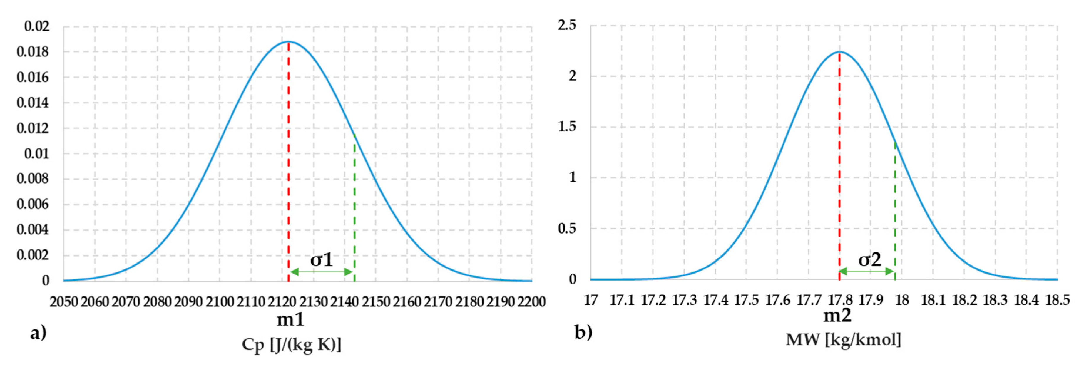
The UQ analysis was implemented according LHS method (1000 samples) in order to evaluate the component response to input variables statistical distributions. A Gaussian probability distribution function was considered for both variables C_p and MW. The characteristics of the pdfs are reported in

Table 12. Pdfs characteristics for the input variables.

Statistical Moments	Cp [J/(kgK)]	MW [kg/kmol]
Mean	2122	17.8
Standard deviation	21.2	0.178

and the corresponding trends are shown in Figure 15.

The mean values m₁ and m₂ of the pdfs were chosen as the arithmetic mean of the selected ranges. The standard deviations σ₁ and σ₂ are about 1% of the corresponding mean values in order to simulate the effects of a small perturbation of the involved variables.

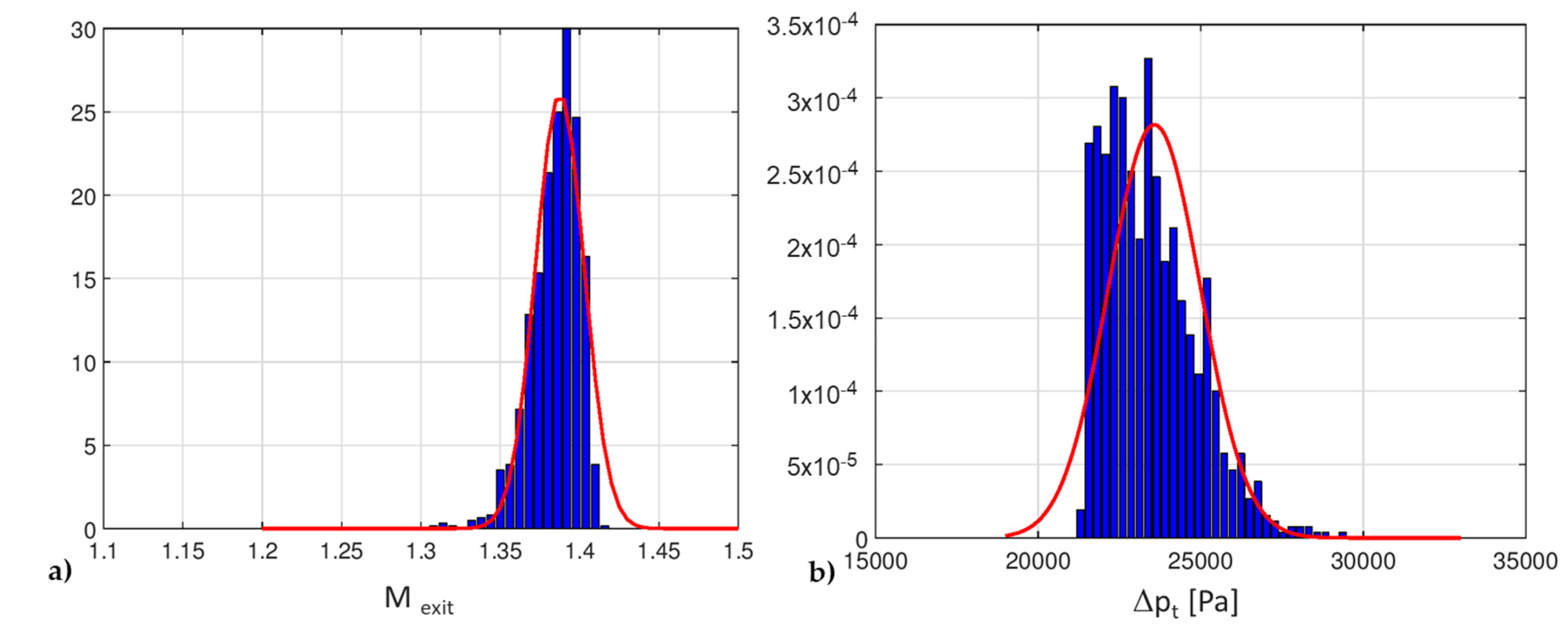
The uncertainties propagation through the meta-model determines the output distributions for the QoI (see Figure 16); the statistical moments of the resulting pdfs are summarized in

Table 13. Statistical moments for the response functions distributions.

Statistical Moments	M exit	Δpt
Mean	1.39	2.36 × 104 [Pa]
Standard Deviation	0.015	1.42 × 103 [Pa]
Skewness	−1.00	0.819
Kurtosis	1.73	0.497

.

The ‘shape’ of the response functions pdfs is very different from the corresponding reference Gaussian distribution: both of them are sharper (positive Kurtosis) and slightly shifted from the mean. The range of M _exit variation, with the selected input, is very narrow. The Mach number is slightly influenced by the gas composition, confirming what was previously observed in the sensitivity analysis.

Regarding total pressure losses, it can be noticed that even with a small variation in Cp and MW, the range of the possible total pressure drop values (Δp_t) is quite wide, and consequently, the probability to fall into a non-optimal operating condition is high.

Finally, to test the results with a higher number of samples, a second UQ analysis was performed with 10,000 LHS samples. The comparison between the statistical distributions of the QoI for the two cases are reported in Figure 17. The very small differences in the pdf trends confirm that 1000 samples are sufficient to accurately detect the system response to input data.

5. Conclusions

The quantitative analysis of the influence on supersonic nozzle performance of the variation of selected input variables leads to the following conclusions.

The perturbation of the discharge pressure ps within a range centered on the r2 operating condition leads to a remarkable variation of the flow structure inside the nozzle, even with a pressure change of a few thousand of Pa, i.e., few percentage points (3% if uncertainty is considered as 3σ) with respect to the r2 discharge pressure condition. This is confirmed by the UQ analysis, with a uniform uncertainty to the input variable (ps), the performance parameters (exit Mach number and total pressure drop) can assume a large range of possible values. If a normal uncertainty is considered, it can be observed that even with a small pressure variation, a significant change in the output parameters is detectable, with a resulting statistical distribution that is very far from the input one, due to the strong non-linearity of the physical problem under study. The investigation on the effects of natural gas composition (C_p, MW) variation showed that it has a slight influence on the flow structure but can remarkably affect the total pressure losses. The UQ analysis with Gaussian uncertainties distributions of the input variables put in evidence a limited effect on the exit Mach number and a non-negligible influence on the total pressure drop that has a wide range of variation. The statistical distributions of the output variables differ from the normal pdfs of the input parameters because of the uncertainties propagation through the nonlinear model. The proposed workflow for the UQ analysis, implemented into the Dakota platform, has shown its effectiveness in a quantitative evaluation of the effect of changes in input parameters on the response functions of the engineering design problem; it may be applied to other design applications with the same structure.

References

- Cravero, C.; Dawes, W.N. Throughflow design using an automatic optimisation strategy. In Proceedings of the ASME Turbo Expo ’97, Orlando, FL, USA, 2–5 June 1997. [Google Scholar]
- Barsi, D.; Costa, C.; Cravero, C.; Ricci, G. Aerodynamic design of a centrifugal compressor stage using an automatic optimization strategy. In Proceedings of the ASME Turbo Expo, Dusseldorf, Germany, 16–20 June 2014. ASME paper GT2014-26465. [Google Scholar]
- Cravero, C.; Macelloni, P.; Briasco, G. Three-dimensional design optimization of multi stage axial flow turbines using a RSM based approach. In Proceedings of the ASME Turbo Expo, Copenhagen, Denmark, 5–11 June 2012. ASME paper GT2012-68040. [Google Scholar]
- Cravero, C. Turbomachinery design optimization based on metamodels. In Proceedings of the 4th Inverse Problems Design and Optimization Symposium IPDO-2013, Albi, France, 26–28 June 2013; ISBN 979-10-91526-01-2. [Google Scholar]
- Campora, U.; Capelli, M.; Cravero, C.; Zaccone, R. Metamodels of a Gas Turbine Powered Marine Propulsion system for Simulation and Diagnostic Purposes. J. Nav. Arch. Mar. Eng. 2015, 12, 1–14. [Google Scholar] [CrossRef] [Green Version]
- Campora, U.; Cravero, C.; Zaccone, R. Marine Gas Turbine Monitoring and Diagnostics by Simulation and Pattern Recognition. Int. J. Nav. Arch. Ocean Eng. 2018, 10, 617–628. [Google Scholar] [CrossRef]
- Anderlini, A.; Salvetti, M.V.; Agresta, A.; Matteucci, L. Stochastic sensitivity analysis of numerical simulations of injector internal flows to cavitation modeling parameters. Comput. Fluids 2019, 183, 130–147. [Google Scholar] [CrossRef]
- Anderson, J.D. Modern Compressible Flow, 2nd ed.; McGraw Hill: New York, NY, USA, 1990; pp. 147–179. [Google Scholar]
- Laws, C.J. A Simple Method for the Design of Gas Burners Injectors. Proc. Inst. Mech. Eng. PartC-J. Mech. Eng. Sci. 2003, 217, 237–246. [Google Scholar]
- Ogawa, H.; Boyce, R.R.; Isaacs, A.; Ray, T. Multi-Objective Design Optimisation of Inlet and Combustor for Axisymmetric Scramjets. Open Thermodyn. J. 2010, 4, 86–91. [Google Scholar] [CrossRef]
- Karimi, A.; Abdi, M.A. Selective Dehydration of high-pressure natural gas using supersonic nozzles. Chem. Eng. Process. Process. Intensif. 2009, 48, 560–568. [Google Scholar] [CrossRef] [Green Version]
- Yang, Y.; Li, A.; Wen, C. Optimization of static vanes in a supersonic separator for gas purification. Fuel Process. Technol. 2017, 156, 265–270. [Google Scholar] [CrossRef]
- Montomoli, F.; Carnevale, M.; D’Ammaro, A.; Massini, M.; Salvadori, S. Uncertainty Quantification in Computational Fluid Dynamics and Aircraft Engines; Springer: Berlin, Germany, 2015; pp. 59–84. [Google Scholar]
- Adams, B.M.; Bohnhoff, W.J.; Dalbey, K.R.; Eddy, J.P.; Ebeida, M.S.; Eldred, M.S.; Frye, J.R.; Gerarci, G.; Hooper, R.W.; Hough, P.D.; et al. Dakota, a Multilevel Parallel Object-Oriented Framework for Design Optimization, Parameter Estimation, Uncertainty Quantification and Sensitivity Analysis. Version 6.11 User’s Manual; Sandia National Laboratories: Albuquerque, NM, USA, 2019. [Google Scholar]
- Helton, J.C.; Davis, F.J. Latin hypercube sampling and the propagation of uncertainty in analyses complex systems. Reliab. Eng. Syst. Saf. 2003, 81, 23–69. [Google Scholar] [CrossRef] [Green Version]
- Helton, J.C.; Johnson, J.D.; Sallaberry, C.J.; Storlie, C.B. Survey of sampling-based methods for uncertainty and sensitivity analysis. Reliab. Eng. Syst. Saf. 2006, 91, 1175–1209. [Google Scholar] [CrossRef] [Green Version]
- McKay, M.D.; Beckman, R.J.; Conover, W.J. A Comparison of Three Methods for Selecting Values of Input Variables in the Analysis of Output from a Computer Code. Technometrics 1979, 21, 239. [Google Scholar] [CrossRef]
- Available online: https://misura.snam.it/portmis/coortecDocumentoController.do?menuSelected=4300 (accessed on 20 January 2020).
- Basso, D.; Cravero, C.; Reverberi, A.P.; Fabiano, B. CFD Analysis of Regenerative Chambers for Energy Efficiency Improvement in Glass Production Plants. Energies 2015, 8, 8945–8961. [Google Scholar] [CrossRef] [Green Version]
- Arnulfi, G.L.; Cravero, C.; Marini, M. Analysis of the operating mode influence onto Energy consumption of a natural gas storage plant. In Proceedings of the ASME Turbo Expo, Copenhagen, Denmark, 11–15 June 2012. [Google Scholar]
- Shishmi, E.; Ben-Dor, G.; Levy, A. Viscous simulation of shock-reflection hysteresis in overexpanded planar nozzles. J. Fluid Mech. 2009, 635, 189. [Google Scholar] [CrossRef]
- Zapryagaev, V.I.; Kudryavtsev, A.N.; Lokotko, A.V.; Solotchin, A.V.; Pavlov, A.A.; Hadjadj, A. An Experimental and Numerical Study Of A Supersonic-Jet Shock-Wave Structure. In Proceedings of the 11th International Conference on Methods of Aerophysical Research, Novosibirsk, Russia, 1–7 July 2002. [Google Scholar]
Figure 1.
Fluid domain.
Figure 2.
Nozzle mesh.
Figure 3.
Mach number contours for five ps values: (a) 80 kPa, (b) 90 kPa, (c) 100 kPa, (d) 110 kPa, (e) 120 kPa; the black line identifies nozzle exit section.
Figure 4.
(a) Mach number and (b) PR along nozzle axis.
Figure 5.
Response functions: (a) Mach number at nozzle exit, (b) Nozzle total pressure drop.
Figure 6.
Histograms of the pdf for the output functions: (a) Mexit, (b) Δpt.
Figure 7.
Comparison between 1000 and 10,000 samples for the sampling-based UQ analysis. Probability density functions for: (a) M exit; (b) Δpt.
Figure 8.
Normal pdf of the input discharge pressure ps.
Figure 9.
Histograms of the pdfs for the output functions: (a) M exit, (b) Δpt; the red curves represent the corresponding Gaussian normal distributions.
Figure 10.
Figure 11.
Mach number contours: (a) Italian, (b) Libyan, (c) North Europe, (d) Russian.
Figure 12.
(a) Mach number and (b) PR along the nozzle axis.
Figure 13.
DoE: (a) Mach number at nozzle exit, (b) Total pressure losses.
Figure 14.
Response surfaces obtained from the DoE for (a) Mexit (b) Δpt.
Figure 15.
Gaussian pdfs of the input variables.
Figure 16.
Histograms of the pdf for the output functions: (a) M exit, (b) Δpt; red curves represent the corresponding normal distributions.
Figure 17.