Improved Convergence Speed of a DCD-Based Algorithm for Sparse Solutions


School of Information Engineering, Zhengzhou University, Zhengzhou 450001, China
*
Author to whom correspondence should be addressed.
Algorithms 2020, 13(6), 136; https://0-doi-org.brum.beds.ac.uk/10.3390/a13060136
Submission received: 6 May 2020
/
Revised: 22 May 2020
/
Accepted: 26 May 2020
/
Published: 4 June 2020
Abstract
:To solve a system of equations that needs few updates, such as sparse systems, the leading dichotomous coordinate descent (DCD) algorithm is better than the cyclic DCD algorithm because of its fast speed of convergence. In the case of sparse systems requiring a large number of updates, the cyclic DCD algorithm converges faster and has a lower error level than the leading DCD algorithm. However, the leading DCD algorithm has a faster convergence speed in the initial updates. In this paper, we propose a combination of leading and cyclic DCD iterations, the leading-cyclic DCD algorithm, to improve the convergence speed of the cyclic DCD algorithm. The proposed algorithm involves two steps. First, by properly selecting the number of updates of the solution vector used in the leading DCD algorithm, a solution is obtained from the leading DCD algorithm. Second, taking the output of the leading DCD algorithm as the initial values, an improved soft output is generated by the cyclic DCD algorithm with a large number of iterations. Numerical results demonstrate that when the solution sparsity is in the interval , the proposed leading-cyclic DCD algorithm outperforms both the existing cyclic and leading DCD algorithms for all iterations.
1. Introduction
With the development of information technology, the number of participated devices and data transmission rate have substantially increased in recent years. Solving the problems in a wide range of signal processing applications is equivalent to getting the solution of a linear least squares (LS) problem [1]. These applications include adaptive antenna array applications [2], multi-user detection [3], multiple-input multiple-output (MIMO) detection [4], echo cancellation [5], equalization [6], and system identification [1,7,8,9]. If the channel information is known, zero forcing (ZF) algorithm and minimum mean-square error (MMSE) algorithm are popular to be used in these applications. They are simple to implement but require the operation of matrix inversion.
The complexity of matrix inversion requires arithmetic operations, where U is system size [10]. When the system size is large, the complexity of the matrix inversion is prohibitively high. As a result, there are some techniques proposed to solve systems of equations without inverting the matrix. Direct methods, for example Gaussian elimination, Cholesky factorization, and QR decomposition attain a complexity of [10,11]. Therefore, it is difficult for direct methods to be implemented in real-time signal processing and hardware applications. Using these methods to solve the linear equations of large sparse systems may be prohibitively expensive and are infeasible for practical applications. Iterative methods, for example, the conjugate gradient method and the steepest descent method could achieve fast convergence. In each iteration, they require complexity. Other iterative methods, for example, the Southwell’s relaxation [12], Jacobi [10] and Gauss-Seidel [10], are coordinate descent approaches. At each iteration, they only require complexity but have a slower convergence speed. The number of iterations performed decides the computational complexity of these techniques. Iterative methods can solve problems with sparse structures more efficiently compared with direct methods [13]. Moreover, iterative methods have the potential to achieve a good initial guess for the expected results, which can reduce the number of iterations required to obtain a solution [14]. However, some iterative methods include the numerical operations of multiplying or dividing, which are difficult for hardware implementation.
Prior research work investigates the dichotomous coordinate descent (DCD) algorithms that use a reduced number of operations to solve systems of equations. DCD-based algorithms are well known in many applications because the DCD algorithm avoids the operations of multiplying and dividing, which are expensive to implement. In [15,16,17], by applying the DCD iterations, the numerical complexity of affine projection algorithms for active noise control is reduced. In [18], DCD iterations solve the recursive least squares (RLS) matrix inversion problem by using bit-shift. The DCD algorithm [14,19] is a non-stationary iterative method based on stationary CD techniques. Only additions or additions are required in each iteration [11]. The DCD algorithm, therefore, is a good choice for real-time hardware implementations. The DCD algorithm variants, cyclic DCD and leading DCD algorithm, were presented in [20]. When scenarios with sparse true solutions are considered, such as multi-path channel estimation and detection of a multi-user system with several unknown active users, the leading DCD algorithm converges faster than the cyclic DCD algorithm. The cyclic DCD algorithm is ideal for solving systems of equations that require a large number of iterations because it converges faster and has a lower error level than the leading DCD algorithm. However, the leading DCD algorithm has a faster convergence rate than the cyclic DCD algorithm in the initial iterations if the solution is not very sparse.
In this paper, we considered a combination of leading and cyclic DCD iterations and proposed a leading-cyclic DCD algorithm for obtaining a sparse solution in systems requiring a large number of updates. The idea is that the leading DCD algorithm uses a small number of iterations to obtain the initial input for the cyclic DCD algorithm. The number of iterations used in the leading DCD algorithm has been thoroughly investigated under different system matrix conditions and solution sparsities. In the proposed algorithm, a range of the number of iterations is determined that will produce an optimal number of updates for the leading DCD algorithm. The results show that the proposed leading-cyclic DCD algorithm improves the convergence speed of the cyclic DCD algorithm and lowers the steady-state level.
Notation: Boldface uppercase and boldface lowercase letters represent matrices and vectors (e.g., and ). Elements of matrix and vector are denoted as and , respectively. The n-th column of is denoted as . denotes a matrix transpose, and denotes the Hermitian transpose.
2. Preliminaries
We start by introducing the system model used in this work. We then discuss the DCD algorithms used to solve the linear model.
2.1. System Model
The system linear model can be modeled as
where is a matrix, is a received vector, and is a unknown vector. We assume that and the matrix and vectors are real-valued. In addition, K () elements of vector are non-zero. For example, is a sparse vector, and the index set of non-zero values is not given. There are many applications to solve problems with sparse true solutions. The multi-path communication channels, concerning the uncertainty delay interval, several multi-path components can be very small. The maximum likelihood (ML) estimation is usually applied to solve normal equations [21], to achieve the sparse true solutions in sparse multi-path channels. Multi-user detection can be considered to be another example when the number of active users K is less than the expected number of users U [22]. Whether the matrix can be pre-computed determines the different computational complexity of sparse solution estimators. Calculation of the matrix is complex for the algorithm. The pre-computed matrix leads to the low complexity of the algorithm. In this work, we assume that matrix is known. The vector of the signal is calculated as:
where . It costs complexity for computing the matrix inversion directly. The matrix inversion computing becomes prohibitively high when the system size U increases. To avoid such a high computational complexity, we can solve the normal Equation (1) by minimizing the quadratic function:
To solve (3), an iterative descent search method can be applied as a possible choice. The descent search method updates the solution vector via at each iteration i, where is the update direction of the solution. The direction is designed to be non-orthogonal to the residual vector (). When current is not the exact point, i.e., , it shows that the descent search method converges to the original problem solution with descent objective values in the convex area.
2.2. DCD Algorithms
The DCD algorithm is one of many iterative techniques for solving the linear LS problem [19]. There are bits to represent the elements of the solution vector. The amplitude of the element is limited to . The iterative search begins with the most significant bits of the solution and ends with the least significant bits updated. The execution is controlled by the step size (). starts at and decreases as for less significant bits. DCD-based techniques usually use bit-shift to replace the multiplication/division operations, which is attractive for hardware implementation. The variants of the DCD algorithm: cyclic DCD algorithm and leading DCD algorithm, have different properties and been applied to different applications. These algorithms are described below.
2.2.1. Cyclic DCD Algorithm
The cyclic DCD algorithm [20], which is described in Table 1, updates a solution vector in cyclic order (). In each iteration, when an element of the solution vector is updated, we call it a “successful” update. When updates, the algorithm executes the successful updates until the elements in the residual vector are too small to meet the condition in step 3. Then, is updated in step 1. The number of successful iterations p and the number of bits are the essential parameters of the algorithm. They determine the main computational complexity of the cyclic DCD algorithm. The maximum number of successful iterations, , is predetermined. It can be used as a stopping condition for the algorithm. For a given and , the computational complexity of the cyclic DCD algorithm is restricted to an upper limit additions. However, the cyclic order update is not an efficient choice for solving a system of equations that needs a few updates.
2.2.2. Leading DCD Algorithm
A good method of index selection may speed up the convergence. The leading DCD algorithm [20] is briefly described in Table 2. The index n in the leading DCD algorithm is chosen via . The (n-th) element in corresponds to the (n-th) element in the residual vector that has the largest absolute value. Given several iterations , the computational complexity of the leading DCD algorithm is restricted to an upper limit additions.
2.2.3. Complexity Discussion
Table 1 shows that when is much larger than , then the computational complexity of the cyclic DCD is dominated by additions. When the value is small, then the computational complexity is upper bounded by the term .
2.2.4. Numerical Results
In this section, numerical results show that cyclic and leading DCD algorithms deal with system matrices with different condition numbers. We consider real-valued systems here. The condition number of the matrix is attained by modifying the ratio between Q and U. Usually when U is closer to Q, the matrix condition number is higher. For example, performing a highly loaded multi-user detection is equivalent to solving a linear equation , where is the output vector of the matched filter. is a randomly generated transmitted data vector whose elements are uniformly distributed on .
Using the DCD algorithm to solve (1), an estimated solution is obtained. We determine the misalignment between and as
The misalignments are averaged by 100 simulation trials and plotted (in decibels) against the number of updates.
Figure 1 depicts the misalignments of the cyclic and leading DCD algorithms. A system matrix is designed with small condition numbers in the interval . It is seen that the cyclic DCD algorithm has a slightly slower convergence than the leading DCD algorithm.
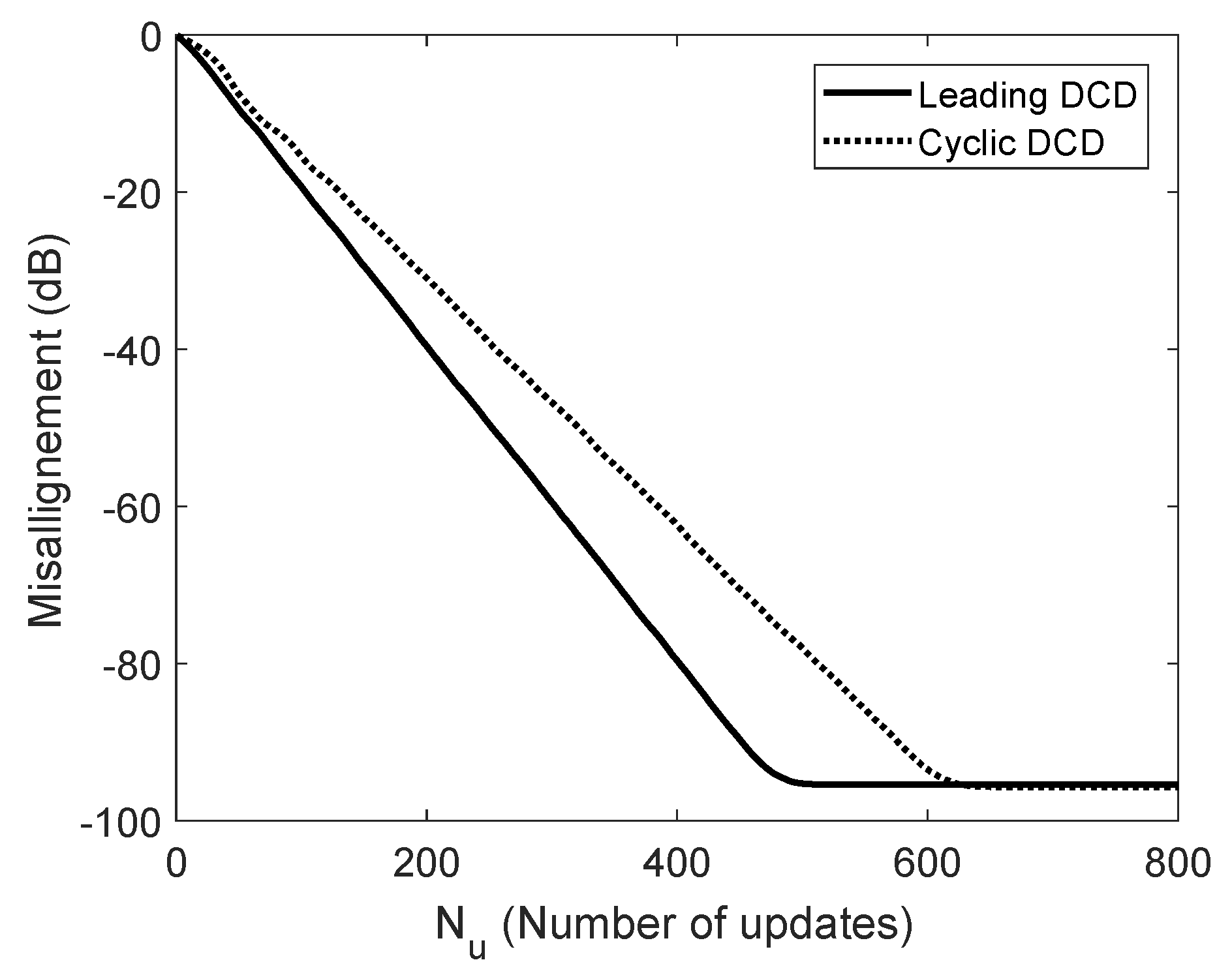
Figure 2 depicts the misalignments of the cyclic and leading DCD algorithms in the system with high condition numbers in the range of . It shows that the cyclic DCD algorithm has a faster convergence than the leading DCD algorithm. Also, the convergence speed of the two DCD algorithms is slower than that in Figure 1.
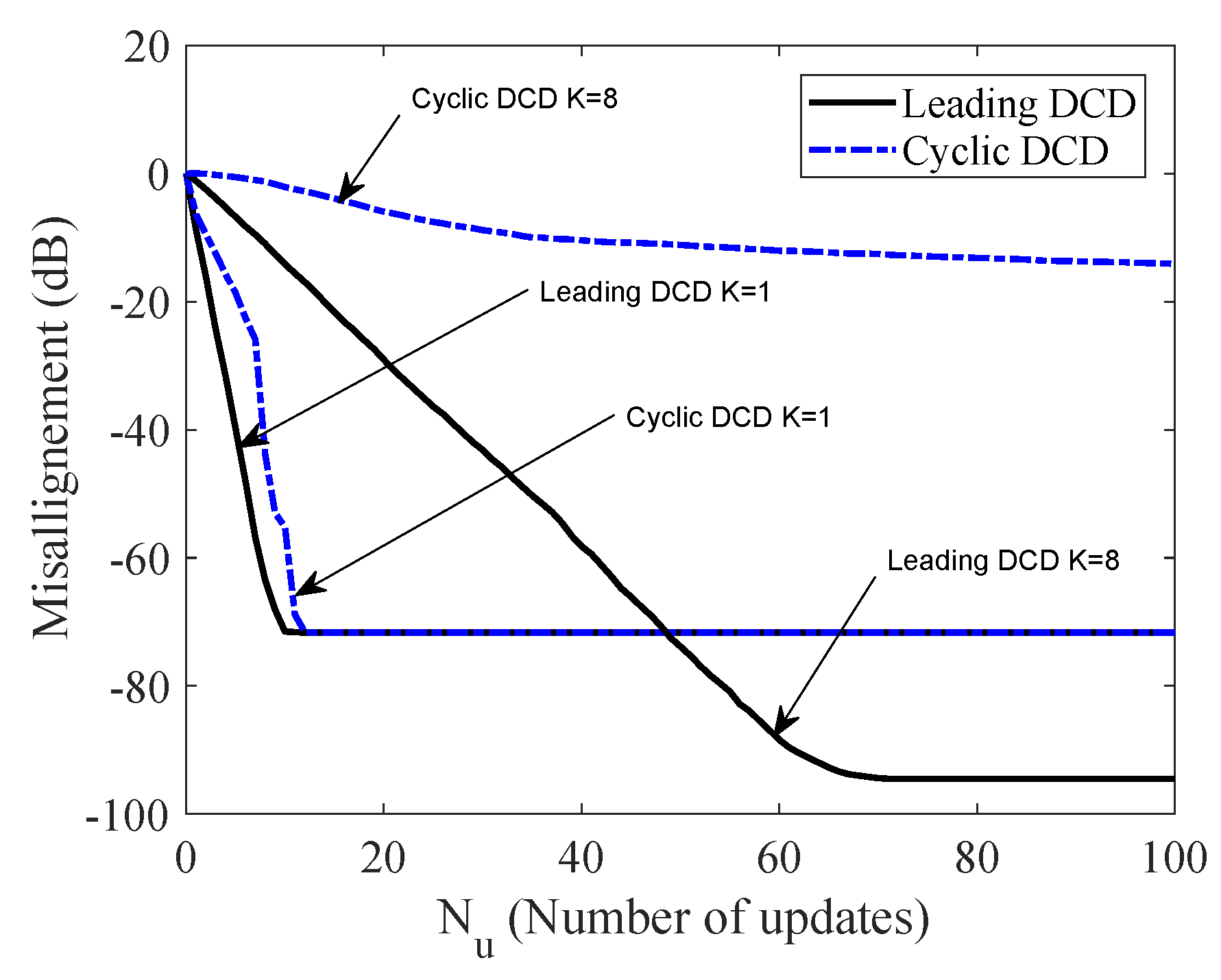
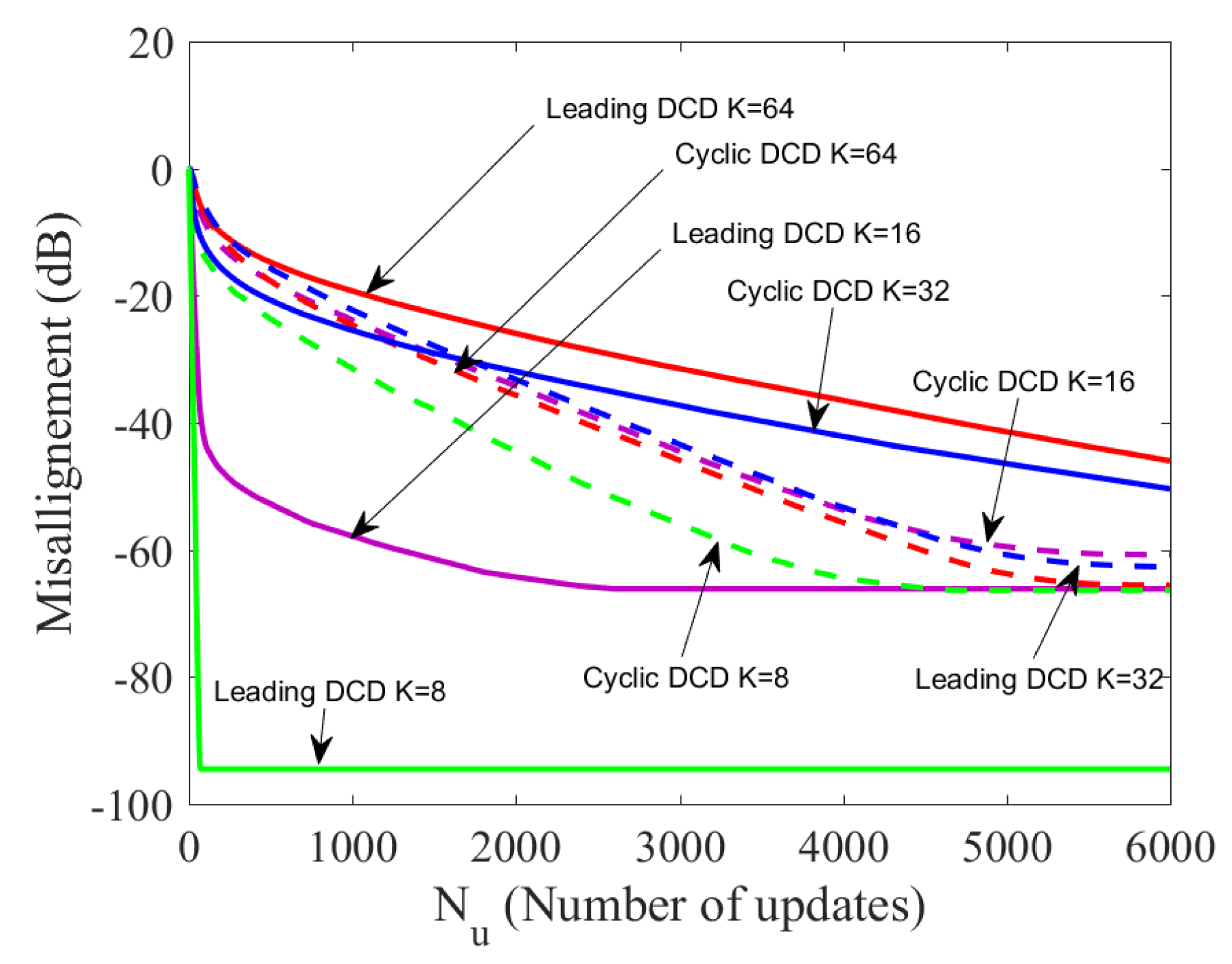
When we consider a scenario with a sparse true solution, the number of updates is expected to be reduced. Figure 3 and Figure 4 display misalignments of the DCD algorithms in the case of a system matrix with high condition numbers. It is seen that the solution is sparser, the convergence of the DCD algorithm is faster.
From the results in Figure 3 and Figure 4, we can see that in the case of , compared to the non-sparse system, the number of iterations required by the leading DCD algorithm to attain a misalignment of dB is approximately reduced by a factor of 20. However, for the cyclic DCD algorithm, the number of iterations reduction is not significant. The number of updates required in the leading DCD algorithm is approximately reduced by a factor of 30 in the case of . For the cyclic DCD algorithm, the number of iterations is approximately reduced by a factor of . Therefore, the leading DCD algorithm is preferable for highly sparse scenarios because it could achieve a significant reduction in the number of updates. When , we can see that the cyclic DCD algorithm has a lower steady-state misalignment; however, the leading DCD algorithm has a faster convergence speed in the initial iterations. When (non-sparse system), the cyclic DCD algorithm has faster convergence and lower steady-state misalignment than the leading DCD algorithm.
3. Proposed Leading-Cyclic DCD Algorithm
From the results above, we can see that the cyclic DCD algorithm is more suitable for solving a non-sparse system with a large condition number. However, it is noted that when the percentage of non-zero elements of the solution is approximately , the leading DCD algorithm provides a faster convergence in the initial updates. To further improve the convergence when the solution is not highly sparse, we consider combining the leading and cyclic DCD algorithms and propose the leading-cyclic DCD algorithm shown in Table 3.
The proposed algorithm involves two steps. In the first step, a data vector is obtained using the leading DCD algorithm with a considerably smaller number of iterations than in the standard version of the leading DCD algorithm. In the second step, an improved soft output is generated by applying the cyclic DCD algorithm with a large number of iterations . The updated vectors of and and the step size of obtained from the leading DCD algorithm are the initial values for the cyclic DCD algorithm. There are two factors that determine the worst-case computational complexity of the leading-cyclic DCD algorithm. The cyclic DCD algorithm starts at bit for updating an element of the solution. The upper computational complexity of the cyclic DCD algorithm is calculated as follows. For the m-th bit, has successful iterations. That is, executing the initial bits does not include a successful iteration and thus requires additions. Among the U iterations , if there is only one successful iteration, then calculating the last bit requires U additions for the comparison and additions for updating the residual vector and elements . In total, successful iterations require additions. The upper bound of computational complexity of the cyclic DCD algorithm is additions. The worst-case scenario for the complexity of the leading DCD algorithm occurs when the algorithm uses all updates. By using iterations, the computational complexity of the leading DCD algorithm is additions. Therefore, the computational complexity of the leading-cyclic DCD algorithm has an upper limit of real-valued additions. In a practical situation, in each pass there should be several successful updates, and the average complexity is close to . is approximately equal to ; therefore, the average complexity of the leading-cyclic DCD algorithm is close to that of the cyclic DCD algorithm.
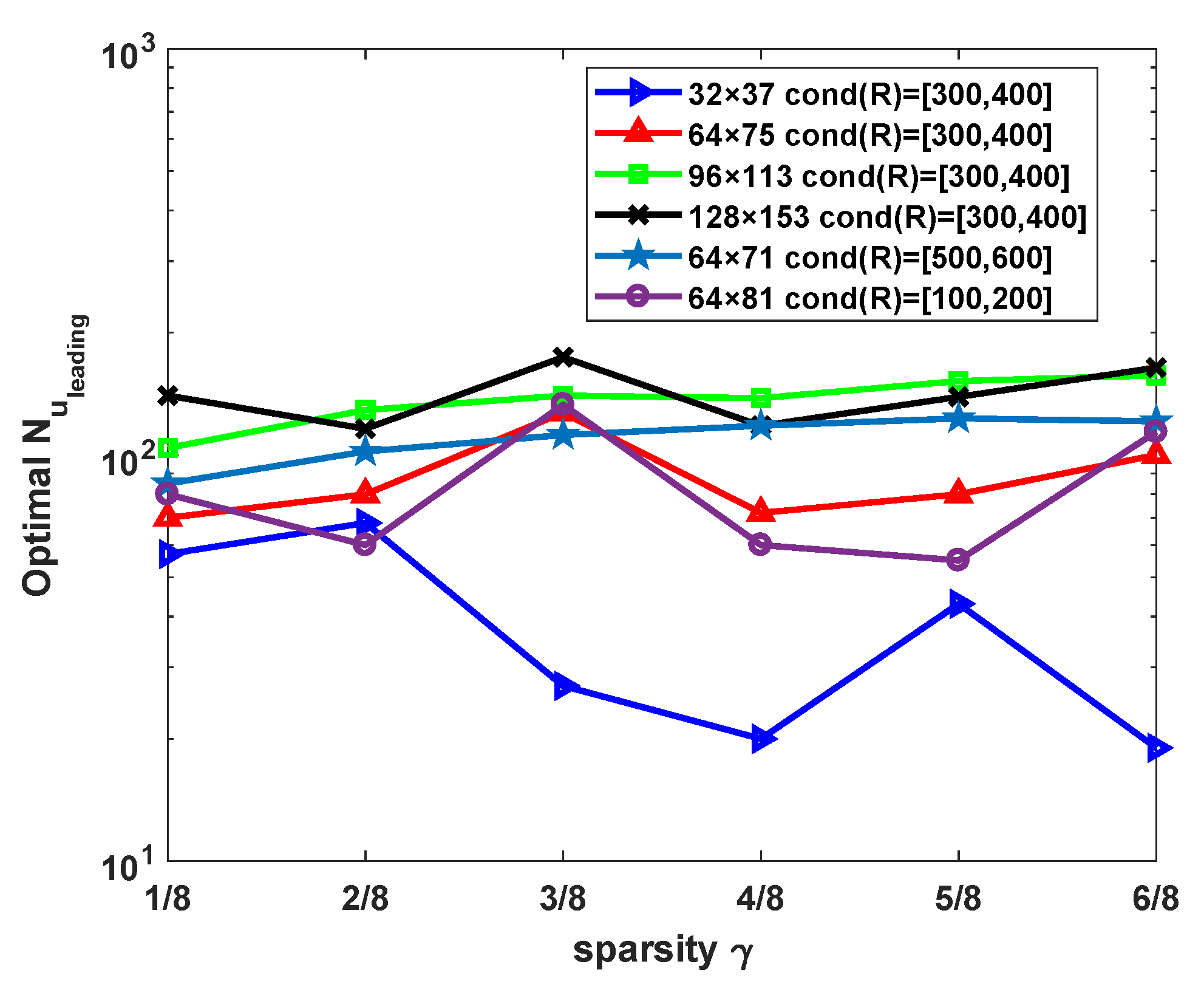
The selection of varies based on the system matrix condition and the solution sparsity. The leading-cyclic algorithm is evaluated by using different values in the range of . Among these values of , the one that allows the proposed algorithm to achieve the fastest convergence to the steady-state level is chosen as the optimal . Figure 5 shows the optimal in the leading-cyclic DCD algorithm for matrices with different sparsities .
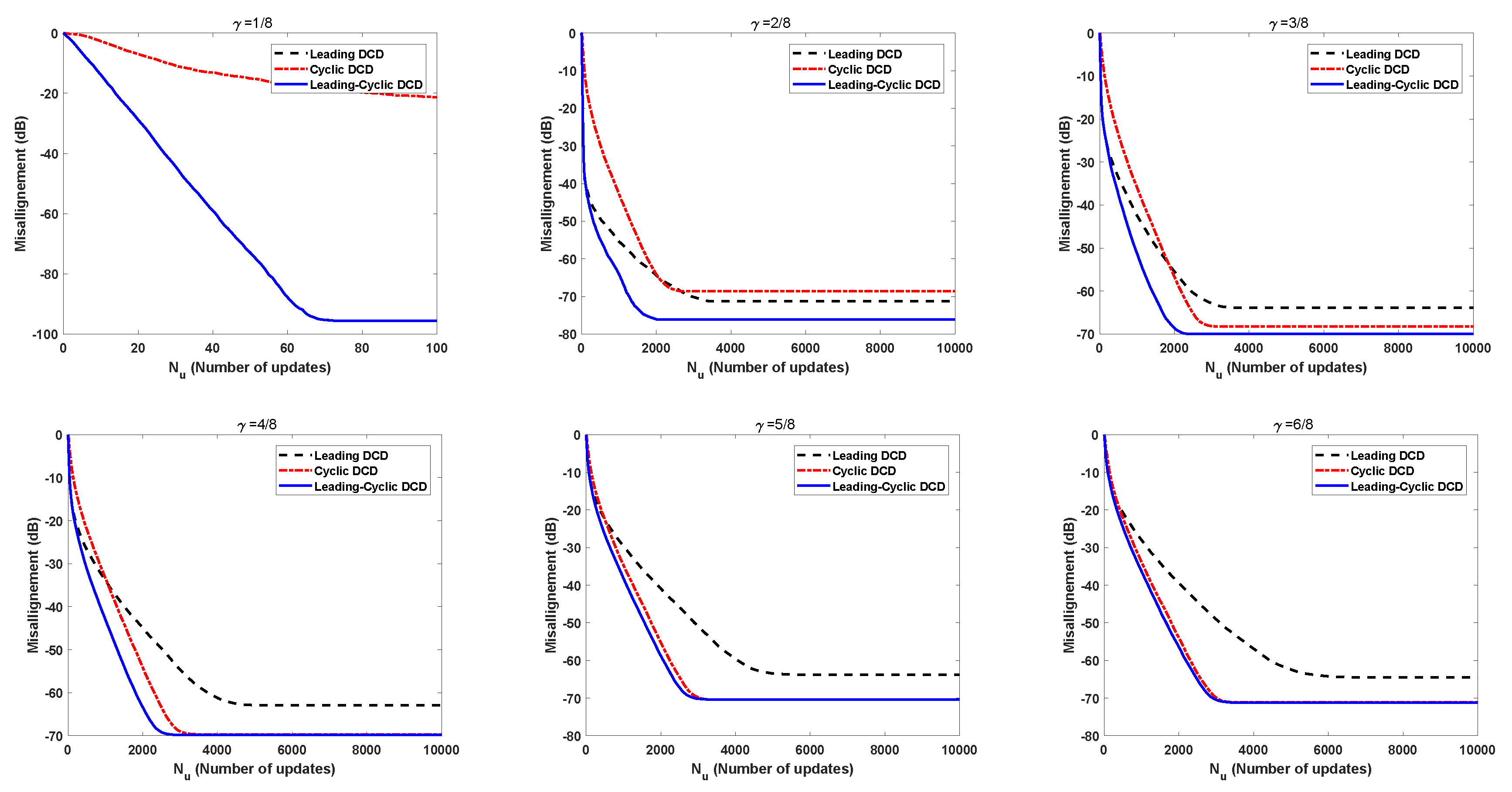
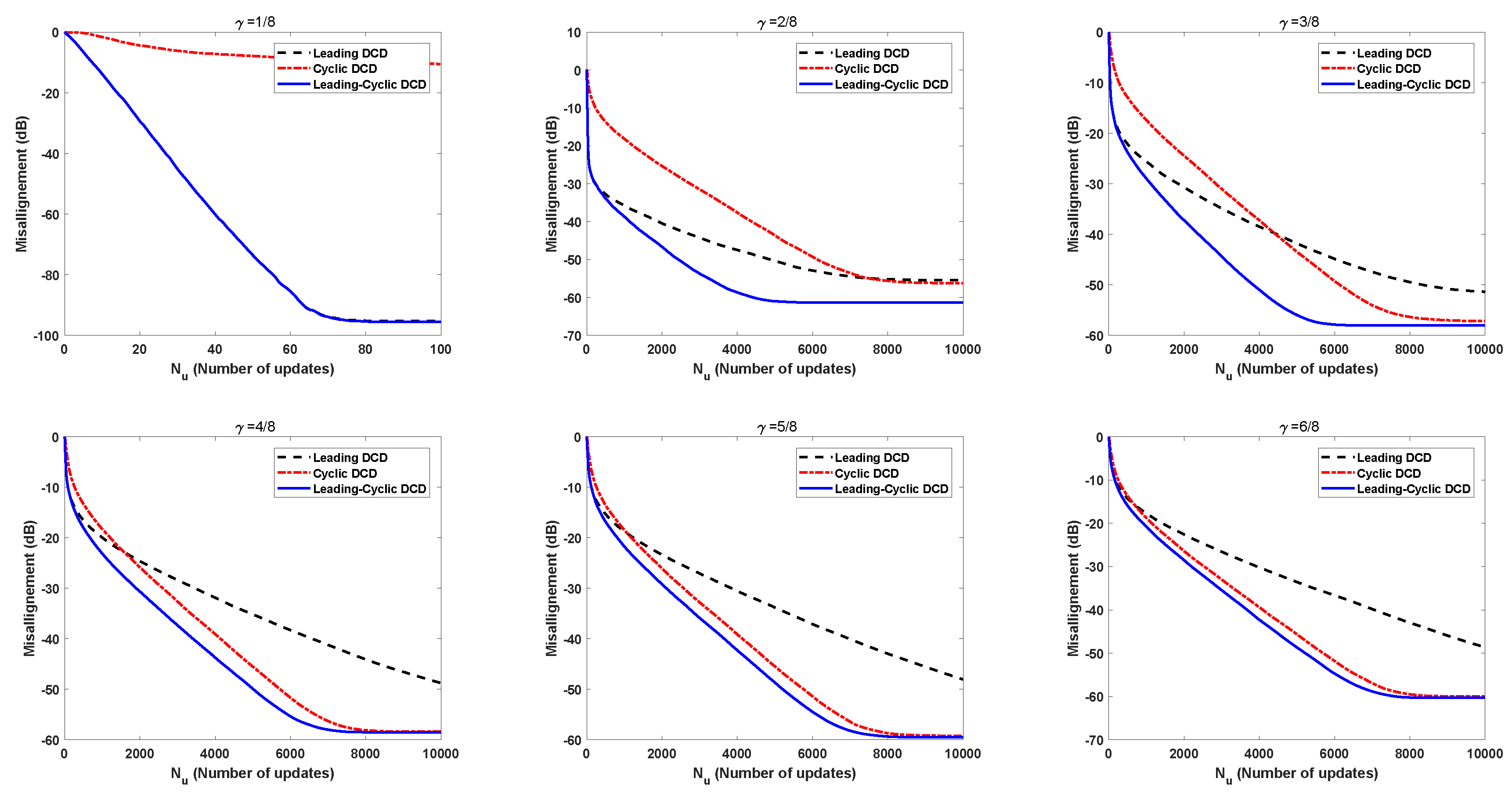
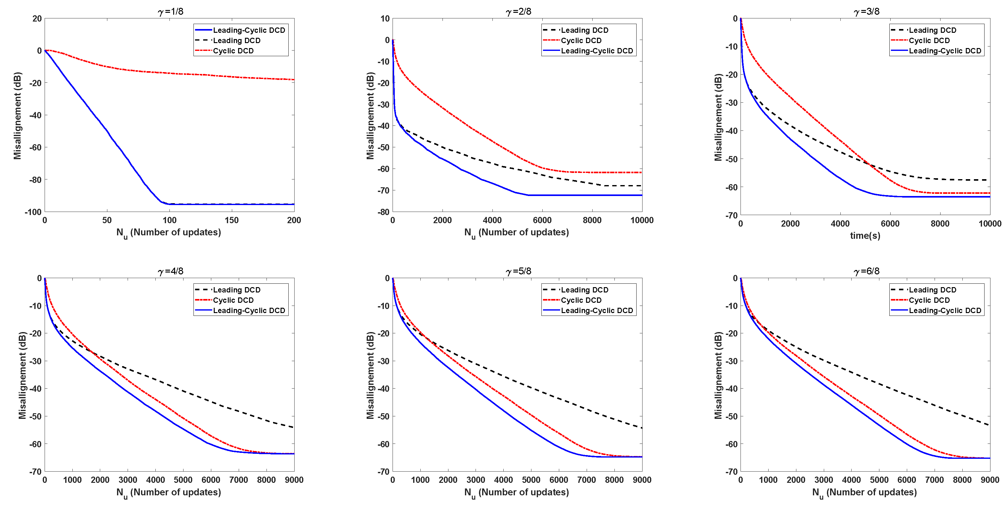
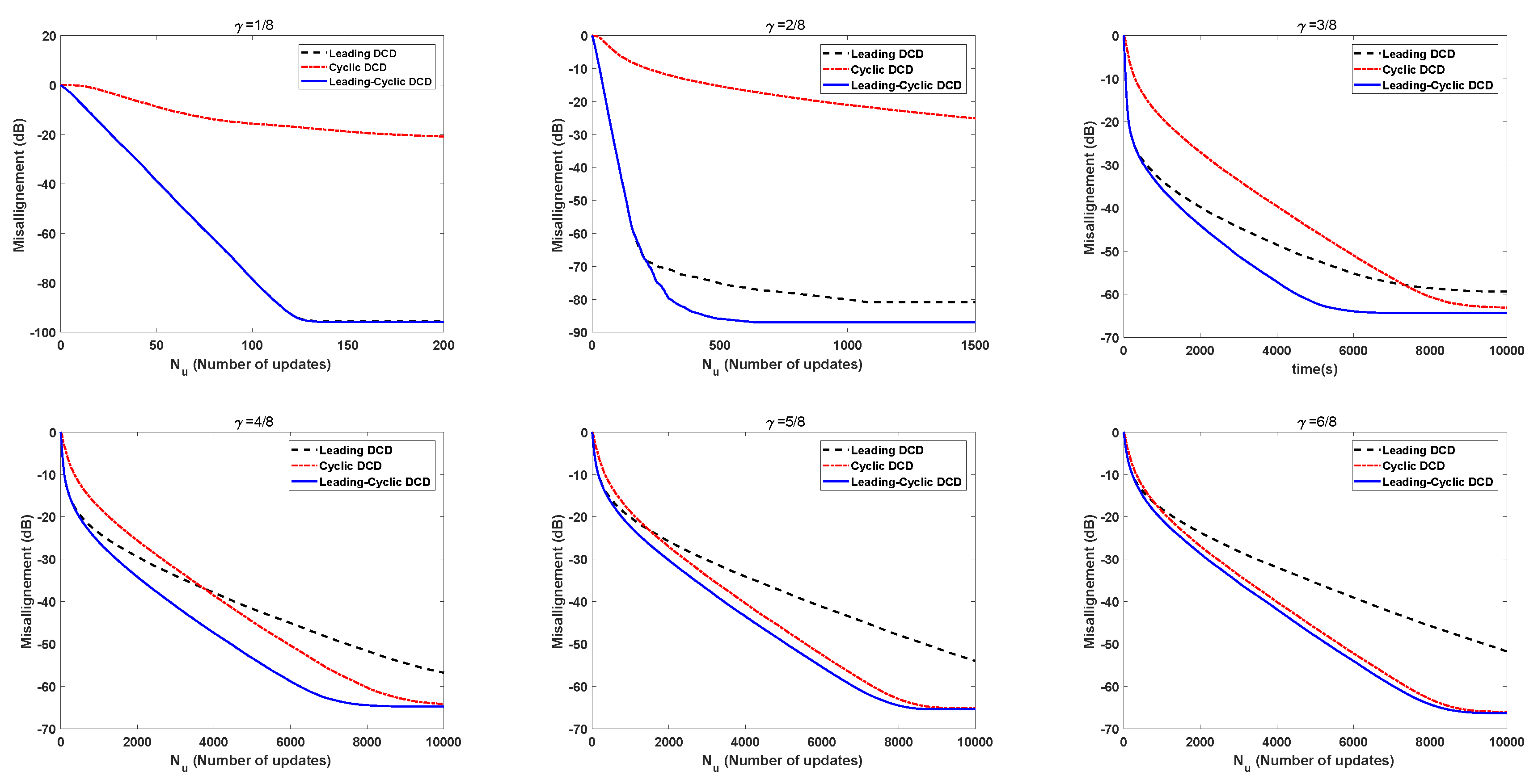
The misalignments compared to the number of successful iterations for large system matrices with condition numbers (≥100) and sparse solutions are shown in Figure 6, Figure 7, Figure 8, Figure 9, Figure 10 and Figure 11. By comparing the results from Figure 6 and Figure 7, we can see that the lower the condition number of the system matrix is, the faster the convergence speed and the lower the steady-state level of these DCD algorithms. From these figures, we can see that when , the leading DCD algorithm has a significantly faster convergence speed and a lower steady-state misalignment than the cyclic DCD algorithm. The leading-cyclic DCD algorithm has approximately the same steady-state level as the leading DCD algorithm. As increases, the cyclic DCD algorithm gradually outperforms the leading DCD algorithm. The leading-cyclic DCD algorithm with a given (shown in Figure 5) has an increased convergence speed and a lower steady-state misalignment compared to the leading DCD algorithm. When increases to , the leading-cyclic DCD algorithm exhibits an insignificantly increased convergence speed compared to the cyclic DCD algorithm.
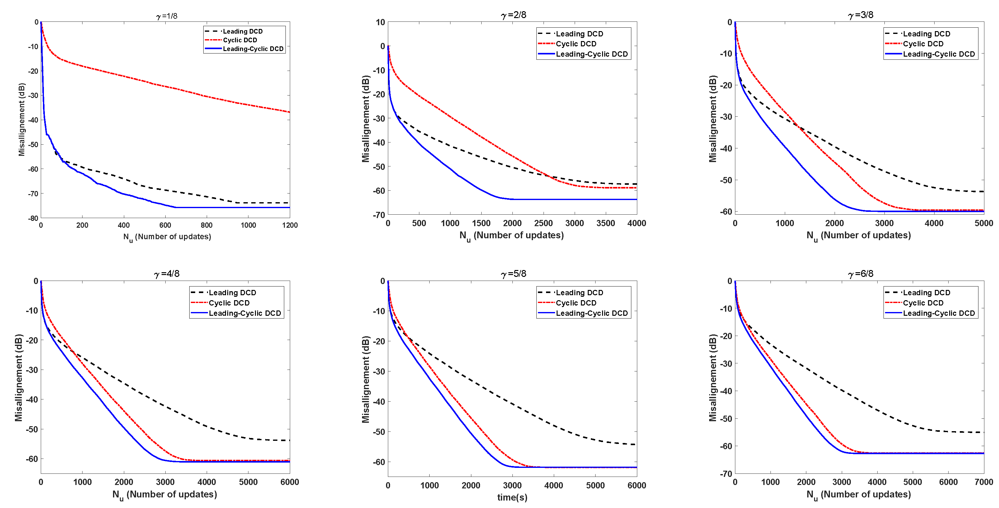
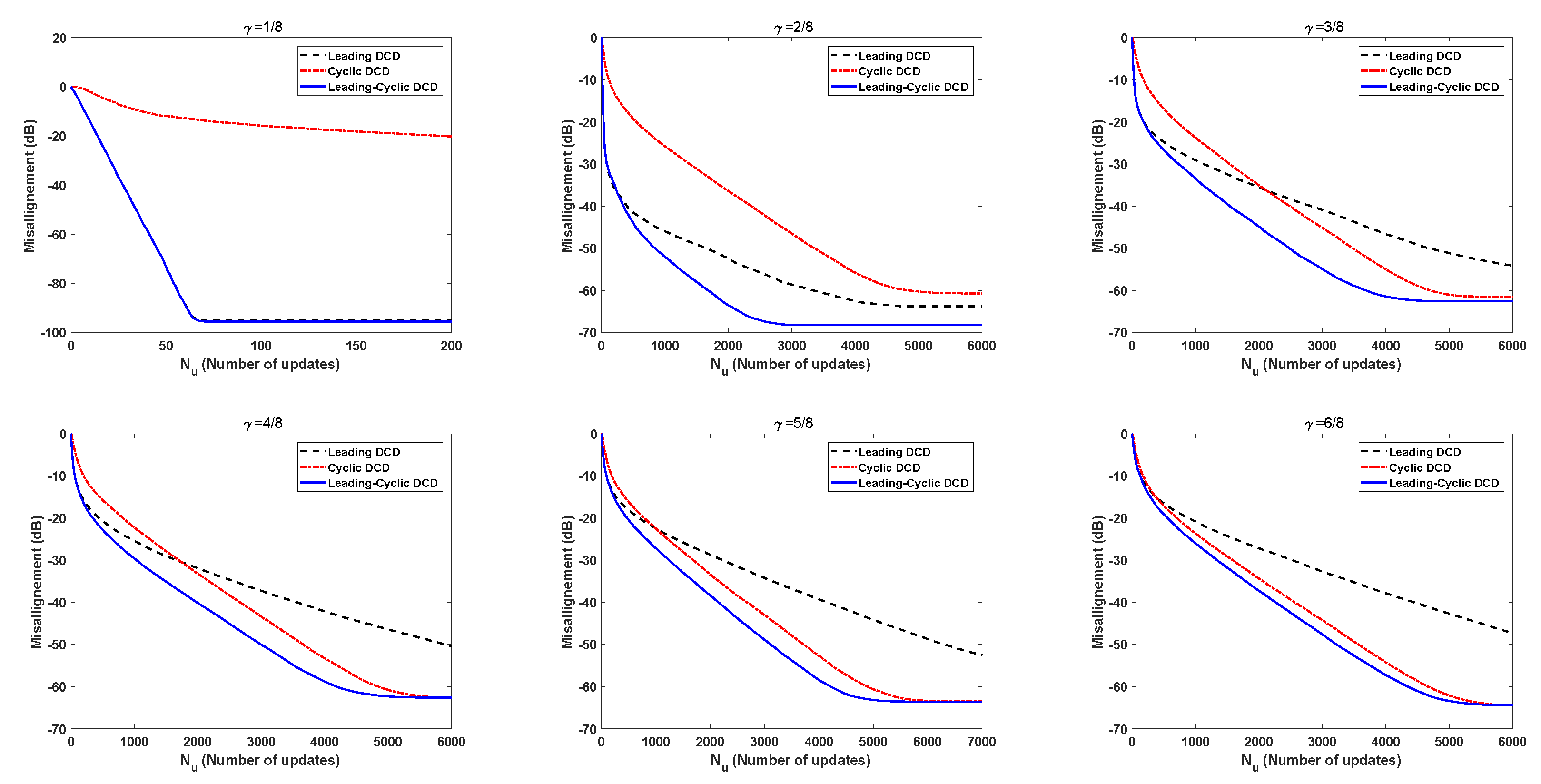
Figure 8, Figure 9, Figure 10 and Figure 11 show the misalignments of the DCD algorithms with conditional numbers of the system matrix in the interval [300, 400]. We can see that when increases, the convergence speed of the DCD algorithms decreases.
According to the numerical results above, we can see that the leading-cyclic DCD algorithm is an effective approach for solving a sparse system with a large number of updates. For example, in code division multiple access (CDMA)with a spreading factor Q, there are approximately half of the users are active in the U user system. The columns of are represented as spreading sequences. The matrix is represented as a correlation matrix of the spreading sequence.
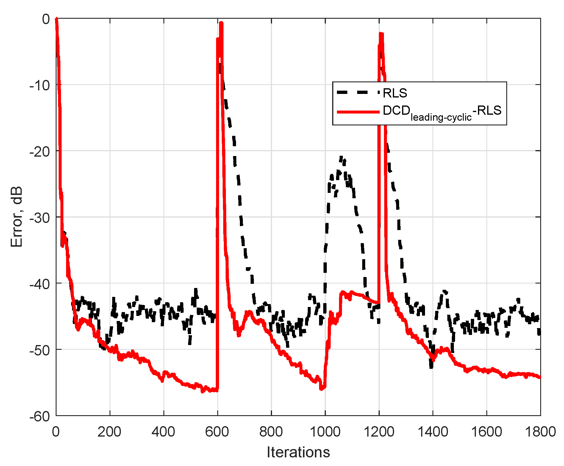
Figure 12 shows the misalignments of the RLS algorithm and DCD-RLS (forgetting factor , the length of the filter , and ). When system noise energy increases by 10 times between 1000 iterations and 1100 iterations, the DCD-RLS maintains a low error rate. The proposed algorithm-based RLS provides a lower error level and better tracking performance than the RLS algorithm.
4. Discussion
When increases, the convergence speed of the proposed algorithm (e.g., at the misalignment dB) decreases. The optimal required for solving a system of equations varies depending on the system size, the solution sparseness and the condition number of the system matrix. In this work, we choose the value that allows the proposed algorithm to achieve the fastest convergence to the steady-state level as the optimal . The results show that the optimal varies around Q and approximately remains stable with different (except for in the case of ). The ratio between Q and U in the case of is lower than those in the other cases with the same condition number range, and the leading DCD algorithm might contribute fewer iterations in the proposed algorithm to achieving the steady state when increases. Investigation of the general theory of induction for choosing the proper in the combined algorithm is left for future work.
5. Conclusions
In this paper, we have demonstrated that the leading DCD algorithm and the cyclic DCD algorithm are useful in different applications. In particular, we consider a scenario in which the sparsity of the true solution is . We propose a leading-cyclic DCD algorithm that solves normal equations with sparse solutions. The results show that the proposed leading-cyclic DCD algorithm has an optimal value in the range of and exhibits improved convergence compared to the cyclic DCD algorithm and the leading DCD algorithm. In addition, within the same range of the system matrix condition number, the larger is, the slower the convergence of the DCD algorithms.
Author Contributions
Conceptualization, Z.Q. and S.L.; methodology, Z.Q. and S.L.; software, Z.Q. and S.L.; validation, Z.Q. and S.L.; formal analysis, Z.Q. and S.L.; investigation, Z.Q. and S.L.; resources, Z.Q. and S.L.; data curation, Z.Q. and S.L.; writing—original draft preparation, Z.Q. and S.L.; writing–review and editing, Z.Q. and S.L.; visualization, Z.Q. and S.L.; supervision, Z.Q.; project administration, Z.Q.; funding acquisition, Z.Q. All authors have read and agreed to the published version of the manuscript.
Funding
This work was founded by the National Natural Science Foundation of China by Grant No. U1604160 and the China Scholarship Council.
Acknowledgments
The authors would like to thank Jie Liu for his comments and the two anonymous reviewers for their valuable suggestions.
Conflicts of Interest
The authors declare that they have no conflict of interest.
References
- Haykin, S. Adaptive Filter Theory, 4th ed.; Prentice Hall, Inc.: Upper Saddle River, NJ, USA, 2001. [Google Scholar]
- Dakulagi, V.; Bakhar, M. Advances in Smart Antenna Systems for Wireless Communication. Wirel. Pers. Commun. 2000, 110, 931–957. [Google Scholar] [CrossRef]
- Verdu, S. Multiuser Detection; Cambridge University Press: Cambridge, UK, 1998. [Google Scholar]
- Albreem, M.A.; Juntti, M.; Shahabuddin, S. Massive MIMO detection techniques: A survey. IEEE Commun. Surv. Tutor. 2019, 21, 3109–3132. [Google Scholar] [CrossRef] [Green Version]
- Messini, M.; Djendi, M. A new adaptive filtering algorithm for stereophonic acoustic echo cancellation. Appl. Acoust. 2019, 146, 345–354. [Google Scholar] [CrossRef]
- Proakis, J.; Manolakis, D. Digital Signal Processing: Principles, Algorithms, and Applications, 2nd ed.; Macmillan: New York, NY, USA, 1992. [Google Scholar]
- Wen, H.; Yang, S.; Hong, Y.; Luo, H.A. Partial Update Adaptive Algorithm for Sparse System Identification. IEEE/ACM Trans. Audio Speech Lang. Process. 2020, 28, 240–255. [Google Scholar] [CrossRef]
- Yazdanpanah, H.; Diniz, P.S.R.; Lima, M.V.S. Feature Adaptive Filtering: Exploiting Hidden Sparsity. IEEE Trans. Circuits Syst. Regul. Pap. Available online: http://www02.smt.ufrj.br/~diniz/papers/ri99.pdf (accessed on 3 June 2020). [CrossRef]
- Liu, J.; Grant, S.L. Proportionate Adaptive Filtering for Block-Sparse System Identification. IEEE/ACM Trans. Audio Speech Lang. Process. 2016, 24, 623–630. [Google Scholar] [CrossRef] [Green Version]
- Golub, G.H.; Van Loan, C.F. Matrix Computations, 3rd ed.; The Johns Hopkins University Press: Baltimore, MD, USA, 1996. [Google Scholar]
- Liu, J. DCD Algorithm: Architectures, FPGA Implementations and Applications. Ph.D. Thesis, University of York, York, UK, 2008. [Google Scholar]
- Cryer, C.W. The solution of a quadratic programming problem using systematic overrelaxation. SIAM J. Control 1971, 9, 385–392. [Google Scholar] [CrossRef]
- Watkins, D.J. Fundamentals of Matrix Computations; Wiley: Hoboken, NJ, USA, 2002. [Google Scholar]
- Quan, Z.; Tian, T. DCD-based branch and bound detector with reduced complexity for MIMO systems. IEICE Trans. Commun. 2018, E101-B, 2230–2238. [Google Scholar] [CrossRef]
- Albu, F. Efficient multichannel filtered-x affine projection algorithm for active noise control. Electron. Lett. 2006, 42, 421–423. [Google Scholar] [CrossRef]
- Albu, F.; Bouchard, M.; Zakharov, Y. Pseudo Affine Projection Algorithms for Multichannel Active Noise Control. IEEE Trans. Audio Speech Lang. Process. 2007, 15, 1044–1052. [Google Scholar] [CrossRef] [Green Version]
- Zakharov, Y. Low complexity implementation of the affine projection algorithm. IEEE Signal Process. Lett. 2008, 15, 557–560. [Google Scholar] [CrossRef]
- Zakharov, Y.; White, G.; Liu, J. Low complexity RLS algorithms using dichotomous coordinate descent iterations. IEEE Trans. Signal Process. 2008, 56, 3150–3161. [Google Scholar] [CrossRef] [Green Version]
- Zakharov, Y.V.; Tozer, T.C. Multiplication-free iterative algorithm for LS problem. Electron. Lett. 2004, 40, 567–569. [Google Scholar] [CrossRef]
- Liu, J.; Zakharov, Y.V.; Weaver, B. Architecture and FPGA design of dichotomous coordinate descent algorithms. IEEE Trans. Circuits Syst. Regul. Pap. 2009, 56, 2425–2438. [Google Scholar]
- Cotter, S.F.; Rao, B.D. Sparse channel estimation via matching pursuit with application to equalization. IEEE Trans. Commun. 2002, 50, 374–377. [Google Scholar] [CrossRef] [Green Version]
- Wu, W.C.; Chen, K.C. Identification of active users in synchronous CDMA multiuser detection. IEEE J. Sel. Areas Commun. 1998, 16, 1723–1735. [Google Scholar]
Figure 1.
Misalignments of the DCD algorithms in the system with small condition numbers in the range of [2, 5]; , , .
Figure 1.
Misalignments of the DCD algorithms in the system with small condition numbers in the range of [2, 5]; , , .

Figure 2.
Misalignments of the DCD algorithms in the system with high condition numbers in the range of [300, 400]; , , .
Figure 2.
Misalignments of the DCD algorithms in the system with high condition numbers in the range of [300, 400]; , , .

Figure 3.
Misalignments of the DCD algorithms in the system with high condition numbers in the range of and sparse solutions; , , .
Figure 3.
Misalignments of the DCD algorithms in the system with high condition numbers in the range of and sparse solutions; , , .

Figure 4.
Misalignments of the DCD algorithms in the system with the high condition numbers in the range of and sparse solutions; , , .
Figure 4.
Misalignments of the DCD algorithms in the system with the high condition numbers in the range of and sparse solutions; , , .

Figure 5.
Optimal vs. sparsity.

Figure 6.
Misalignments of the DCD algorithms for different sparse solutions with the condition numbers in the range of [100, 200] and sparse solutions; , , , .
Figure 6.
Misalignments of the DCD algorithms for different sparse solutions with the condition numbers in the range of [100, 200] and sparse solutions; , , , .

Figure 7.
Misalignments of the DCD algorithms for different sparse solutions with the condition numbers in the range of [500, 600]; , , , .
Figure 7.
Misalignments of the DCD algorithms for different sparse solutions with the condition numbers in the range of [500, 600]; , , , .

Figure 8.
Misalignments of the DCD algorithms for different sparse solutions with the condition numbers in the range of ; , , , .
Figure 8.
Misalignments of the DCD algorithms for different sparse solutions with the condition numbers in the range of ; , , , .

Figure 9.
Misalignments of the DCD algorithms for different sparse solutions with the condition numbers in the range of ; , , , .
Figure 9.
Misalignments of the DCD algorithms for different sparse solutions with the condition numbers in the range of ; , , , .

Figure 10.
Misalignments of the DCD algorithms for different sparse solutions with the condition numbers in the range of ; , , , .
Figure 10.
Misalignments of the DCD algorithms for different sparse solutions with the condition numbers in the range of ; , , , .

Figure 11.
Misalignments of the DCD algorithms for different sparse solutions with the condition numbers in the range of ; , , , .
Figure 11.
Misalignments of the DCD algorithms for different sparse solutions with the condition numbers in the range of ; , , , .

Figure 12.
Misalignments of the DCD-RLS and the RLS algorithm when there is an abrupt change in the unknown system; , , .
Figure 12.
Misalignments of the DCD-RLS and the RLS algorithm when there is an abrupt change in the unknown system; , , .


Table 1.
Cyclic DCD algorithm.
| Step | Input , R, , , ; Output: x, | Addition |
|---|---|---|
| Initialization: , , , | ||
| for | ||
| 1 | ||
| 2 | g = 0 | |
| for | ||
| 3 | if | |
| 4 | 1 | |
| 5 | U | |
| 6 | , g = 1 | |
| 7 | if , execution stops | |
| 8 | if g = 1, repeat step 2 | |
| end for | ||
| complexity | adds | |
Table 2.
Leading DCD algorithm.
| Step | Input , R, , , ; output: x, | Addition |
|---|---|---|
| Initialization: , , , | ||
| for | ||
| 1 | , goto step 4 | |
| 2 | , | |
| 3 | if , execution stops | |
| 4 | if , goto step 2 | 1 |
| 5 | 1 | |
| 6 | U | |
| end for | ||
| complexity | adds | |
Table 3.
Leading-cyclic DCD algorithm.
| Step | Input , R, , , , ; Output: x, | |
|---|---|---|
| Initialization: , , , | ||
| for | ||
| 1 | goto step 4 | |
| 2 | , | |
| 3 | if , execution stops | |
| 4 | if , goto step 2 | 1 |
| 5 | 1 | |
| 6 | ||
| 7 | end for | |
| 8 | for | |
| 9 | ||
| 10 | g = 0 | |
| 11 | for | |
| 12 | if | 1 |
| 13 | 1 | |
| 14 | U | |
| 15 | , g = 1 | |
| 16 | if , execution stops | |
| 17 | if g = 1, repeat step 10 | |
| end for | ||
| complexity | ||
| adds | ||
© 2020 by the authors. Licensee MDPI, Basel, Switzerland. This article is an open access article distributed under the terms and conditions of the Creative Commons Attribution (CC BY) license (http://creativecommons.org/licenses/by/4.0/).
Share and Cite
MDPI and ACS Style
Quan, Z.; Lv, S. Improved Convergence Speed of a DCD-Based Algorithm for Sparse Solutions. Algorithms 2020, 13, 136. https://0-doi-org.brum.beds.ac.uk/10.3390/a13060136
AMA Style
Quan Z, Lv S. Improved Convergence Speed of a DCD-Based Algorithm for Sparse Solutions. Algorithms. 2020; 13(6):136. https://0-doi-org.brum.beds.ac.uk/10.3390/a13060136
Chicago/Turabian StyleQuan, Zhi, and Shuhua Lv. 2020. "Improved Convergence Speed of a DCD-Based Algorithm for Sparse Solutions" Algorithms 13, no. 6: 136. https://0-doi-org.brum.beds.ac.uk/10.3390/a13060136
Note that from the first issue of 2016, this journal uses article numbers instead of page numbers. See further details here.