Fused Gromov-Wasserstein Distance for Structured Objects

1
CNRS, IRISA, Université Bretagne-Sud, F-56000 Vannes, France
2
CNRS, OCA Lagrange, Université Côte d’Azur, F-06000 Nice, France
3
CNRS, LETG, Université Rennes, F-35000 Rennes, France
*
Author to whom correspondence should be addressed.
Algorithms 2020, 13(9), 212; https://0-doi-org.brum.beds.ac.uk/10.3390/a13090212
Submission received: 8 July 2020
/
Revised: 20 August 2020
/
Accepted: 26 August 2020
/
Published: 31 August 2020
(This article belongs to the Special Issue Efficient Graph Algorithms in Machine Learning)
Abstract
:Optimal transport theory has recently found many applications in machine learning thanks to its capacity to meaningfully compare various machine learning objects that are viewed as distributions. The Kantorovitch formulation, leading to the Wasserstein distance, focuses on the features of the elements of the objects, but treats them independently, whereas the Gromov–Wasserstein distance focuses on the relations between the elements, depicting the structure of the object, yet discarding its features. In this paper, we study the Fused Gromov-Wasserstein distance that extends the Wasserstein and Gromov–Wasserstein distances in order to encode simultaneously both the feature and structure information. We provide the mathematical framework for this distance in the continuous setting, prove its metric and interpolation properties, and provide a concentration result for the convergence of finite samples. We also illustrate and interpret its use in various applications, where structured objects are involved.
1. Introduction
We focus on the comparison of structured objects, i.e., objects defined by both a feature and a structure information. Abstractly, the feature information cover all the attributes of an object; for example, it can model the value of a signal when objects are time series, or the node labels over a graph. In shape analysis, the spatial positions of the nodes can be regarded as features, or, when objects are images, local color histograms can describe the image’s feature information. As for the structure information, it encodes the specific relationships that exist among the components of the object. In a graph context, nodes and edges are representative of this notion, so that each label of the graph may be linked to some others through the edges between the nodes. In a time series context, the values of the signal are related to each other through a temporal structure. This representation can be related with the concept of relational reasoning (see [1]), where some entities (or elements with attributes, such as the intensity of a signal) coexist with some relations or properties between them (or some structure, as described above). Including structural knowledge about objects in a machine learning context has often been valuable in order to build more generalizable models. As shown in many contexts, such as graphical models [2,3], relational reinforcement learning [4], or Bayesian nonparametrics [5], considering objects as a complex composition of entities together with their interactions is crucial in order to learn from small amounts of data.
Unlike recent deep learning end-to-end approaches [6,7] that attempt to avoid integration of prior knowledge or assumptions about the structure wherever possible, ad hoc methods, depending on the kind of structured objects involved, aim to build meaningful tools that include structure information in the machine learning process. In graph classification, the structure can be taken into account through dedicated graph kernels, in which the structure drives the combination of the feature information [8,9,10]. In a time series context, Dynamic Time Warping and related approaches are based on the similarity between the features while allowing limited temporal (i.e., structural) distortion in the time instants that are matched [11,12]. Closely related, an entire field has focused on predicting the structure as an output and it has been deployed on tasks, such as segmenting an image into meaningful components or predicting a natural language sentence [10,13,14].
All of these approaches rely on meaningful representations of the structured objects that are involved. In this context, distributions or probability measures can provide an interesting representation for machine learning data. This allows their comparison within the Optimal Transport (OT) framework that provides a meaningful way of comparing distributions by capturing the underlying geometric properties of the space through a cost function. When the distributions dwell in a common metric space , the Wasserstein distance defines a metric between these distributions under mild assumptions [15]. In contrast, the Gromov–Wasserstein distance [16,17] aims at comparing distributions that support live in different metric spaces through the intrinsic pair-to-pair distances in each space. Unifying both distances, the Fused Gromov–Wasserstein distance was proposed in a previous work in [18] and used in the discrete setting to encode, in a single OT formulation, both feature and structure information of structured objects. This approach considers structured objects as joint distributions over a common feature space associated with a structure space specific to each object. An OT formulation is derived by considering a tradeoff between the feature and the structure costs, respectively, defined with respect to the Wasserstein and the Gromov–Wasserstein standpoints.
This paper presents the theoretical foundations of this distance and states the mathematical properties of the metric in the general setting. We first introduce a representation of structured objects using distributions. We show that classical Wasserstein and Gromov–Wasserstein distance can be used in order to compare either the feature information or the structure information of the structured object but that they both fail at comparing the entire object. We then present the Fused Gromov–Wasserstein distance in its general formulation and derive some of its mathematical properties. Particularly, we show that it is a metric in a given case, we give a concentration result, and we study its interpolation and geodesic properties. We then provide a conditional-gradient algorithm to solve the quadratic problem resulting from in the discrete case and we conclude by illustrating and interpreting the distance in several applicative contexts.
Notations. Let be the set of all probability measures on a space and the set of all Borel sets of a -algebra A. We note # the push-forward operator, such, that for a measurable function T, , .
We note supp the support of is the minimal closed subset such that . Informally, this is the set where the measure “is not zero”.
For two probability measures and we note the set of all couplings or matching measures of and , i.e., the set .
For two metric spaces and , we define the distance on such that, for .
We note the simplex of N bins as . For two histograms and we note with some abuses the set of all couplings of a and b, i.e., the set . Finally, for , denotes the dirac measure in x.
Assumption. In this paper, we assume that all metric spaces are non-trivial Polish metric spaces (i.e., separable and completely metrizable topological spaces) and that all measures are Borel.
2. Structured Objects as Distributions and Fused Gromov–Wasserstein Distance
The notion of structured objects used in this paper is inspired from the discrete point of view where one aims at comparing labeled graphs. More formally, we consider undirected labeled graphs as tuples of the form , where are the set of vertices and edges of the graph. is a labelling function that associates each vertex with a feature in some feature metric space . Similarly, maps a vertex from the graph to its structure representation in some structure space specific to each graph. is a symmetric application which aims at measuring the similarity between the nodes in the graph. In the graph context, can either encode the neighborhood information of the nodes, the edge information of the graph or more generally it can model a distance between the nodes such as the shortest path distance or the harmonic distance [19]. When is a metric, such as the shortest-path distance, we naturally endow the structure with the metric space .
In this paper, we propose enriching the previous definition of a structured object with a probability measure which serves the purpose of signaling the relative importance of the object’s elements. For example, we can add a probability (also denoted as weight) to each node in the graph. This way, we define a fully supported probability measure , which includes all the structured object information (see Figure 1 for a graphical depiction).
This graph representation for objects with a finite number of points/vertices can be generalized to the continuous case and leads to a more general definition of structured objects:
Definition 1.
(Structured objects). A structured object over a metric space is a triplet , where is a metric space and μ is a probability measure over . is denoted as the feature space, such that is the distance in the feature space and the structure space, such that is the distance in the structure space. We will note and the structure and feature marginals of μ.
Definition 2.
(Space of structured objects). We note the set of all metric spaces. The space of all structured objects over will be written as and is defined by all the triplets where and . To avoid finiteness issues in the rest of the paper we define for the space such that if we have:
(the finiteness of this integral does not depend on the choice of )
For the sake of simplicity, and when it is clear from the context, we will sometimes denote only by the whole structured object. The marginals encode very partial information since they focus only on independent feature distributions or only on the structure. This definition encompasses the discrete setting discussed in above. More precisely, let us consider a labeled graph of n nodes with features with and the structure representation of the nodes. Let be an histogram, then the probability measure defines structured object in the sense of Definition 1, since it lies in . In this case, an example of , , and is provided in Figure 1.
Note that the set of structured objects is quite general and also allows considering discrete probability measures of the form with possibly different than n. We propose focusing on a particular type of structured objects, namely the generalized labeled graphs, as described in the following definition:
Definition 3.
(Generalized labeled graph). We call generalized labeled graph a structured object such that μ can be expressed as where is surjective and pushes forward to , i.e., .
This definition implies that there exists a function , which associates a feature to a structure point and, as such, one structure point can not have two different features. The labeled graph described by is a particular instance of a generalized labeled graph in which is defined by .
2.1. Comparing Structured Objects
We now aim to define a notion of equivalence between two structured objects and . We note in the following the marginals of . Intuitively, two structured objects are the same if they share the same feature information, if their structure information are lookalike, and if the probability measures are corresponding in some sense. In this section, we present mathematical tools for individual comparison of the elements of structured objects. First, our formalism implies comparing metric spaces, which can be done via the notion of isometry.
Definition 4.
(Isometry). Let and be two metric spaces. An isometry is a surjective map that preserves the distances:
An isometry is bijective, since for we have and hence (in the same way is also a isometry). When it exists, X and Y share the same “size” and any statement about X, which can be expressed through its distance is transported to Y by the isometry f.
Example 1.
Let us consider the two following graphs whose discrete metric spaces are obtained as shortest path between the vertices (see corresponding graphs in Figure 2).
These spaces are isometric since the map f, such that , , , verifies Equation (3).
The previous definition can be used in order to compare the structure information of two structured objects. Regarding the feature information, because they all lie in the same ambient space , a natural way for comparing them is by the standard set equality . Finally, in order to compare measures on different spaces, the notion of preserving map can be used.
Definition 5.
(Measure preserving map). Let and be two measurable spaces. A function (usually called a map) is said to be measure preserving if it transports the measure on such that
If there exists such a measure preserving map, the properties about measures of are transported via f to .
Combining these two ideas together leads to the notion of measurable metric spaces (often called mm-spaces [17]), i.e., a metric space enriched with a probability measure and described by a triplet . An interesting notion for comparing mm-spaces is the notion of isomorphism.
Definition 6.
(Isomorphism). Two mm-spaces are isomorphic if there exists a surjective measure preserving isometry between the support of the measures .
Example 2.
Let us consider two mm-spaces and , as depicted in Figure 3. These spaces are isometric, but not isomorphic, as there exists no measure preserving map between them.
All of this considered, we can now define a notion of equivalence between structured objects.
Definition 7.
(Strong isomorphism of structured objects).
Two structured objects are said to be strongly isomorphic if there exists an isomorphism I between the structures such that is bijective between and and measure preserving. More precisely, f satisfies the following properties:
- P.1
- .
- P.2
- The function f statisfies:
- P.3
- The function is surjective, satisfies and:
It is easy to check that the strong isomorphism defines an equivalence relation over .
Remark 1.
The function f described in this definition can be seen as a feature, structure, and measure preserving function. Indeed, fromP.1f is measure preserving. Moreover, and are isomorphic through I. Finally usingP.1andP.2we have that , so that the feature information is also preserved.
Example 3.
To illustrate this definition, we consider a simple example of two discrete structured objects:
with for i, and for , (see Figure 4). The two structured objects have isometric structures and same features individually, but they are not strongly isomorphic. One possible map , such that leads to an isometry is , , , . Yet, this map does not satisfy for any x, since and . The other possible functions, such that leads to an isometry are simply permutations of this example, yet it is easy to check that none of them verifiesP.2(for example, with ).
2.2. Background on OT Distances
The Optimal Transport (OT) framework defines distances between probability measures that describe either the feature or the structure information of structured objects.
Wasserstein distance. The classical OT theory aims at comparing probability measures . In this context the quantity:
is usually called the p-Wasserstein distance (also known, for , as Earth Mover’s distance [20] in the computer vision community) between distributions and . It defines a distance on probability measures, especially iff . This distance also has a nice geometrical interpretation as it represents an optimal cost (w.r.t. d) to move the measure onto with the amount of probability mass shifted from a to b (see Figure 5). To this extent, the Wasserstein distance quantifies how “far” is from by measuring how “difficult” it is to move all the mass from onto . Optimal transport can deal with smooth and discrete measures and it has proved to be very useful for comparing distributions in a shared space, but with different (and even non-overlapping) supports.
Gromov–Wasserstein distance. In order to compare measures whose support are not necessarily in the same ambient space [16,17] define a new OT distance. By relaxing the classical Hausdorff distance [15,17], authors build a distance over the space of all mm-spaces. For two compact mm-spaces and , the Gromov–Wasserstein distance is defined as:
where:
The Gromov–Wasserstein distance depends on the choice of the metrics and and with some abuse of notation we denote the entire mm-space by its probability measure. When it is not clear from the context, we will specify using . The resulting coupling tends to associate pairs of points with similar distances within each pair (see Figure 6). The Gromov–Wasserstein distance allows for the comparison of measures over different ground spaces and defines a metric over the space of all mm-spaces quotiented by the isomoprhisms (see Definitions 4 and 5). More precisely, it vanishes if the two mm-spaces are isomorphic. This distance has been used in the context of relational data e.g., in shape comparison [17,22], deep metric alignment [23], generative modelling [24] or to align single-cell multi-omics datasets [25].
2.3. Fused Gromov–Wasserstein Distance
Building on both Gromov–Wasserstein and Wasserstein distances, we define the Fused Gromov–Wasserstein () distance on the space of structured objects:
Definition 8.
(Fused Gromov-Wasserstein distance). Let and . We consider and . The Fused-Gromov–Wasserstein distance is defined as:
where
Figure 7 illustrates this definition. When it is clear from the context we will simply note instead for for brevity. acts as a trade-off parameter between the cost of the structures represented by and the feature cost . In this way, the convex combination of both terms leads to the use of both information in one formalism resulting on a single map that “moves” the mass from one joint probability measure to the other.
Many desirable properties arise from this definition. Among them, one can define a topology over the space of structured objects using the distance to compare structured objects, in the same philosophy as for Wasserstein and Gromov–Wasserstein distances. The definition also implies that acts as a generalization of both Wasserstein and Gromov-Wasserstein distances, with achieving an interpolation between these two distances. More remarkably, distance also realizes geodesic properties over the space of structured objects, allowing the definition of gradient flows. All of these properties are detailed in the next section. Before reviewing them, we first compare with and W (by assuming for now that exists, which will be shown later in Theorem 1).
Proposition 1.
(Comparaison between , and W). We have the following results for two structured objects μ and ν:
- The following inequalities hold:
- Let us suppose that the structure spaces , are part of a single ground space (i.e., and ). We consider the Wasserstein distance between μ and ν for the distance on : . Then:
Proof of this proposition can be found in Section 7.1. In particular, following this proposition, when the distance vanishes then both and W distances vanish so that the structure and the feature of the structure object are individually “the same” (with respect to their corresponding equivalence relation). However, the converse is not necessarily true, as shown in the following example.
Example 4.
(Toy trees). We construct two trees as illustrated in Figure 8 where the 1D node features are shown with colors. The shortest path between the nodes is used to capture the structures of the two structured objects and the Euclidean distance is used for the features. We consider uniform weights on all nodes. Figure 8 illustrates the differences between , , and W distances. The left part is the Wasserstein coupling between the features: red nodes are transported on red ones and the blue nodes on the blue ones but tree structures are completely discarded. In this case, the Wasserstein distance vanishes. In the right part, we compute the Gromov–Wasserstein distance between the structures: all couples of points are transported to another couple of points, which enforces the matching of tree structures without taking into account the features. Because structures are isometric, the Gromov–Wasserstein distance is null. Finally, we compute the using intermediate α (center), the bottom and first level structure is preserved as well as the feature matching (red on red and blue on blue) and discriminates the two structured objects.
3. Mathematical Properties of
In this section, we establish some mathematical properties of the distance. The first result relates to the existence of the distance and the topology of the space of structured objects. We then prove that the distance is indeed a distance regarding the equivalence relation between structured objects, as defined in Defintion 7, allowing us to derive a topology on .
3.1. Topology of the Structured Object Space
The distance has the following properties:
Theorem 1.
(Metric properties). Let , and . The functional always achieves an infimum in s.t. . Moreover:
- •
- is symmetric and, for , satisfies the triangle inequality. For , the triangular inequality is relaxed by a factor .
- •
- For , if an only if there exists a bijective function such that:
- •
- If are generalized labeled graphs then if and only if and are strongly isomorphic.
Proof of this theorem can be found in Section 7.2. The identity of indiscernibles is the most delicate part to prove and it is based on using the Gromov–Wasserstein distance between the spaces and . The previous theorem states that is a distance over the space of generalized labeled graphs endowed with the strong isomorphism as equivalence relation defined in Definition 7. More generally, for any structured objects the equivalence relation is given by (12)–(14). Informally, invariants of the are structured objects that have both the same structure and the same features in the same place. Despite the fact that leads to a proper metric, we will further see in Section 4.1 that the case can be computed more efficiently using a separability trick from [26].
Theorem 1 allows a wide set of applications for , such as k-nearest-neighbors, distance-substitution kernels, pseudo-Euclidean embeddings, or representative-set methods [27,28,29]. Arguably, such a distance allows for a better interpretation than to end-to-end learning machines, such as neural networks, because the matrix exhibits the relationships between the elements of the objects in a pairwise comparison.
3.2. Can We Adapt W and GW for Structured Objects?
Despite the appealing properties of both Wasserstein and Gromov–Wasserstein distances, they fail at comparing structured objects by focusing only on the feature and structure marginals, respectively. However, with some hypotheses, one could adapt these distances for structured objects.
Adapting Wasserstein. If the structure spaces and are part of a same ground space , i.e., ( and ), one can build a distance between couples and and apply the Wasserstein distance, so as to compare the two structured objects. In this case, when the Wasserstein distance vanishes it implies that the structured objects are equal in the sense . This approach is very related with the one discussed in [30], where the authors define the Transportation distance for signal analysis purposes. Their approach can be viewed as a transport between two joint measures , for function representative of the signal values and the Lebesgue measure. The distance for the transport is defined as for and the norm. In this case, and can be interpreted as encoding the feature information of the signal, while encode its structure information. This approach is very interesting, but cannot be used on structured objects, such as graphs that will not share a common structure embedding space.
Adapting Gromov-Wasserstein. The Gromov–Wasserstein distance can also be adapted to structured objects by considering the distances and within each space and , respectively, and . When the resulting distance vanishes, structured objects are isomorphic with respect to and . However, the strong isomorphism is stronger than this notion, since the isomorphism allows for “permuting the labels”, but not the strong isomorphism. More precisely, we have the following lemma:
Lemma 1.
Let be two structured objects and .
If and are strongly isomorphic then and are isomorphic. However the converse is not true in general.
Proof.
To see this, if we consider f as defined in Theorem 1, then, for , we have . In this way:
which can be rewritten as:
and so f is an isometry with respect to and . Because f is also measure preserving and surjective and are isomorphic. □
However, the converse is not necessarily true, as it is easy to cook up an example with the same structure but with permuted labels, so that objects are isomorphic but not strongly isomorphic. For example, in the tree example Figure 4, the structures are isomorphic and the distances between the features within each space are the same between each structured objects, so that and are isomorphic, yet not strongly isomorphic, as shown in the example since .
3.3. Convergence of Structured Objects
The metric property naturally endows the structured object space with a notion of convergence, as described in the next definition:
Definition 9.
Convergence of structured objects.
Let be a sequence of structured objects. It converges to in the Fused Gromov–Wasserstein sense if:
Using Proposition 1, it is straightforward to see that if the sequence converges in the sense, both the features and the structure converge respectively in the Wasserstein and Gromov–Wasserstein sense (see [17] for the definition of convergence in the Gromov–Wasserstein sense).
An interesting question arises from this definition. Let us consider a structured object and let us sample the joint distribution so as to consider with where are sampled from . Does this sequence converges to in the sense and how fast is the convergence?
This question can be answered thanks to a notion of “size” of a probability measure. For the sake of conciseness, we will not exhaustively present the theory, but the reader can refer to [31] for more details. Given a measure on , we denote as its upper Wasserstein dimension. It coincides with the intuitive notion of “dimension” when the measure is sufficiently well behaved. For example, for any absolutely continuous measure with respect to the Lebesgue measure on , we have for any . Using this definition and the results presented in [31], we answer the question of convergence of finite sample in the following theorem (proof can be found in Section 7.3):
Theorem 2.
Convergence of finite samples and a concentration inequality
Let . We have:
Moreover, suppose that . Then there exists a constant C that does not depend on n such that:
The expectation is taken over the i.i.d samples . A particular case of this inequality is when so that we can use the result above to derive a concentration result for the Gromov-Wasserstein distance. More precisely, if denotes the empirical measure of and if , we have:
This result is a simple application of the convergence of finite sample properties of the Wasserstein distance, since in this case and are part of the same ground space so that (18) derive naturally from (11) and the properties of Wasserstein. In contrast to the Wasserstein distance case, this inequality is not necessarily sharp and future work will be dedicated to the study of its tightness.
3.4. Interpolation Properties between Wasserstein and Gromov-Wasserstein Distances
distance is a generalization of both Wasserstein and Gromov–Wasserstein distances in the sense that it achieves an interpolation between them. More precisely, we have the following theorem:
Theorem 3.
Interpolation properties.
As α tends to zero, one recovers the Wasserstein distance between the features information and as α goes to one, one recovers the Gromov–Wasserstein distance between the structure information:
Proof of this theorem can be found in Section 7.4.
This result shows that can revert to one of the other distances. In machine learning, this allows for a validation of the parameter to better fit the data properties (i.e., by tuning the relative importance of the feature vs. structure information). One can also see the choice of as a representation learning problem and its value can be found by optimizing a given criterion.
3.5. Geodesic Properties
One desirable property in OT is the underlying geodesics defined by the mass transfer between two probability distributions. These properties are useful in order to define the dynamic formulation of OT problems. This dynamic point of view is inspired by fluid dynamics and found its origin in the Wasserstein context with [32]. Various applications in machine learning can be derived from this formulation: interpolation along geodesic paths were used in computer graphics for color or illumination interpolations [33]. More recently, Ref. [34] used Wasserstein gradient flows in an optimization context, deriving global minima results for non-convex particles gradient descent. In [35], the authors used Wasserstein gradient flows in the context of reinforcement learning for policy optimization.
The main idea of this dynamic formulation is to describe the optimal transport problem between two measures as a curve in the space of measures minimizing its total length. We first describe some generality about geodesic spaces and recall classical results for dynamic formulation in both Wasserstein and Gromov–Wasserstein contexts. In a second part, we derive new geodesic properties in the context.
Geodesic spaces. Let be a metric space and two points in X. We say that a curve joining the endpointsx and y (i.e., with and ) is a constant speed geodesic if it satisfies for . Moreover, if is a length space (i.e., if the distance between two points of X is equal to the infimum of the lengths of the curves connecting these two points) then the converse is also true and a constant speed geodesic satisfies . It is easy to compute distances along such curves, as they are directly embedded into .
In the Wasserstein context, if the ground space is a complete separable, locally compact length space, and if the endpoints of the geodesic are given, then there exists a geodesic curve. Moreover, if the transport between the endpoints is unique, then there is a unique displacement interpolation between the endpoints (see Corollary 7.22 and 7.23 in [15]). For example, if the ground space is and the distance between the points is measured via the norm, then geodesics exist and are uniquely determined (this can be generalized to strictly convex costs). In the Gromov–Wasserstein context, there always exists constant speed geodesics as long as the endpoints are given. These geodesics are unique modulo the isomorphism equivalence relation (see [16]).
The case. In this paragraph, we suppose that . We are interested in finding a geodesic curve in the space of structured objects i.e., a constant speed curve of structured objects joining two structured objects. As for Wasserstein and Gromov–Wasserstein, the structured object space endowed with the Fused Gromov–Wasserstein distance maintains some geodesic properties. The following result proves the existence of such a geodesic and characterizes it:
Theorem 4.
Constant speed geodesic.
Let and and in . Let be an optimal coupling for the Fused Gromov–Wasserstein distance between , and . We equip with the norm for .
We define such that:
Then:
is a constant speed geodesic connecting and in the metric space .
Proof of the previous theorem can be found in Section 7.5. In a sense, this result combines the geodesics in the Wasserstein space and in the space of all mm-spaces, since it suffices to interpolate the distances in the structure space and the features to construct a geodesic. The main interest is that it defines the minimum path between two structured objects. For example, when considering two discrete structured objects represented by the measures and , the interpolation path is given for by the measure where is an optimal coupling for the distance. However this geodesic is difficult to handle in practice, since it requires the computation of the cartesian product . To overcome this obstacle, an extension using theFréchet mean is defined in Section 4.2. The proper definition and properties of velocity fields associated to this geodesic is postponed to further works.
4. in the Discrete Case
In practice, structured objects are often discrete and can be defined using the labeled graph formalism described previously. In this section, we discuss how to compute efficiently. We also provide an algorithm for the computation of Fréchet means.
4.1. FGW in the Discrete Case
We consider two structured objects and , as described previously. We note the matrix and the matrices , (see Figure 9). The Fused Gromov–Wasserstein distance is defined as
where:
Solving the related Quadratic Optimization problem. Equation (24) is clearly a quadratic problem w.r.t. . Note that, despite the apparent complexity of computing the tensor product, one can simplify the sum to complexity [26] when considering . In this case, the computation problem can be re-written as finding , such that:
where and . denote the Kronecker product of two matrices, vec the column-stacking operator. With such form, the resulting optimal map can be seen as a quadratic regularized map from initial Wasserstein [36,37]. However, unlike these approaches, we have a quadratic but probably non-convex term. The gradient G that arises from Equation (24) can be expressed with the following partial derivative w.r.t.:
Solving a large scale QP with a classical solver can be computationally expensive. In [36], the authors propose a solver for a graph regularized optimal transport problem whose resulting optimization problem is also a QP. We can then directly use their conditional gradient defined in Algorithm 1 to solve our optimization problem. It only needs at each iteration to compute the gradient in Equation (26) and solve a classical OT problem for instance with a network flow algorithm. The line-search part is a constrained minimization of a second degree polynomial function that is adapted to the non convex loss in Algorithm 2. While the problem is non convex, conditional gradient is known to converge to a local stationary point [38]. When are squared Euclidean distance matrices the problem reduces to a concave graph matching so that the line-search of the conditional gradient Algorithm 1 always leads to 1 [39,40].
| Algorithm 1. Conditional Gradient (CG) for . |
| Algorithm 2. Line-search for CG (). |
|
4.2. Structured Optimal Transport Barycenter
An interesting use of the distance is to define a barycenter of a set of structured data as a Fréchet mean. In that context, one seeks the structured object that minimizes the sum of the (weighted) distances with a given set of objects. OT barycenters have many desirable properties and applications [26,41], yet no formulation can leverage both structural and feature information in the barycenter computation. Here, we propose to use the distance to compute the barycenter of a set of K structured objects associated with structures , features and base histograms .
We suppose that the feature space is and . For simplicity, we assume that the base histograms and the histogram h associated to the barycenter are known and fixed. Note that it could be also included in the optimization process, as suggested in [26].
In this context, for a fixed and , such that , we aim to find:
Note that this problem is convex w.r.t. C and A, but not w.r.t.. Intuitively, looking for a barycenter means finding feature values supported on a fixed size support, and the structure that relates them. Interestingly enough, there are several variants of this problem, where features or structure can be fixed for the barycenter. Solving the related simpler optimization problems extend straightforwardly.
Solving the barycenter problem with Block Coordinate Descent (BCD). We propose minimizing Equation (27) using a BCD algorithm, i.e., iteratively minimizing with respect to the couplings , the structure metric C and the feature vector A.The minimization of this problem w.r.t. is equivalent to computing K independent Fused Gromov–Wasserstein distances using the algorithm presented above. We suppose that the feature space is and we consider . Minimization w.r.t. C in this case has a closed form (see Prop. 4 in [26]):
where h is the histogram of the barycenter and the division is computed pointwise. Minimization w.r.t. A can be computed with (Equation (8) in [42]):
5. Examples and Applications
In this section we derive some applications of in graph contexts such as classification, clustering and coarsening of graphs.
5.1. Illustrations of FGW
In this section, we present several applications of as a distance between structured objects and provide an interpretation of the OT matrix.
Example with one-dimensional (1D) features and structure spaces.Figure 10 illustrates the differences between Wasserstein, Gromov–Wasserstein, and Fused Gromov–Wasserstein couplings . In this example, both the feature and structure space are one-dimensional (Figure 10 left). The feature space (vertical axis) denotes two clusters among the elements of both objects illustrated in the OT matrix , the structure space (horizontal axis) denotes a noisy temporal sequence along the indexes illustrated in the matrices and (Figure 10 center). Wasserstein respects the clustering, but forgets the temporal structure, Gromov–Wasserstein respects the structure, but do not take the clustering into account. Only FGW retrieves a transport matrix respecting both feature and structure.
Example on two simple images. We extract a image from the MNIST dataset and generate a second one through translation or mirroring of the digit in the original image. We use pixel gray levels of the pixels as the features, and the structure is defined as the city-block distance on the pixel coordinate grid. We use equal weights for all of the pixels in the image. Figure 11 shows the different couplings obtained when only considering either the features, the structure only or both information. aligns the pixels of the digits, recovering the correct order of the pixels, while both Wassertein and Gromov–Wasserstein distances fail at providing a meaningful transportation map. Note that in the Wasserstein and Gromov-Wasserstein case, the distances are equal to 0, whereas manages to spot that the two images are different. Additionally, note that, in the sense, the original digit and its mirrored version are also equivalent as there exists an isometry between their structure spaces, making invariant to rotations or flips in the structure space in this case.
Example on time series data. One of the main assets of is that it can be used on a wide class of objects and time series are one more example of this. We consider here 25 monodimensional time series composed of two humps in with random uniform height between 0 and 1. The signals are distributed according to two classes translated from each other with a fixed gap. The distance is computed by considering d as the euclidean distance between the features of the signals (here the value of the signal in each point) and and as the euclidean distance between timestamps.
A two-dimensional (2D) embedding is computed from a distance matrix between a number of examples in this dataset with multidimensional scaling (MDS) [43] in Figure 12 (top). One can clearly see that the representation with a reasonable value in the center is the most discriminant one. This can be better understood by looking as the OT matrices between the classes. Figure 12 (bottom) illustrates the behavior of on one pair of examples when going from Wasserstein to Gromov–Wasserstein. The black line depicts the matching provided by the transport matrix and one can clearly see that while Wasserstein on the left assigns samples completely independently to their temporal position, the Gromov-Wasserstein on the right tends to align perfectly the samples (note that it could have reversed exactly the alignment with the same loss), but discards the values in the signal. Only the true in the center finds a transport matrix that both respects the time sequences and aligns similar values in the signals.
5.2. Graph-Structured Data Classification
In this section, we adress the question of training a classifier for graph data and evaluate the FGW distance used in a kernel with SVM.
Learning problem and datasets. We consider 12 widely used benchmark datasets divided into 3 groups. BZR, COX2 [44], PROTEINS, ENZYMES [45], CUNEIFORM [46] and SYNTHETIC [47] are vector attributed graphs. MUTAG [48], PTC-MR [49], and NCI1 [50] contain graphs with discrete attributes derived from small molecules. IMDB-B, IMDB-M [51] contain unlabeled graphs derived from social networks. All of the datasets are available in [52].
Experimental setup. Regarding the feature distance matrix between node features, when dealing with real valued vector attributed graphs, we consider the distance between the labels of the vertices. In the case of graphs with discrete attributes, we consider two settings: in the first one, we keep the original labels (denoted as raw); we also consider a Weisfeiler-Lehman labeling (denoted as wl) by concatenating the labels of the neighbors. A vector of size h is created by repeating this procedure h times [49,53]. In both cases, we compute the feature distance matrix by using where if else and denotes the concatenated label at iteration k (for original labels are used). Regarding the structure distances C, they are computed by considering a shortest path distance between the vertices.
For the classification task, we run a SVM using the indefinite kernel matrix , which is seen as a noisy observation of the true positive semidefinite kernel [54]. We compare classification accuracies with the following state-of-the-art graph kernel methods: (SPK) denotes the shortest path kernel [45], (RWK) the random walk kernel [55], (WLK) the Weisfeler Lehman kernel [53], and (GK) the graphlet count kernel [56]. For real valued vector attributes, we consider the HOPPER kernel (HOPPERK) [47] and the propagation kernel (PROPAK) [57]. We build upon the GraKel library [58] to construct the kernels and C-SVM to perform the classification. We also compare with the PATCHY-SAN framework for CNN on graphs (PSCN) [9] building on our own implementation of the method.
To provide a comparison between the methods, most of the papers about graph classification usually perform a nested cross validation (using nine-fold for training, one for testing, and reporting the average accuracy of this experiment repeated 10 times), and report accuracies of the other methods taken from the original papers. However, these comparisons are not fair because of the high variance (on most datasets) w.r.t. the folds chosen for training and testing. This is why, in our experiments, the nested cross validation is performed on the same folds for training and testing for all methods [59]. In the result, Table 1, Table 2 and Table 3, we write in bold the best score for each dataset and we add a (*) when the best score does not yield to a significative improvement (based on a Wilcoxon signed rank test on the test scores) compared to the second best one. Note that, because of their small sizes, we repeat the experiments 50 times for MUTAG and PTC-MR datasets. For all methods using SVM, we cross validate the parameter . The range of the WL parameter h is , and we also compute this kernel with h fixed at . The decay factor for RWK , for the GK kernel we set the graphlet size and cross validate the precision level and the confidence as in the original paper [56]. The parameter for PROPAK is chosen within . For PSCN, we choose the normalized betweenness centrality as labeling procedure and cross validate the batch size in and number of epochs in . Finally, for , is cross validated within and is cross validated via a logspace search in and symmetrically (15 values are drawn).
Vector attributed graphs. The average accuracies reported in Table 1 show that FGW is a clear state-of-the-art method and performs best on four out of six datasets with performances in the error bars of the best methods on the other two datasets. The results for CUNEIFORM are significantly below those from the original paper [46], which can be explained by the fact that the method in this paper uses a graph convolutional approach specially designed for this dataset and that experiment settings are different. In comparison, the other competitive methods are less consistent, as they exhibit some good performances on some datasets only.
Discrete labeled graphs. We first note in Table 2 that using WL attributes outperforms all competitive methods, including with raw features. Indeed, the WL attributes allow for more finely encoding the neighborood of the vertices by stacking their attributes, whereas FGW with raw features only consider the shortest path distance between vertices, not their sequence of labels. This result calls for using meaningful feature and/or structure matrices in the FGW definition, which can be dataset-dependant, in order to enhance the performances. We also note that with WL attributes outperforms the WL kernel method, highlighting the benefit of an optimal transport-based distance over a kernel-based similarity. Surprisingly, the results of PSCN are significantly lower than those from the original paper. We believe that it comes from the difference between the fold assignment for training and testing, which suggests that PSCN is difficult to tune.
Non-attributed graphs. The particular case of the GW distance for graph classification is also illustrated on social datasets, which contain no labels on the vertices. Note that no artificial features were added to these datasets. Accuracies reported in Table 3 show that it greatly outperforms the SPK and GK graph kernel methods. This is, to the best of our knowledge, the first application of the Gromov–Wasserstein distance for social graph classification and it highlights the fact that is a good metric for comparing the graph structures.
Comparison between , W and . During the validation step, the optimal value of was consistently selected inside the interval, i.e., excluding 0 and 1, suggesting that both structure and feature information are necessary.
5.3. Graph Barycenter and Compression
In this experiment, we use to compute barycenters and approximations of toy graphs. In the first example, we generate graphs following either a circle or 8 symbol with 1D features following a sine and linear variation, respectively. For each example, the number of nodes is drawn randomly between 10 and 25, Gaussian noise is added to the features and a small noise is applied to the structure (some connections are randomly added). An example graph with no noise is provided for each class in the first column of Figure 13. One can see from there that the circle class has a feature varying smoothly (sine) along the graph, but the 8 has a sharp feature change at its center (so that low pass filtering would loose some information). Some examples of the generated graphs are provided in the 2nd-to-7th columns of Figure 13. We compute the barycenter containing 10 samples while using the shortest path distance between the nodes as the structural information and the distance for the features. We recover an adjacency matrix by thresholding the similarity matrix C given by the barycenter. The threshold is tuned, so as to minimize the Frobenius norm between the original C matrix and the shortest path matrix constructed after thresholding C. Resulting barycenters are showed in Figure 13 for and nodes. First, one can see that the barycenters are denoised in both the feature space and structure space. Also note that the sharp change at the center of the 8 class is conserved in the barycenters, which is a nice result when compared to other divergences that tend to smooth-out their barycenters (, for instance). Finally, note that, by selecting the number of nodes in the barycenter, one can compress the graph or estimate a “high resolution” representation from all the samples. To the best of our knowledge, no other method can compute such graph barycenters. Finally, note that is interpretable, because the resulting OT matrix provides correspondence between the nodes from the samples and those from the barycenter.
In the second experiment, we evaluate the ability of FGW to perform graph approximation and compression on a Stochastic Block Model graph [60,61]. The question is to see whether estimating an approximated graph can recover the relation between the blocks and perform simultaneously a community clustering on the original graph (using the OT matrix). We generate two community graphs illustrated in the left column of Figure 14. We can see that the relation between the blocks is sparse and has a “linear” structure, the example in the first line has features that follow the blocks (noisy but similar in each block) whereas the example in the second line has two modes per block. The first graph approximation (top line) is done with four nodes and we can recover both the blocks in the graph and the average feature on each blocks (colors on the nodes). The second problem is more complex due to the two modes per block but one can see that when approximating the graph with eight nodes we recover both the structure between the blocks and the sub-clusters in each block, which illustrates the strength of that encodes both features and structures.
5.4. Unsupervised Learning: Graphs Clustering
In the last experiment, we evaluate the ability of to perform a clustering of multiple graphs and to retrieve meaningful barycenters of such clusters. To do so, we generate a dataset of four groups of community graphs. Each graph follows a simple Stochastic Block Model [60,61] and the groups are defined w.r.t. the number of communities inside each graph and the distribution of their labels. More precisely, labels are drawn from a 1D gaussian distribution specific to each community: each feature of a node is drawn from a law , where is the index of the community and to create two modes per community. The dataset is composed of 40 graphs (10 graphs per group) and the number of nodes of each graph is drawn randomly from , as illustrated in Figure 15. We perform a k-means clustering using the barycenter defined in Equation (27) as the centroid of the groups and the distance for the cluster assignment. We set the number of nodes of each centroid to 30. We perform a thresholding on the pairwise similarity matrix C of the centroid at the end in order to obtain an adjacency matrix for visualization purposes. The threshold value is chosen, so as to minimize the distance that is induced by the Frobenius norm between the original matrix C and the shortest path matrix obtained from the adjacency matrix. The evolution of the barycenters along the iterations is reported in Figure 15. We can see that these centroids recover community structures and feature distributions that are representative of their cluster content. On this example, note that the clustering perfectly recovers the known groups in the dataset. To the best of our knowledge, there exists no other method that is able to perform a clustering of graphs of arbitrary size and to retrieve the average graph in each cluster without having to solve a pre-image problem.
6. Conclusions
This paper presents the Fused Gromov–Wasserstein () distance. Inspired by both Wasserstein and Gromov–Wasserstein distances, can compare structured objects by including the inherent relations that exist between the elements of the objects, constituting their structure information, and their feature information, part of a common ground space between each structured objects. We have stated mathematical results about this new distance, such as metric, interpolation, and geodesic properties. We have also provided a concentration result for the convergence of finite samples. In the discrete case, algorithms to compute itself and related Fréchet means are provided. The use of this new distance is illustrated on problems involving structured objects, such as time series embedding, graph classification, graph barycenter computation, and graph clustering. Several questions are raised by this work. From a practical side, the FGW method is quite expensive to compute and further works will try to lower the computational complexity of the underlying optimization problem to ensure better scalability to very large graphs. Moreover, while we mostly consider in this work structure of graphs described by the shortest path, other choices could be made, such as the distances based on the Laplacian of the graph. Finally, from a theoretical point of view, it is often valuable that the geodesic path be unique, so as to defined properly objects, such as gradient flows. One interesting result would be, for example, to see if the geodesic is unique with respect to the strong isomorphism relation.
7. Proofs of the Mathematical Properties
This section presents all of the proofs of previous theorems and results. We note the projection on the i-th marginal of . We will frequently use the following lemma:
Lemma 2.
Let . We have:
Proof.
Indeed, if
Last inequality is a consequence of HÃlder inequality. The result remains valid for . □
7.1. Proof of Proposition 1—Comparison between FGW, GW and W
Proof.
Of the Proposition.
For the two inequalities (9) and (10), let be an optimal coupling for the Fused Gromov-Wasserstein distance between and (assuming its existence for now). Clearly:
Becasue the coupling is in . So by suboptimality:
which proves Equation (9). Same reasoning is used for Equation (10).
For the last inequality (11), let be any admissible coupling. By suboptimality:
(*) is the triangle inequality of and (**) Minkowski inequality. Since this inequality is true for any admissible coupling we can apply it with the optimal coupling for the Wasserstein distance defined in the proposition and the claim follows. □
7.2. Proof of Theorem 1—Metric Properties of FGW
We prove the theorem point by point: first the existence, then the equality relation and finally the triangle inequality statement. We first recall the definition of weak convergence of probability measure in a metric space [62]:
Definition 10.
(Weak-convergence on a metric space). Let be a sequence of probability measures on where is a completely metrizable topological space (Polish space) and is the Borel σ algebra. We say that converges weakly to μ in if for all continuous and bounded functions :
We also recall the definition of semi continuity in a metric space:
Definition 11.
(Lower-semi continuity). On a metric space a function is said to be lower semi-continuous (l.s.c.) if for every sequence we have .
To state the existence of a minimizer, we will rely on the following lemma:
Lemma 3.
Let W be a Polish space. If is lower semi-continuous, then the functional with is l.s.c. for the weak convergence of measures.
Proof.
f is l.s.c. and bounded from below by 0. We can consider a sequence of continuous and bounded functions converging increasingly to f (see e.g., [63]). By the monotone convergence theorem .
Moreover every is continuous for the weak convergence. Using Theorem 2.8 [62] on the Polish space we know that if converges weakly to then the product measure converges weakly to . In this way since are continuous and bounded. In particular every is l.s.c.
Proposition 2.
Existence of an optimal coupling for the distance. For , always achieves a infimum in such that .
Proof.
Since and are Polish spaces we known that is compact (Theorem 1.7 in [63]), so by applying Weierstrass theorem we can conclude that the infimum is attained at some if is l.s.c.
We will use Lemma 3 to prove that the functionnal is l.s.c. on . If we consider which is a a metric space endowed with the distance and then f is l.s.c. by continuity of d, and . With the previous reasoning we can conclude that the infimum is attained. Finally finiteness come from:
where in (*) we used Lemma 30 and in (**) that are in . □
Proposition 3.
Equality relation. For , if an only if there exists a bijective function such that:
Moreover if are generalized labeled graphs then if and only if and are strongly isomorphic.
Proof.
For the first point, let us assume that there exists a function f verifying (33)–(35). We consider the map . We note . Then:
Conversely, suppose that . To prove the existence of a map verifying (33)–(35) we will use the Gromov-Wasserstein properties. We are looking for a vanishing Gromov-Wassersein distance between the spaces and equipped with our two measures and .
More precisely, we define for and :
and
We will prove that . To show that we will bound the Gromov cost with the metrics by the Gromov cost with the metrics and a Wasserstein cost.
Let be any admissible transportation plan. Subsequently, for :
using Jensen inequality with convexity of and subadditivity of |.|. We note the first term above and the second term above. By the triangle inequality property of d we have:
(**) such that we have shown:
Now let be an optimal coupling for between and . By hypothesis so that:
and:
Subsequently, which implies that d is zero a.e. so that for any . In this way:
Using Equation (37), we have shown
which implies that for the coupling .
Thanks to the Gromov–Wasserstein properties (see [17]) this states the existence of an isometry between and . So there exists a surjective function , which verifies P.1 and:
or equivalently:
In particular, is concentrated on or equivalently . Injecting in (39) leads to:
Which implies:
Moreover, using the equality (41), we can conclude that:
Moreover, suppose that and are generalized labeled graphs. In this case there exists surjective such that . Afterwards, (44) implies that:
We define such that . Then we have by (45) for . Overall we have for all . Also since we have .
Moreover, I is a surjective function. Indeed let . Let such that . By surjectivity of f there exists such that so that .
Overall, f satisfies all P.1, P.2 and P.3 if and are generalized labeled graphs. The converse is also true using the reasoning in (36). □
Proposition 4.
Symmetry and triangle inequality.
is symmetric and for satisfies the triangle inequality. For the triangle inequality is relaxed by a factor .
To prove this result we will use the following lemma:
Lemma 4.
Let . For , and we have:
Proof.
Direct consequence of (30) and triangle inequalities of . □
Proof of Proposition 4.
To prove the triangle inequality of distance for arbitrary measures we will use the Gluing lemma which stresses the existence of couplings with a prescribed structure. Let .
Let and be optimal transportation plans for the Fused Gromov-Wasserstein distance between , and , respectively. By the Gluing Lemma (see [15] and Lemma 5.3.2 in [65]) there exists a probability measure with marginals on and on . Let be the marginal of on . By construction . So by suboptimality of :
with (*) comes from (46) and (47) and (**) is Minkowski inequality. So when , satisfies the triangle inequality and when , satisfies a relaxed triangle inequality so that it defines a semi-metric as described previously. □
7.3. Proof of Theorem 2—Convergence and Concentration Inequality
Proof.
The proof of the convergence in directly stems from the weak convergence of the empirical measure and Lemma 3. Moreover, since and are both in the same ground space, we have:
We can directly apply Theorem 1 in [31] to state the inequality. □
7.4. Proof of Theorem 3—Interpolation Properties between GW and W
Proof.
Let be an optimal coupling for the -Wasserstein distance between and . We can use the same Gluing lemma (Lemma 5.3.2 in [65]) to construct:
such that and .
Moreover we have:
Let and optimal plan for the Fused Gromov-Wasserstein distance between and .
We can deduce that:
We note .
Using (9) we have shown that:
Accordingly, .
For the case we rather consider an optimal coupling for the -Gromov–Wasserstein distance between and and we construct
such that and . In the same way as previous reasoning we can derive:
with . In this way . □
7.5. Proof of Theorem 4—Constant Speed Geodesic
Proof.
Let . Recalling:
We note and . Let be any norm for . It suffices to prove:
To do so, we consider defined by and the following “diagonal” coupling:
Subsquently, and since then So by suboptimality:
So . □
Author Contributions
Conceptualization, T.V., L.C., N.C., R.T. and R.F.; methodology, T.V., L.C., N.C., R.T. and R.F.; software, T.V., R.F., L.C. and N.C.; formal analysis, T.V., L.C., N.C., R.T. and R.F.; investigation, T.V., L.C., N.C., R.T. and R.F.; resources, T.V., L.C., N.C., R.T. and R.F.; data curation, T.V., R.F., L.C. and N.C.; writing—original draft preparation, T.V.; writing—review and editing, T.V., L.C., N.C., R.T. and R.F.; visualization, T.V., L.C. and R.F.; supervision, L.C., N.C., R.T. and R.F.; project administration, L.C., N.C., R.T. and R.F.; funding acquisition, L.C., N.C., R.T. and R.F. All authors have read and agreed to the published version of the manuscript.
Funding
This work is partially funded through the projects OATMIL ANR-17-CE23-0012, 3IA Cote dÁzur Investments ANR-19-P3IA-0002 and MATS ANR-18-CE23-0006 of the French National Research Agency (ANR).
Conflicts of Interest
The authors declare no conflict of interest.
References
- Battaglia, P.W.; Hamrick, J.B.; Bapst, V.; Sanchez-Gonzalez, A.; Zambaldi, V.; Malinowski, M.; Tacchetti, A.; Raposo, D.; Santoro, A.; Faulkner, R.; et al. Relational inductive biases, deep learning, and graph networks. arXiv 2018, arXiv:1806.01261. [Google Scholar]
- Pearl, J. Fusion, Propagation, and Structuring in Belief Networks. Artif. Intell. 1986, 29, 241–288. [Google Scholar] [CrossRef] [Green Version]
- Pearl, J. Causality: Models, Reasoning and Inference, 2nd ed.; Cambridge University Press: New York, NY, USA, 2009. [Google Scholar]
- Džeroski, S.; De Raedt, L.; Driessens, K. Relational Reinforcement Learning. Mach. Learn. 2001, 43, 7–52. [Google Scholar] [CrossRef] [Green Version]
- Hjort, N.; Holmes, C.; Mueller, P.; Walker, S. Bayesian Nonparametrics: Principles and Practice; Cambridge University Press: Cambridge, UK, 2010. [Google Scholar]
- LeCun, Y.; Bengio, Y.; Hinton, G.E. Deep learning. Nature 2015, 521, 436–444. [Google Scholar] [CrossRef] [PubMed]
- Goodfellow, I.; Bengio, Y.; Courville, A. Deep Learning; MIT Press: Cambridge, MA, USA, 2016. [Google Scholar]
- Shervashidze, N.; Schweitzer, P.; van Leeuwen, E.J.; Mehlhorn, K.; Borgwardt, K.M. Weisfeiler-Lehman Graph Kernels. J. Mach. Learn. Res. 2011, 12, 2539–2561. [Google Scholar]
- Niepert, M.; Ahmed, M.; Kutzkov, K. Learning Convolutional Neural Networks for Graphs. In Proceedings of the International Conference on Machine Learning Research, New York, NY, USA, 20–22 June 2016; Volume 48, pp. 2014–2023. [Google Scholar]
- Bakir, G.H.; Hofmann, T.; Schölkopf, B.; Smola, A.J.; Taskar, B.; Vishwanathan, S.V.N. Predicting Structured Data (Neural Information Processing); The MIT Press: Cambridge, MA, USA, 2007. [Google Scholar]
- Sakoe, H.; Chiba, S. Dynamic programming algorithm optimization for spoken word recognition. IEEE Trans. Acoust. Speech Signal Process. 1978, 26, 43–49. [Google Scholar] [CrossRef] [Green Version]
- Cuturi, M.; Blondel, M. Soft-DTW: A Differentiable Loss Function for Time-Series. In Proceedings of the 34th International Conference on Machine Learning (ICML 2017), Sydney, Australia, 6–11 August 2017; Volume 70, pp. 894–903. [Google Scholar]
- Nowozin, S.; Gehler, P.V.; Jancsary, J.; Lampert, C.H. Advanced Structured Prediction; The MIT Press: Cambridge, MA, USA, 2014. [Google Scholar]
- Niculae, V.; Martins, A.; Blondel, M.; Cardie, C. SparseMAP: Differentiable Sparse Structured Inference. In Proceedings of the 35th International Conference on Machine Learning, Stockholm, Sweden, 10–15 July 2018; Volume 80, pp. 3796–3805. [Google Scholar]
- Villani, C. Optimal Transport: Old and New, 2009th ed.; Grundlehren der Mathematischen Wissenschaften; Springer: Berlin/Heidelberg, Germany, 2008. [Google Scholar]
- Sturm, K.T. The space of spaces: Curvature bounds and gradient flows on the space of metric measure spaces. arXiv 2012, arXiv:1208.0434. [Google Scholar]
- Memoli, F. Gromov Wasserstein Distances and the Metric Approach to Object Matching. Found. Comput. Math. 2011, 1–71. [Google Scholar] [CrossRef]
- Vayer, T.; Courty, N.; Tavenard, R.; Chapel, L.; Flamary, R. Optimal Transport for structured data with application on graphs. In Proceedings of the 36th International Conference on Machine Learning, Long Beach, CA, USA, 10–15 June 2019; Volume 97, pp. 6275–6284. [Google Scholar]
- Verma, S.; Zhang, Z.L. Hunt For The Unique, Stable, Sparse And Fast Feature Learning On Graphs. In Advances in Neural Information Processing Systems; Guyon, I., Luxburg, U.V., Bengio, S., Wallach, H., Fergus, R., Vishwanathan, S., Garnett, R., Eds.; Curran Associates, Inc.: Red Hook, NY, USA, 2017; pp. 88–98. [Google Scholar]
- Rubner, Y.; Tomasi, C.; Guibas, L.J. The Earth Mover’s Distance as a Metric for Image Retrieval. Int. J. Comput. Vis. 2000, 40, 99–121. [Google Scholar] [CrossRef]
- Peyré, G.; Cuturi, M. Computational Optimal Transport. Found. Trends Mach. Learn. 2019, 11, 355–607. [Google Scholar] [CrossRef]
- Solomon, J.; Peyré, G.; Kim, V.G.; Sra, S. Entropic Metric Alignment for Correspondence Problems. ACM Trans. Graph. 2016, 35, 72:1–72:13. [Google Scholar] [CrossRef] [Green Version]
- Ezuz, D.; Solomon, J.; Kim, V.G.; Ben-Chen, M. GWCNN: A Metric Alignment Layer for Deep Shape Analysis. Comput. Graph. Forum 2017, 36, 49–57. [Google Scholar] [CrossRef]
- Bunne, C.; Alvarez-Melis, D.; Krause, A.; Jegelka, S. Learning Generative Models across Incomparable Spaces. In Proceedings of the 36th International Conference on Machine Learning, Long Beach, CA, USA, 9–15 June 2019; pp. 851–861. [Google Scholar]
- Demetci, P.; Santorella, R.; Sandstede, B.; Noble, W.S.; Singh, R. Gromov-Wasserstein optimal transport to align single-cell multi-omics data. bioRxiv 2020. [Google Scholar] [CrossRef]
- Peyré, G.; Cuturi, M.; Solomon, J. Gromov-Wasserstein averaging of kernel and distance matrices. In Proceedings of the 33rd International Conference on Machine Learning (ICML 2016), New York, NY, USA, 19–24 June 2016; pp. 2664–2672. [Google Scholar]
- Haasdonk, B.; Bahlmann, C. Learning with Distance Substitution Kernels. In Pattern Recognition; Rasmussen, C.E., Bülthoff, H.H., Schölkopf, B., Giese, M.A., Eds.; Springer: Berlin, Heidelberg, 2004; pp. 220–227. [Google Scholar]
- Borg, I.; Groenen, P. Modern Multidimensional Scaling: Theory and Applications; Springer: Berlin/Heidelberg, Germany, 2005. [Google Scholar]
- Bachem, O.; Lucic, M.; Krause, A. Practical Coreset Constructions for Machine Learning. arXiv 2017, arXiv:1703.06476. [Google Scholar]
- Thorpe, M.; Park, S.; Kolouri, S.; Rohde, G.K.; Slepčev, D. A Transportation Lp Distance for Signal Analysis. J. Math. Imaging Vis. 2017, 59, 187–210. [Google Scholar] [CrossRef] [Green Version]
- Jonathan Weed, F.B. Sharp asymptotic and finite-sample rates of convergence of empirical measures in Wasserstein distance. arXiv 2017, arXiv:1707.00087. [Google Scholar]
- Benamou, J.D.; Brenier, Y. A computational fluid mechanics solution to the Monge-Kantorovich mass transfer problem. Numer. Math. 2000, 84, 375–393. [Google Scholar] [CrossRef]
- Bonneel, N.; van de Panne, M.; Paris, S.; Heidrich, W. Displacement Interpolation Using Lagrangian Mass Transport. In Proceedings of the 2011 SIGGRAPH Asia Conference, Hong Kong, China, 11–15 December 2011; 158, pp. 1–12. [Google Scholar] [CrossRef]
- Chizat, L.; Bach, F. On the Global Convergence of Gradient Descent for Over-parameterized Models using Optimal Transport. In Proceedings of the Advances in Neural Information Processing Systems, Montreal, QC, Canada, 3–8 December 2018. [Google Scholar]
- Zhang, R.; Chen, C.; Li, C.; Duke, L.C. Policy Optimization as Wasserstein Gradient Flows. In Proceedings of the 35th International Conference on Machine Learning, Stockholm, Sweden, 10–15 July 2018; Volume 80, pp. 5741–5750. [Google Scholar]
- Ferradans, S.; Papadakis, N.; Peyré, G.; Aujol, J.F. Regularized discrete optimal transport. SIAM J. Imaging Sci. 2014, 7, 1853–1882. [Google Scholar] [CrossRef] [Green Version]
- Flamary, R.; Courty, N.; Tuia, D.; Rakotomamonjy, A. Optimal transport with Laplacian regularization: Applications to domain adaptation and shape matching. In NIPS Workshop on Optimal Transport and Machine Learning; OTML: Montreal, QC, Canada, 2014. [Google Scholar]
- Lacoste-Julien, S. Convergence rate of Frank-Wolfe for non-convex objectives. arXiv 2016, arXiv:1607.00345. [Google Scholar]
- Maron, H.; Lipman, Y. (Probably) Concave Graph Matching. In Proceedings of the Advances in Neural Information Processing Systems, Montreal, QC, Canada, 3–8 December 2018; pp. 408–418. [Google Scholar]
- Redko, I.; Vayer, T.; Flamary, R.; Courty, N. CO-Optimal Transport. arXiv 2020, arXiv:2002.03731. [Google Scholar]
- Agueh, M.; Carlier, G. Barycenters in the Wasserstein space. SIAM J. Math. Anal. 2011, 43, 904–924. [Google Scholar] [CrossRef] [Green Version]
- Cuturi, M.; Doucet, A. Fast Computation of Wasserstein Barycenters. In Proceedings of the 31st International Conference on Machine Learning, Bejing, China, 22–24 June 2014; Volume 32, pp. 685–693. [Google Scholar]
- Kruskal, J.B. Nonmetric multidimensional scaling: A numerical method. Psychometrika 1964, 29, 115–129. [Google Scholar] [CrossRef]
- Sutherland, J.J.; O’brien, L.A.; Weaver, D.F. Spline-fitting with a genetic algorithm: A method for developing classification structure-activity relationships. J. Chem. Inf. Comput. Sci. 2003, 43, 1906–1915. [Google Scholar] [CrossRef] [PubMed]
- Borgwardt, K.M.; Kriegel, H.P. Shortest-Path Kernels on Graphs. In Proceedings of the Fifth IEEE International Conference on Data Mining (ICDM’05), Houston, TX, USA, 27–30 November 2005; pp. 74–81. [Google Scholar] [CrossRef] [Green Version]
- Kriege, N.; Fey, M.; Fisseler, D.; Mutzel, P.; Weichert, F. Recognizing Cuneiform Signs Using Graph Based Methods. In Proceedings of the International Workshop on Cost-Sensitive Learning (COST), San Diego, CA, USA, 3–5 May 2018. [Google Scholar]
- Feragen, A.; Kasenburg, N.; Petersen, J.; de Bruijne, M.; Borgwardt, K. Scalable kernels for graphs with continuous attributes. In Proceedings of the Advances in Neural Information Processing Systems 26: 27th Annual Conference on Neural Information Processing Systems, Lake Tahoe, NV, USA, 5–10 December 2013; pp. 216–224. [Google Scholar]
- Debnath, A.K.; Lopez de Compadre, R.L.; Debnath, G.; Shusterman, A.J.; Hansch, C. Structure-activity relationship of mutagenic aromatic and heteroaromatic nitro compounds. Correlation with molecular orbital energies and hydrophobicity. J. Med. Chem. 1991, 34, 786–797. [Google Scholar] [CrossRef] [PubMed]
- Kriege, N.M.; Giscard, P.; Wilson, R.C. On Valid Optimal Assignment Kernels and Applications to Graph Classification. In Proceedings of the Advances in Neural Information Processing Systems, Barcelona, Spain, 5–10 December 2016. [Google Scholar]
- Wale, N.; Watson, I.A.; Karypis, G. Comparison of descriptor spaces for chemical compound retrieval and classification. Knowl. Inf. Syst. 2008, 14, 347–375. [Google Scholar] [CrossRef]
- Yanardag, P.; Vishwanathan, S. Deep Graph Kernels. In Proceedings of the 21th ACM SIGKDD International Conference on Knowledge Discovery and Data Mining, Sydney, Australia, 10–13 August 2015; pp. 1365–1374. [Google Scholar]
- Kersting, K.; Kriege, N.M.; Morris, C.; Mutzel, P.; Neumann, M. Benchmark Data Sets for Graph Kernels. 2016. Available online: https://ls11-www.cs.tu-dortmund.de/staff/morris/graphkerneldatasets (accessed on 26 August 2020).
- Vishwanathan, S.V.N.; Schraudolph, N.N.; Kondor, R.; Borgwardt, K.M. Graph Kernels. J. Mach. Learn. Res. 2010, 11, 1201–1242. [Google Scholar]
- Luss, R.; d’Aspremont, A. Support Vector Machine Classification with Indefinite Kernels. In Proceedings of the 20th International Conference on Neural Information Processing Systems, Kitakyushu, Japan, 3 December 2007; pp. 953–960. [Google Scholar]
- Gärtner, T.; Flach, P.; Wrobel, S. On graph kernels: Hardness results and efficient alternatives. In Learning Theory and Kernel Machines; Springer: Berlin/Heidelberg, Germany, 2003; pp. 129–143. [Google Scholar]
- Shervashidze, N.; Vishwanathan, S.V.N.; Petri, T.H.; Mehlhorn, K.; Borgwardt, K. Efficient graphlet kernels for large graph comparison. In Artificial Intelligence and Statistics; Hilton Clearwater Beach Resort: Clearwater Beach, FL, USA, 2009. [Google Scholar]
- Neumann, M.; Garnett, R.; Bauckhage, C.; Kersting, K. Propagation kernels: Efficient graph kernels from propagated information. Mach. Learn. 2016, 102, 209–245. [Google Scholar] [CrossRef] [Green Version]
- Siglidis, G.; Nikolentzos, G.; Limnios, S.; Giatsidis, C.; Skianis, K.; Vazirgianis, M. GraKeL: A Graph Kernel Library in Python. arXiv 2018, arXiv:1806.02193. [Google Scholar]
- Shchur, O.; Mumme, M.; Bojchevski, A.; Günnemann, S. Pitfalls of Graph Neural Network Evaluation. arXiv 2018, arXiv:1811.05868.2018. [Google Scholar]
- Wang, Y.J.; Wong, G.Y. Stochastic blockmodels for directed graphs. J. Am. Stat. Assoc. 1987, 82, 8–19. [Google Scholar] [CrossRef]
- Nowicki, K.; Snijders, T.A.B. Estimation and prediction for stochastic blockstructures. J. Am. Stat. Assoc. 2001, 96, 1077–1087. [Google Scholar] [CrossRef]
- Billingsley, P. Convergence of Probability Measures, 2nd ed.; Wiley Series in Probability and Statistics: Probability and Statistics; A Wiley-Interscience Publication; John Wiley & Sons Inc.: New York, NY, USA, 1999. [Google Scholar]
- Santambrogio, F. Optimal Transport for Applied Mathematicians; Birkäuser: Basel, Switzerland, 2015. [Google Scholar]
- Ambrosio, L.; Gigli, N.; Savare, G. Gradient Flows in Metric Spaces and in the Space of Probability Measures; Springer Science & Business Media: Berlin/Heidelberg, Germany, 2005. [Google Scholar] [CrossRef]
- Ambrosio, L.; Gigli, N.; Savare, G. Gradient Flows: In Metric Spaces and in the Space of Probability Measures; Lectures in Mathematics; ETH Zürich, Birkhäuser: Basel, Switzerland, 2005. [Google Scholar]
Figure 1.
Discrete structured object (left) can be described by a labeled graph with the feature information of the object and the structure information. If we enrich this object with a histogram aiming at measuring the relative importance of the nodes, we can represent the structured object as a fully supported probability measure over the couple space of feature and structure with marginals and on the structure and the features respectively (right).

Figure 2.
Two isometric metric spaces. Distances between the nodes are given by the shortest path, and the weight of each edge is equal to 1.
Figure 2.
Two isometric metric spaces. Distances between the nodes are given by the shortest path, and the weight of each edge is equal to 1.

Figure 3.
Two isometric but not isomorphic spaces.

Figure 4.
Two structured objects with isometric structures and identical features that are not strongly isomorphic. The color of the nodes represent the node feature and each edge represents a distance of 1 between the connected nodes.
Figure 4.
Two structured objects with isometric structures and identical features that are not strongly isomorphic. The color of the nodes represent the node feature and each edge represents a distance of 1 between the connected nodes.

Figure 5.
Example of a coupling between two discrete measures on the same ground space equipped with a distance d that will define the Wasserstein distance. (Left): the discrete measures on . (Right): one possible coupling between these measures that conserves the mass. Image adapted from [21] [Figure 2.6].

Figure 6.
Gromov–Wasserstein coupling of two mm-spaces and . Left: the mm-spaces have nothing in common. Similarity between pairwise distances is measured by . Right: an admissible coupling of and . Image adapted from [21] [Figure 2.6].
Figure 6.
Gromov–Wasserstein coupling of two mm-spaces and . Left: the mm-spaces have nothing in common. Similarity between pairwise distances is measured by . Right: an admissible coupling of and . Image adapted from [21] [Figure 2.6].

Figure 7.
Illustration of Definition 8. The figure shows two structured objects and . The feature space is the common space for all features. The two metric spaces and represent the structures of the two structured objects, the similarity between all pair-to-pair distances of the structure points is measured by . and are the joint measures on the structure space and the feature space.

Figure 8.
Difference on transportation maps between , , and W distances on synthetic trees. (Left) the W distance between the features is null since feature information are the same, (Middle) with is different from zero and discriminate the two structured objects, and (Right) between the two isometric structures is null.

Figure 9.
loss for a coupling depends on both a similarity between each feature of each node of each graph and between all intra-graph structure similarities .
Figure 9.
loss for a coupling depends on both a similarity between each feature of each node of each graph and between all intra-graph structure similarities .

Figure 10.
Illustration of the difference between W, , and couplings. (left) Empirical distributions with 20 samples and with 30 samples which color is proportional to their index. (middle) Cost matrices in the feature () and structure domains () with similar samples in white. (right) Solution for all methods. Dark blue indicates a non zero coefficient of the transportation map. Feature distances are large between points laying on the diagonal of such that Wasserstein maps is anti-diagonal but unstructured. Fused Gromov–Wasserstein incorporates both feature and structure maps in a single transport map.

Figure 11.
Couplings obtained when considering (Top left) the features only, where we have (Top right) the structure only, with (Bottom left, and right) both the features and the structure, with . For readibility issues, only the couplings starting from non white pixels on the left picture are depicted.

Figure 12.
Behavior of trade-off parameter on a toy time series classification problem. is increasing from left (: Wasserstein distance) to right (: Gromov–Wasserstein distance). (top row) Two-dimensional (2D)-embedding is computed from the set of pairwise distances between samples with multidimensional scaling (MDS) (bottom row) illustration of couplings between two sample time series from opposite classes.

Figure 13.
Illustration of graph barycenter. The first column illustrates the original settings with the noiseless graphs, and columns 2 to 7 are noisy samples that constitute the datasets. Columns 8 and 9 show the barycenters for each setting, with different number of nodes. Blue nodes indicates a feature value close to , yellow nodes close to 1.

Figure 14.
Example of community clustering on graphs using . (top) Community clustering with four communities and uniform features per cluster. (bottom) Community clustering with four communities and bimodal features per cluster (and two nodes per cluster in the approximate graph).
Figure 14.
Example of community clustering on graphs using . (top) Community clustering with four communities and uniform features per cluster. (bottom) Community clustering with four communities and bimodal features per cluster (and two nodes per cluster in the approximate graph).

Figure 15.
(left) Examples from the clustering dataset, color indicates the labels. (right) Evolution of the centroids of each cluster in the k-means clustering, from the random initialization until convergence to the final centroid.
Figure 15.
(left) Examples from the clustering dataset, color indicates the labels. (right) Evolution of the centroids of each cluster in the k-means clustering, from the random initialization until convergence to the final centroid.


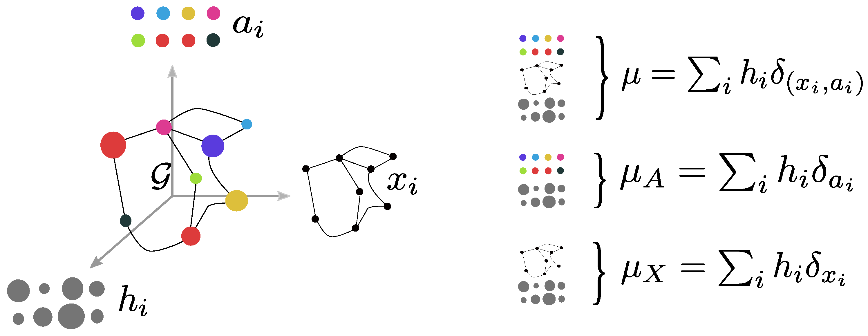
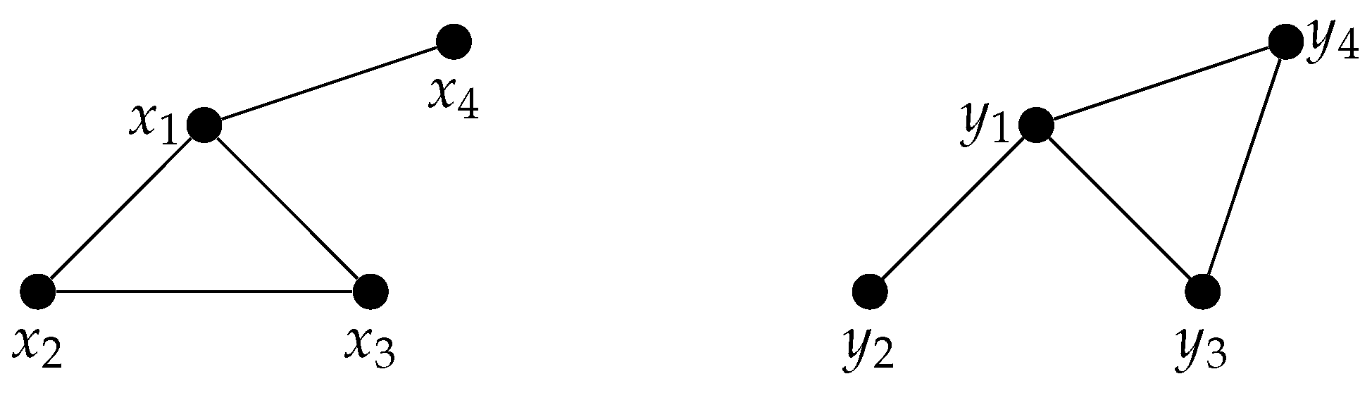
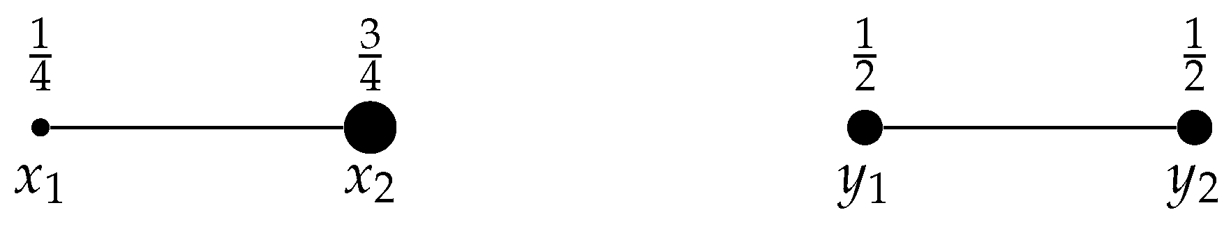
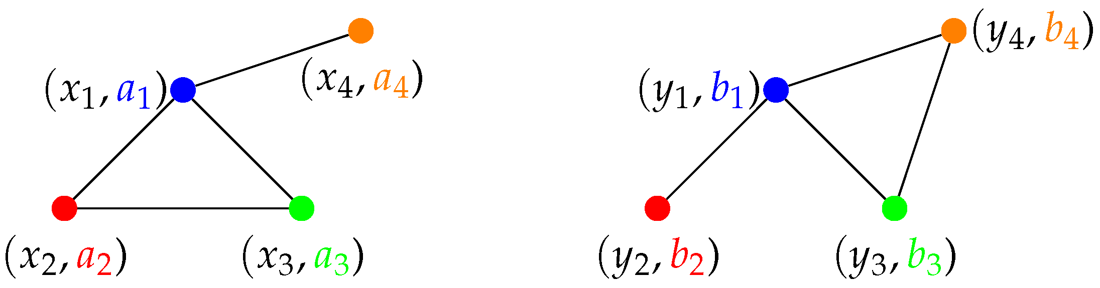
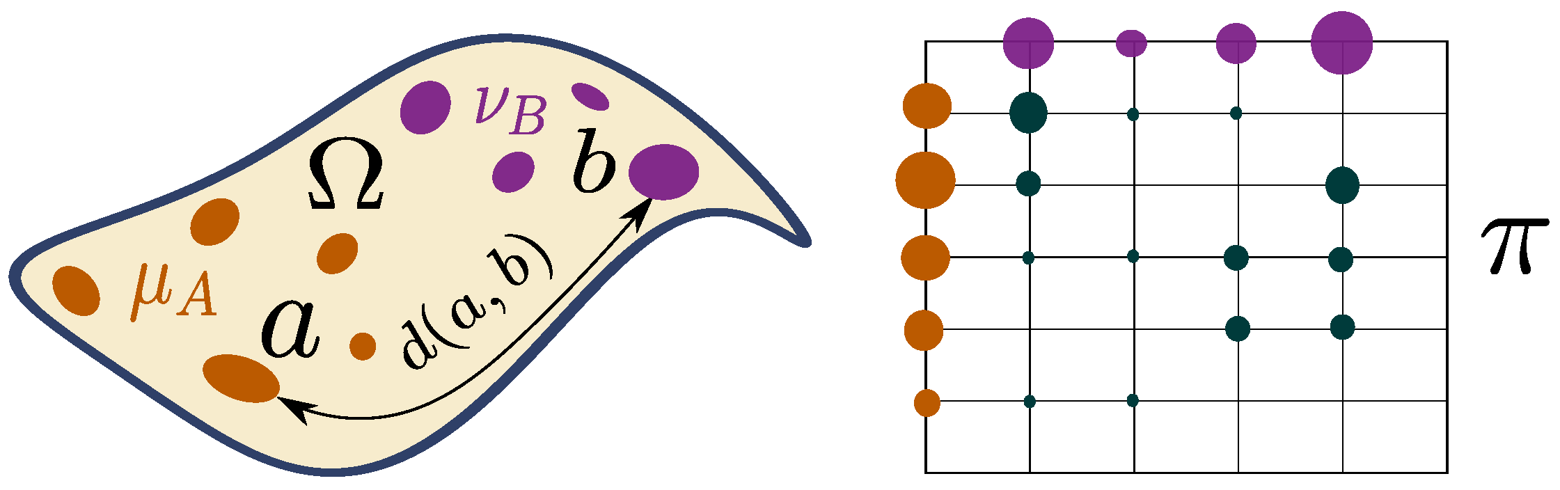
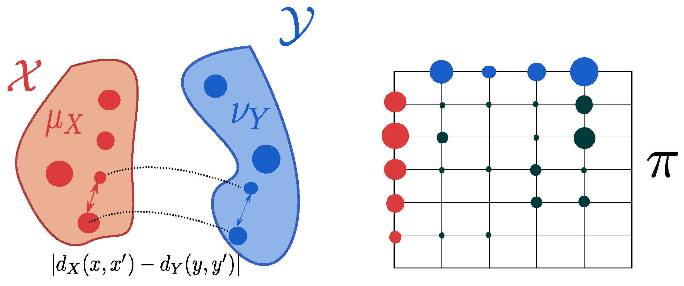
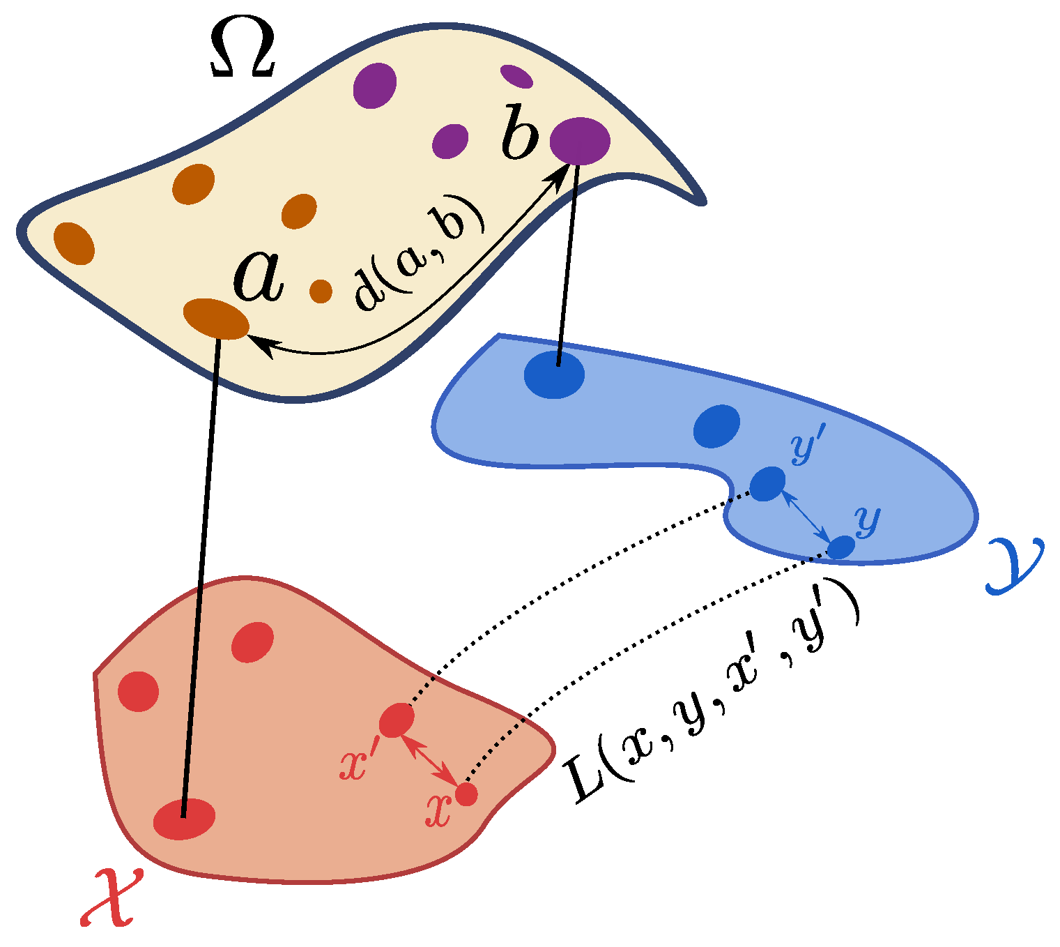
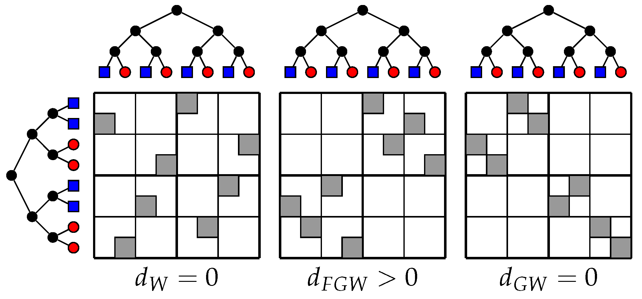
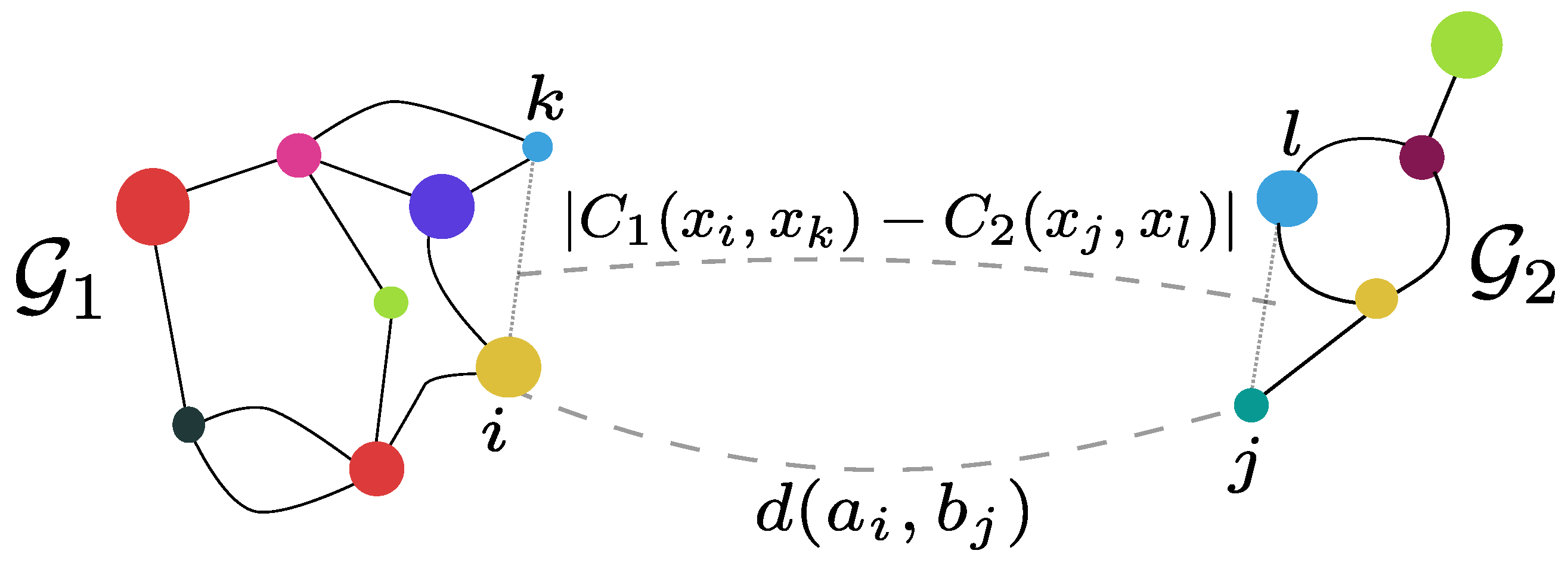
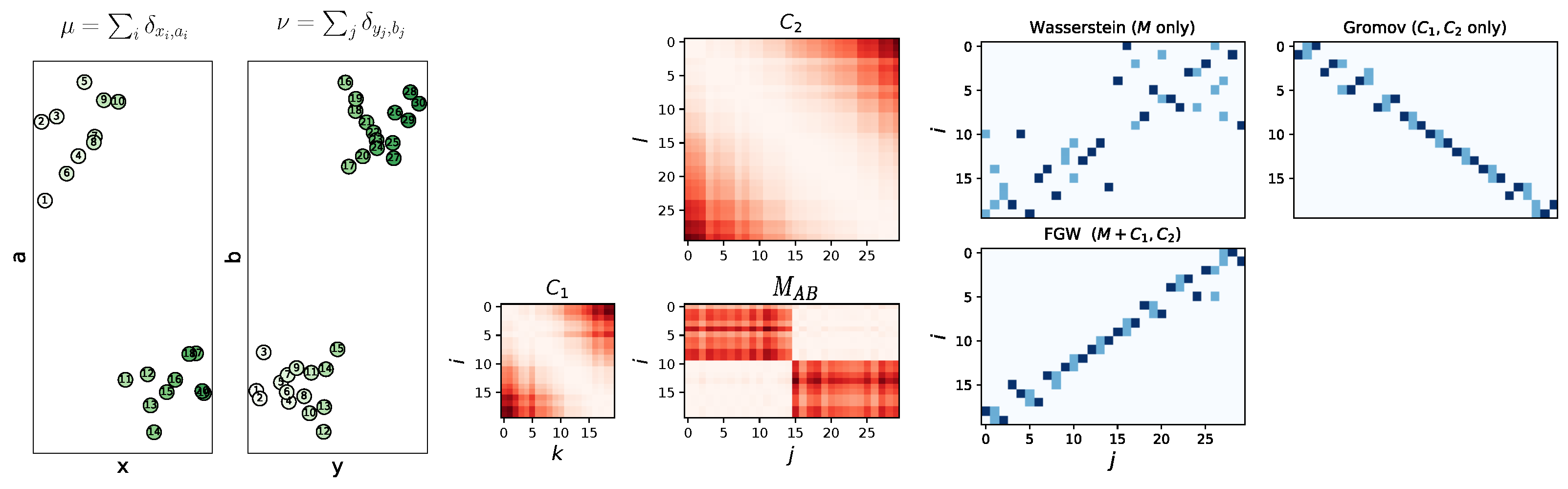
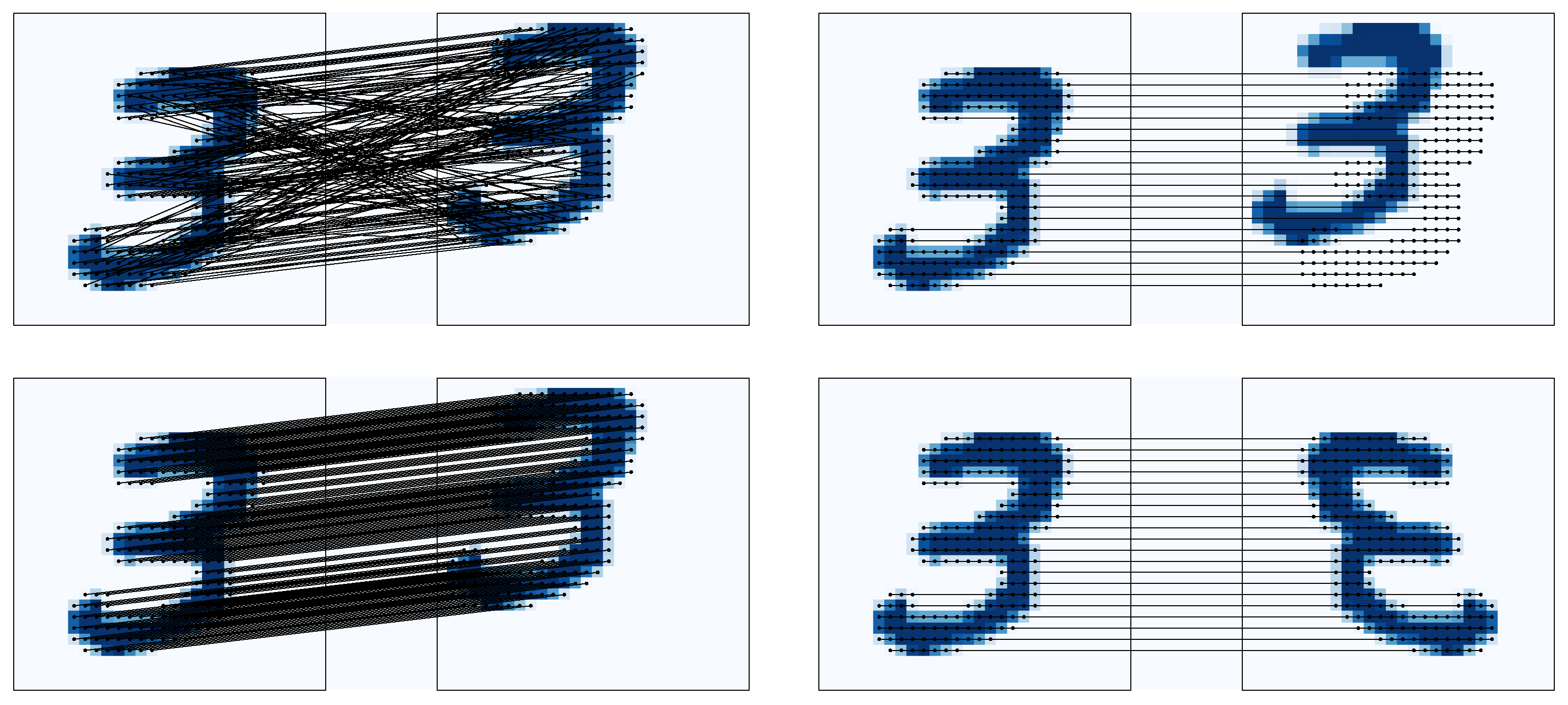
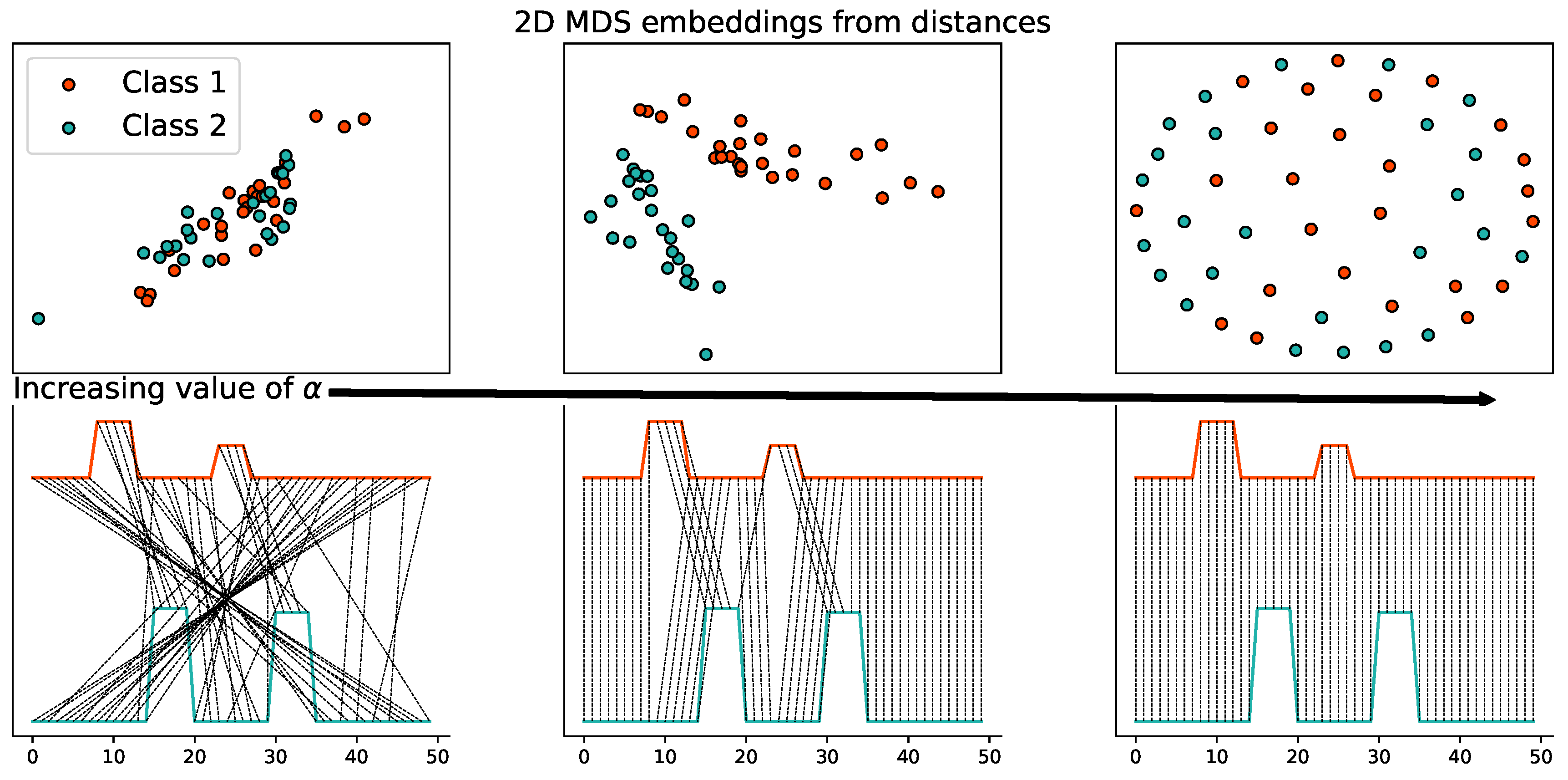
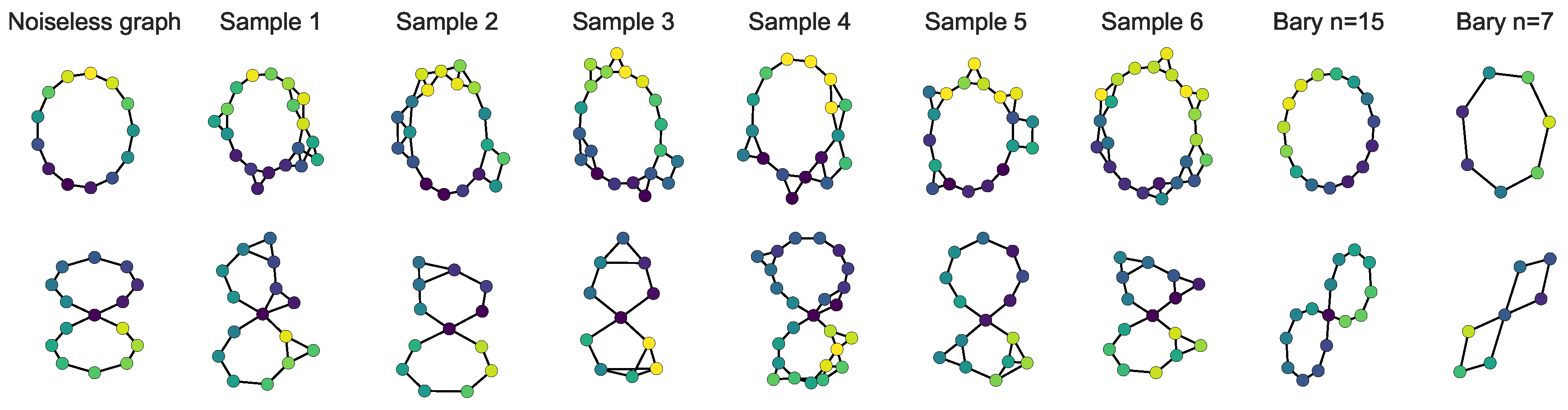
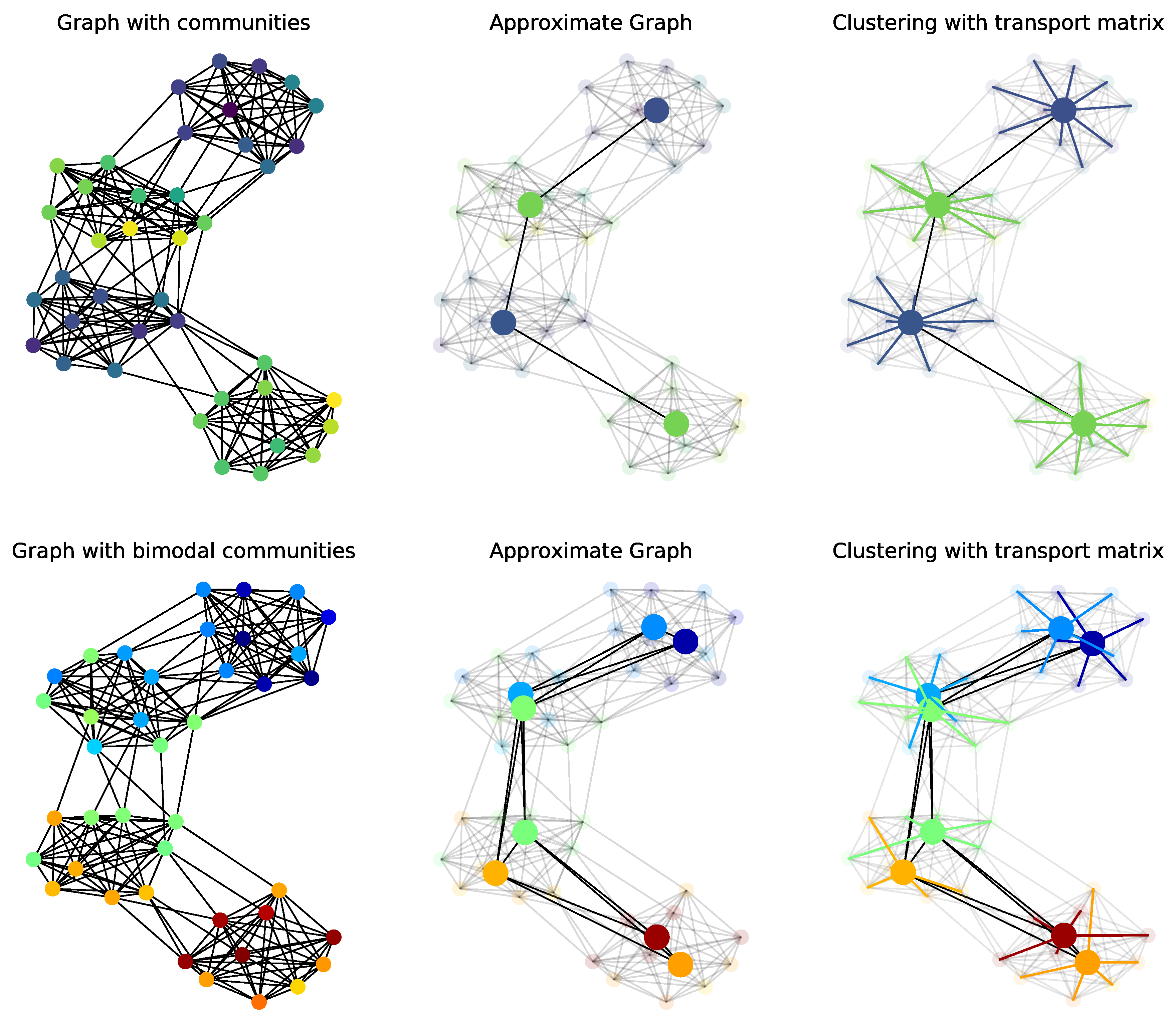
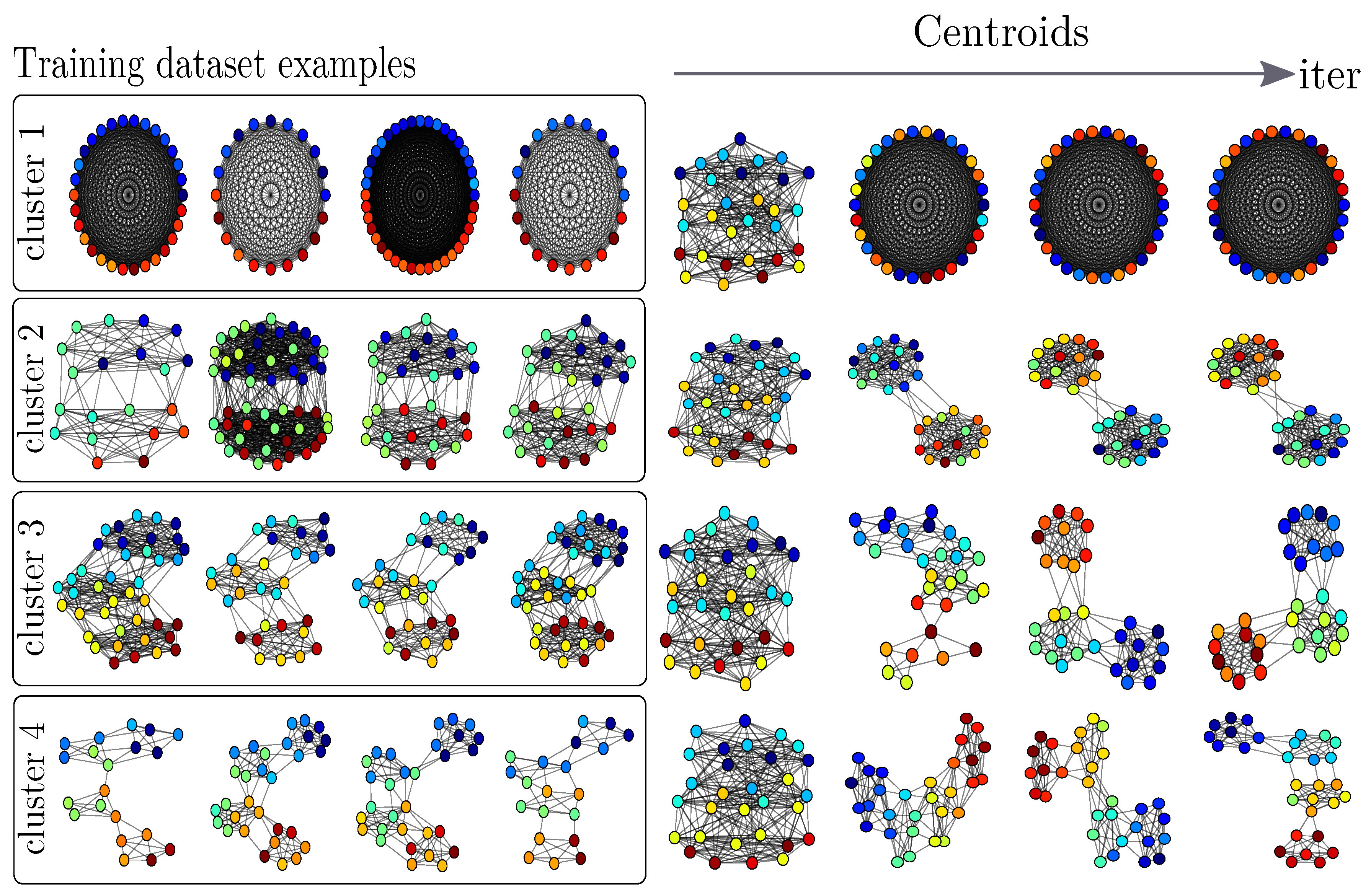
Table 1.
Average classification accuracy on the graph datasets with vector attributes.
| Vector Attributes | BZR | COX2 | CUNEIFORM | ENZYMES | PROTEIN | SYNTHETIC |
|---|---|---|---|---|---|---|
| FGW sp | 85.12 ± 4.15 * | 77.23 ± 4.86 | 76.67 ± 7.04 | 71.00 ± 6.76 | 74.55 ± 2.74 | 100.00 ± 0.00 |
| HOPPERK | 84.15 ± 5.26 | 79.57 ± 3.46 | 32.59 ± 8.73 | 45.33 ± 4.00 | 71.96 ± 3.22 | 90.67 ± 4.67 |
| PROPAK | 79.51 ± 5.02 | 77.66 ± 3.95 | 12.59 ± 6.67 | 71.67 ± 5.63 * | 61.34 ± 4.38 | 64.67 ± 6.70 |
| PSCN k = 10 | 80.00 ± 4.47 | 71.70 ± 3.57 | 25.19 ± 7.73 | 26.67 ± 4.77 | 67.95 ± 11.28 | 100.00 ± 0.00 |
| PSCN k = 5 | 82.20 ± 4.23 | 71.91 ± 3.40 | 24.81 ± 7.23 | 27.33 ± 4.16 | 71.79 ± 3.39 | 100.00 ± 0.00 |
Table 2.
Average classification accuracy on the graph datasets with discrete attributes.
| Discrete Attr. | MUTAG | NCI1 | PTC-MR |
|---|---|---|---|
| FGW raw sp | 83.26 ± 10.30 | 72.82 ± 1.46 | 55.71 ± 6.74 |
| FGW wl h = 2 sp | 86.42 ± 7.81 | 85.82 ± 1.16 | 63.20 ± 7.68 |
| FGW wl h = 4 sp | 88.42 ± 5.67 | 86.42 ± 1.63 | 65.31 ± 7.90 |
| GK k = 3 | 82.42 ± 8.40 | 60.78 ± 2.48 | 56.46 ± 8.03 |
| RWK | 79.47 ± 8.17 | 58.63 ± 2.44 | 55.09 ± 7.34 |
| SPK | 82.95 ± 8.19 | 74.26 ± 1.53 | 60.05 ± 7.39 |
| WLK | 86.21 ± 8.48 | 85.77 ± 1.07 | 62.86 ± 7.23 |
| WLK h=2 | 86.21 ± 8.15 | 81.85 ± 2.28 | 61.60 ± 8.14 |
| WLK h = 4 | 83.68 ± 9.13 | 85.13 ± 1.61 | 62.17 ± 7.80 |
| PSCN k = 10 | 83.47 ± 10.26 | 70.65 ± 2.58 | 58.34 ± 7.71 |
| PSCN k = 5 | 83.05 ± 10.80 | 69.85 ± 1.79 | 55.37 ± 8.28 |
Table 3.
Average classification accuracy on the graph datasets with no attributes.
| Without Attribute | IMDB-B | IMDB-M |
|---|---|---|
| GW sp | 63.80 ± 3.49 | 48.00 ± 3.22 |
| GK k = 3 | 56.00 ± 3.61 | 41.13 ± 4.68 |
| SPK | 55.80 ± 2.93 | 38.93 ± 5.12 |
© 2020 by the authors. Licensee MDPI, Basel, Switzerland. This article is an open access article distributed under the terms and conditions of the Creative Commons Attribution (CC BY) license (http://creativecommons.org/licenses/by/4.0/).
Share and Cite
MDPI and ACS Style
Vayer, T.; Chapel, L.; Flamary, R.; Tavenard, R.; Courty, N. Fused Gromov-Wasserstein Distance for Structured Objects. Algorithms 2020, 13, 212. https://0-doi-org.brum.beds.ac.uk/10.3390/a13090212
AMA Style
Vayer T, Chapel L, Flamary R, Tavenard R, Courty N. Fused Gromov-Wasserstein Distance for Structured Objects. Algorithms. 2020; 13(9):212. https://0-doi-org.brum.beds.ac.uk/10.3390/a13090212
Chicago/Turabian StyleVayer, Titouan, Laetitia Chapel, Remi Flamary, Romain Tavenard, and Nicolas Courty. 2020. "Fused Gromov-Wasserstein Distance for Structured Objects" Algorithms 13, no. 9: 212. https://0-doi-org.brum.beds.ac.uk/10.3390/a13090212
Note that from the first issue of 2016, this journal uses article numbers instead of page numbers. See further details here.