A Two-Phase Approach for Semi-Supervised Feature Selection
by
 , , ,
, , ,
Amit Saxena
1, 
Shreya Pare
2,
Mahendra Singh Meena
2,
Deepak Gupta
3 ,
,
Akshansh Gupta
4,
Imran Razzak
5,
Chin-Teng Lin
2 and
Mukesh Prasad
2,* 1
Department of Computer Science and Information Technology, Guru Ghasidas University, Bilaspur, Chhattisgarh 495009, India
2
School of Computer Science, FEIT, University of Technology Sydney, Sydney, NSW 2007, Australia
3
Department of Computer Science & Engineering, National Institute of Technology Arunachal Pradesh, Yupia 791112, India
4
Central Electronics Engineering Research Institute, Delhi 110028, India
5
School of Information Technology, Deakin University, Geeloing, VIC 3217, Australia
*
Author to whom correspondence should be addressed.
Algorithms 2020, 13(9), 215; https://0-doi-org.brum.beds.ac.uk/10.3390/a13090215
Submission received: 19 July 2020
/
Revised: 19 August 2020
/
Accepted: 25 August 2020
/
Published: 31 August 2020
Abstract
:This paper proposes a novel approach for selecting a subset of features in semi-supervised datasets where only some of the patterns are labeled. The whole process is completed in two phases. In the first phase, i.e., Phase-I, the whole dataset is divided into two parts: The first part, which contains labeled patterns, and the second part, which contains unlabeled patterns. In the first part, a small number of features are identified using well-known maximum relevance (from first part) and minimum redundancy (whole dataset) based feature selection approaches using the correlation coefficient. The subset of features from the identified set of features, which produces a high classification accuracy using any supervised classifier from labeled patterns, is selected for later processing. In the second phase, i.e., Phase-II, the patterns belonging to the first and second part are clustered separately into the available number of classes of the dataset. In the clusters of the first part, take the majority of patterns belonging to a cluster as the class for that cluster, which is given already. Form the pairs of cluster centroids made in the first and second part. The centroid of the second part nearest to a centroid of the first part will be paired. As the class of the first centroid is known, the same class can be assigned to the centroid of the cluster of the second part, which is unknown. The actual class of the patterns if known for the second part of the dataset can be used to test the classification accuracy of patterns in the second part. The proposed two-phase approach performs well in terms of classification accuracy and number of features selected on the given benchmarked datasets.
1. Introduction
Pattern classification [1] is one of the core challenging tasks [2,3] in data mining [4,5], web mining [6], bioinformatics [7], and financial forecasting [8,9]. The goal of classification [10,11] is to assign a new entity to a class from a pre-specified set of classes. As a particular case, the importance of pattern classification can be realized in the classification of breast cancer. There are two classes of patients, one belonging to the “benign” class, having no breast cancer, while the other class of patients belong to the “malignant” class, which shows strong evidence of breast cancer. A good classifier will reduce the uncertainty of misclassifying patients from being in one of these two classes. Recently, a novel approach was presented using a real-coded genetic algorithm (GA) for a polynomial neural network classifier (PNN) [12]. The polynomials have powerful approximation properties [13] and excellent properties as a classifier [12].
One of the major problems in the mining of large databases is the dimension of the data. More often than not, it is observed that some features do not affect the performance of a classifier. There could be features that are derogatory in nature and degrade the performance of classifiers. Thus, one can have redundant features, bad features, and highly correlated features. Removing such features can not only improve the performance of the system but also make the learning task much simpler. More specifically, the performance of a classifier depends on several factors: (i) number of training instances; (ii) dimensionality, i.e., number of features; and (iii) complexity of the classifier.
Dimensionality reduction can be done mainly in two ways: selecting a small but important subset of features and generating (extracting) lower-dimensional data, preserving the distinguishing characteristics of the original higher-dimensional data [14]. Dimensionality reduction not only helps in the design of a classifier, but also helps in other exploratory data analysis, assessment of clustering tendency, as well as to decide on the number of clusters by looking at the scatterplot of the lower-dimensional data. Feature extraction and data projection can be viewed as an implicit or explicit mapping from a p-dimensional input space to a q (p ≥ q)-dimensional output space such that some criterion is optimized.
A large number of approaches for feature extraction and data projection are available in the pattern recognition literature [15,16,17,18,19,20]. These approaches differ from each other in terms of the nature of the mapping function, how it is learned, and what optimization criterion is used. Feature selection leads to savings in measurement cost, because some of the features get discarded. Another advantage of selection is that the selected features retain their original interpretation, which is important to understand the underlying process that generates the data. On the other hand, extracted features sometimes have better discriminating capability, leading to better performance, but these new features may not have any clear physical meaning.
When feature selection methods use class information, it is called supervised feature selection. Although the majority of the feature selection methods are supervised in nature, there has been a substantial amount of work using unsupervised methods [21,22,23,24,25,26,27,28]. Apart from supervised and unsupervised feature selection where classes are known and unknown, respectively, one more category of datasets is available called semi-supervised, where the classes are assigned to some of the patterns only. The methods to classify unknown patterns come under the category of semi-supervised methods, and feature selection on such datasets is called semi-supervised feature selection.
The contributions of the paper are as follows:
- i.
- To find a subset of features that has maximum relevance and minimum redundancy (abbreviated to MRmr herein) by using the correlation coefficient. For this purpose, an algorithm (Algorithm 1) is presented to maintain a balance between the features with high relevance and the features with minimum redundancy.
- ii.
- To determine a small feature subset that produces high classification accuracy on a supervised classifier to minimize time and complexity of implementing the method.
- iii.
- The proposed method aims to demonstrate the idea that if we have a pair of two clusters that are almost identical or much closer to each other, if we know the class of a cluster of the pair, the same class can be assigned to the other cluster of the pair.
- iv.
- The class or labels of all patterns can be determined using the proposed novel approach, which will save time or cost in collecting patterns for each pattern in the dataset otherwise.
- v.
- The proposed method is a novel concept and can be applied to various real datasets.
This paper is organized as follows: The existing techniques of feature selection are presented in Section 2. Section 3 presents preliminaries of the methods used in the paper. Section 4 presents the proposed scheme with two algorithms. The experiments are presented in Section 5. The results obtained from the proposed approach after experiments are discussed in Section 6 followed by conclusions in Section 7.
2. Existing Feature Selection Techniques
The problem of feature selection can be formulated as follows: Given a dataset (i.e., each has p features), we have to select a subset of features of size q that leads to the smallest (or highest as the case may be) value with respect to some criterion. Let Ƒ be the given set of features and F the selected set of features of cardinality m, FƑ. Let the feature selection criterion for the dataset X be represented by J(F, X) (lower value of J(.) indicates a better selection). When the training instances are labeled, we can use the label information, but in the case of unlabeled data, this cannot be done [29].
In Saxena et al. [29], a new approach to unsupervised feature selection preserving the topology of the data is proposed. Here, the genetic algorithm (GA) has been used to select a subset of features by taking the Sammon stress/error as the fitness function. The dataset with the reduced set of features is then evaluated using classification (1–nearest neighbor (1–NN)) and clustering (K-means) techniques. The correlation coefficient between the proximity matrices of the original dataset and the reduced one is also computed to check how well-preserved the topology of the dataset is in the reduced dimension. In feature selection, the filter model [30,31,32], wrapper model [33], and embedded model [34] are three main categories. The filter model relies on the features’ properties with certain evaluation metrics. In the wrapper model, it evaluates feature sets via the model’s prediction accuracy with a combination of features. For the embedded model, the feature selection part and the learning part interact with each other. Though the wrapper model and embedded model can achieve effectively selected features in certain cases, the computational cost is high in application [35].
Supervised feature selection relies on the classification labels, and the typical models are the Fisher metric [36] and Pearson’s correlation coefficient [37]. Unsupervised feature selection is based on feature similarity or local information. Laplacian score [38] is a typical unsupervised feature selection model, which measures the geometrical properties in the feature sets. Utilizing both the labeled data and unlabeled data is a method to achieve optimal feature subsets, which is the focus of semi-supervised feature selection [39]. In [40], both labeled and unlabeled data are trained via the spectral analysis to establish a regularization framework, and the authors demonstrate that the unlabeled data can be helpful for feature selection. In [41], label propagation is conducted and a wrapper-type forward semi-supervised feature selection framework is proposed.
Xu et al. in [35] used Pearson’s correlation coefficients to measure the feature-to-feature, as well as the feature-to-label, information. The coefficients are trained with the labeled and the unlabeled data, and the combination of this two-fold information is performed with max-relevance and min-redundancy criteria. The experiments are applied on several real-life applications [35]. Despite having labeled or unlabeled datasets individually, it is natural to have a mix of both, viz. labeled and unlabeled, in a single dataset. Such types of semi-supervised datasets can be made available intentionally or unintentionally. For the former case, labeling datasets may cost a large amount due to the processes involved to obtain labels after several experiments. In the latter case, labels are missing or doubtful or as good as not available. Some literature can be seen in Sheikhpour [42]. In this paper, we propose a two-phase approach to find the missing labels of patterns of a dataset that contains some labeled data (patterns).
3. Preliminaries of the Methods Used in the Proposed Approach
The basics of some methods used in this paper are outlined below for a quick reference.
Classification: The process of separating data into groups based on some given labels or similarities. Much has been described before. In supervised classification, the training data contain the labels; the knowledge of these labels will be used to determine the label of the testing data.
Clustering: When the labels are not tagged with the patterns in advance. Similarity among the patterns is used to group (cluster) the datasets. A common approach is to start with a random set of centroids (some or all of them can even be taken as different existing patterns of the dataset),which represent their respective clusters, and then bring the closest patterns (i.e., nearest to the centroid) in a cluster. After a repetitive exercise, we obtain a set of centroids such that the patterns belonging to the clusters represented by these centroids do not shift from one cluster to the other even after repeating the exercise further. This approach is known commonly as K-means clustering [43]. The K-means algorithm has some defects: (1) Algorithm is sensitive to the initial cluster center. The selection of initial centers of the pros and cons will affect the clustering results, and then influence the efficiency of the algorithm performance; (2) the algorithm is sensitive to outlier data and will result in a local optimal solution [44].
Fuzzy C-Means (FCM): FCM is a clustering method that allows one point to belong to two or more clusters, unlike K-means where only one cluster is assigned to each point. This method was developed by Dunn in 1973 [45] and improved by Bezdek in 1981 [46]. The FCM provides a broader and soft assignment of a point to a cluster, which is why it is preferred over K-means. For more detail about the clustering techniques, refer to the article by Saxena et al. [47]. Some semi-supervised FCM clustering algorithms are available in the literature; for an overview, refer to [48]. Garibaldi et al. [49] proposed an algorithm where they apply an effective feature enhancement procedure to the entire dataset to obtain a single set of features or weights by weighting and discriminating the information provided by the user. By taking pair-wise constraints into account, they proposed a semi-supervised fuzzy clustering algorithm with feature discrimination (SFFD) incorporating a fully adaptive distance function. Although there can be other methods for semi-supervised feature selection, the objective of the present work is to apply a mechanism to obtain a subset of influential features with MRmr in Phase-1. Then, the reduced dataset due to the presence of only influential features will be clustered. In Phase-2, clustering of the reduced dataset is required and, for this purpose only, any clustering algorithm could be applied. For its flexibility in deciding a pattern for affiliation to a cluster (against K-means clustering), the FCM has been used.
Correlation: These methods are used to find a relationship among attributes (or columns) in a dataset. The most common method to determine the correlation between two column vectors is achieved by computing Pearson’s correlation (RRPC) coefficient. For any two column vectors X and Y, Pearson’s correlation coefficient is calculated as follows:
where xi and yi are the i-th values of the two feature vectors X and Y with their means as x– and y–, respectively. When the value of is close to 1 (one), the two constituent column vectors are said to be highly correlated. On the other hand, closeto 0 (zero) indicates a very poor or no similarity between the two vectors.
Polynomial Neural Networks (PNNs): PNNs are a flexible neural architecture in which the topology is not predetermined or fixed, as in a conventional artificial neural network (ANN) [50], but is grown through learning layer by layer. The design is based on the group method of data handling (GMDH), which was invented by Ivakhnenko [51,52]. Ivakhnenko developed the GMDH as a means of identifying nonlinear relations between input and output variables. The individual terms generated in the layers are partial descriptions (PDs) of data, being the quadratic regression polynomials with two inputs [12].
PNN-based methods used for comparison in this paper are as follows:
- P1: Simple PNN method: The inputs fed in the input layer generate PDs in the successive layers [53].
- P2: RCPNN with gradient descent [53]: A reduced and comprehensible polynomial neural network (RCPNN) model generates PDs for the first layer of the basic PNN model, and the outputs of these PDs along with the inputs are fed to the single-layer feed-forward neural network. The network has been trained using gradient descent.
- P3: RCPNN with particle swarm optimization (PSO): This method is the same as the RCPNN except that the network is trained using particle swarm optimization (PSO) [54] instead of the gradient descent technique.
- P4: Condensed PNN with swarm intelligence: In this paper, Dehuri et al. [55] proposed a condensed polynomial neural network using swarm intelligence for the classification task. The model generates PDs for a single layer of the basic PNN model. Discrete PSO (DPSO) selects the optimal set of PDs and input features, which are fed to the hidden layer. Further, the model optimizes the weight vectors using the continuous PSO (CPSO)technique [55].
- P5: All PDs with 50% training used in the proposed scheme of [12].
- P6: All PDs with 80% training used in the proposed scheme of [12].
- P7: Only the best 50% PDs with 50% training used in the proposed scheme of [12].
- P8: Only the best 50% PDs with 80% training used in the proposed scheme of [12].
- P9: Saxena et al. [29] proposed four methods for feature selection in an unsupervised manner by using the GA. The proposed methods also preserve the topology of the dataset despite reducing redundant features.
A brief summary of methods P5–P8 as used by Lin et al. [12]: In this work [12], a real-coded genetic algorithm (RCGA) has been used to improve the performance of a PNN. The PNN tends to expand to a large number of nodes, which results in a large computation, making it costly in terms of time and memory. In this approach, the partial descriptions are generated at the first layer based on all possible combinations of two features of the training input patterns of a dataset. The set of partial descriptions from the first layer, the set of all input features, and a bias constitute the chromosome of the RCGA. The ability to solve a system of equations is utilized to determine the values of the real coefficients of each chromosome of the real-coded genetic algorithm for the training dataset with the mean classification accuracy (abbreviated to CA herein) as the fitness measure of each chromosome. To adjust these values for unknown testing patterns, the RCGA is iterated using selection, crossover, mutation, and elitism.
4. Proposed Two-Phase Approach
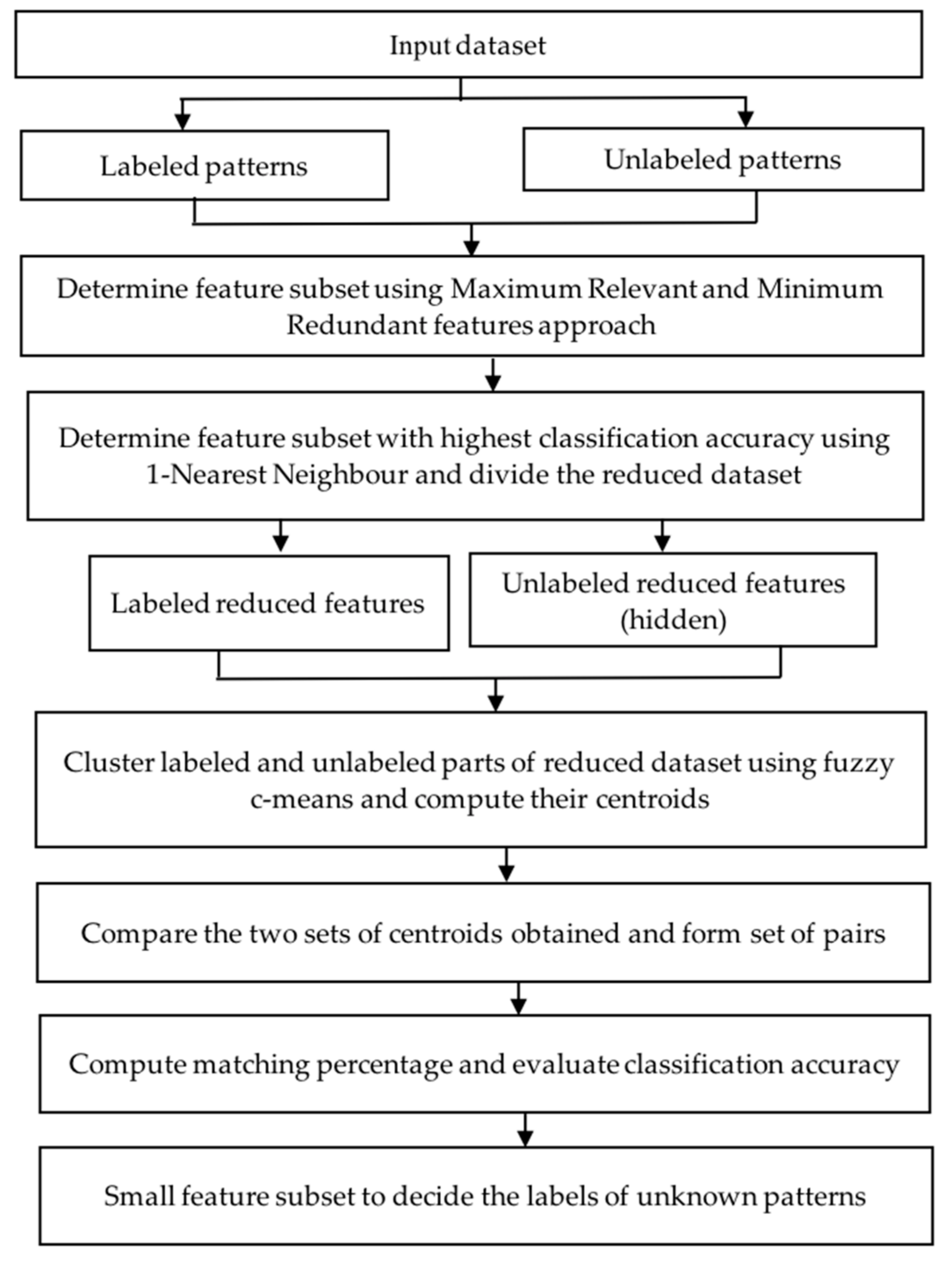
The proposed approach includes two algorithms with some assumptions given in this section. The flow diagram of the proposed approach is given in Figure 1.
4.1. Assumptions
The dataset used for simulation purpose contains some patterns that have labels (or class) while the remaining patterns do not contain labels. It is also assumed that all the possible available classes have been included in the part of the dataset with known classes. In other words, no new class is assumed to be possessed by any unlabeled pattern. Here, it is to clarify that for the performance measure, we take datasets where all patterns are labeled but hide classes of some of the patterns and assume these are unlabeled patterns. If we partition the datasets into a given number of clusters, each cluster shows at least one of the classes in the majority, and that class will represent that cluster. For this reason, we calculate the majority of patterns belonging to a particular class in a cluster, and that cluster will be labeled with that class. The description of datasets is given in Table 1. The number of patterns with known and unknown labels in the dataset is given in Table 2.
4.2. Algorithm of the Two-Phase Approach
Phase-I: Finding the reduced number of features (feature selection) and then finding the centroids of the clusters in the reduced dataset where classes are known.
Phase-II: Determining the classes of patterns of the other part of the reduced dataset where classes are unknown with the help of their closest clusters obtained in the first part.
The overall steps involved in the proposed two phase approach are presented in the Algorithm 2. The steps for calculating the maximum relevant and minimum redundant features are shown in Algorithm 1. The details of Algorithms 1 and 2 are given below:
| Algorithm 1 The maximum relevant and minimum redundant features |
Input: Dataset with d features; with labels given on some patterns (supervised) and not given on some patterns (unsupervised)
|
| Algorithm 2 The steps of the proposed two-phase approach |
|
As an example, take wine data, which has 13 features. Now, according to Table 3, 50% of 13 when rounded equals 7. Thus, by step 2 of Algorithm 1, seven sorted features (in descending order of the values of correlation coefficients) are found as F_Sup_red = {4,8,2,10,3,5,1}. Similarly for the unsupervised case, mentioned in Step 4 of Algorithm 1 above, seven combinations of features (in ascending order of the values of correlation coefficients) are obtained as F_UnSup_red = {(2,11),(7,8),(10,11),(8,12),(6,8),(4,13),(10,12)}. According to Step 5 of Algorithm 1, the poorest feature subset will contain those features that belong to F_UnSup_red but do not belong to F_Sup_red, i.e., F_poorest = {6,7,11,12,13}. Now, calculate F_best as an intersection of subsets of F_Sup_red = {4,8,2,10,3,5,1} and F_UnSup_red = {(2,11),(7,8),(10,11),(8,12),(6,8),(4,13),(10,12)}. Therefore, F_best is computed as {2,4,8,10}, which gives a cardinality of 4. Now, form combinations of four features from F_Sup_red, i.e., {4,8,2,10,3,5,1}, 7C4, which is 35. Thus, 35 combinations will be formed, each combination having four features from {4,8,2,10,3,5,1}. The feature subset {1,2,3,10} produced the highest CA when labels of 70% patterns were known; therefore, this subset was chosen. Similarly, for 50% and 40% of the known labels, feature subset {1,2,8,10} was chosen as it produced the highest CA in both cases.
As another example consider Wisconsin Breast Cancer (WBC) data that have nine features. Now, according to Table 3, 50% of 9 when rounded equals to 5. Thus, by step 2 of Algorithm 1 above, five sorted features (in descending order of the values of correlation coefficients) are found as F_Sup_red = {2,3,6,7,8}. Similarly, for unsupervised case, mentioned in Step 4 of Algorithm 1 above, five combinations of features (in ascending order of the values of correlation coefficients) are obtained as F_UnSup_red = {(6,9),(7,9),(1,9),(4,9),(8,9)}. According to Step 5 of Algorithm 1, the poorest feature subset will contain those features that are in F_UnSup_red but not in F_Sup_red, i.e., F_poorest = {1,4,9}. Now, calculate F_best as an intersection of subsets of F_Sup_red = {2,3,6,7,8} and F_UnSup_red = {(6,9),(7,9),(1,9),(4,9),(8,9)}. Therefore, F_best is computed as {6,7,8}, which gives a cardinality of 3. Now, form combinations of three features from F_Sup_red, i.e., {2,3,6,7,8}, 5C3, which is 10. Thus, 10 combinations will be formed, each combination having three features from {2,3,6,7,8}. The feature subset {3,6,8} produced the highest CA when labels of 70% patterns were known; therefore, this subset was chosen. Similarly, for 50% known labels, subset {2,6,8}, and for patterns having 40% known labels, feature subset {3,6,7} were chosen as these subsets produced the highest CA. The pseudo code of the proposed two-phase approach is as below:
| Pseudo-Code: The proposed two-phase approach |
Input DF,P dataset with F features, P number instances and number of classes as C
|
4.3. Complexity of Algorithms
Xu et al. [35] proposed an RRPC-based Semi-Supervised Feature Selection Approach. The criteria used maximum relevance while selecting features for supervised learning and minimum redundancy for unsupervised learning of features. The criterion is incremental in nature as the features are added one by one. The approach used in this paper also applies relevancy and redundancy criteria for determining an optimum set of features on the basis of values of correlation coefficients. The selection of an optimum subset of features is given in Algorithm 1. The emphasis in the paper is to maintain a good composition of features having high relevancy but minimum redundancy. The features with minimum values of correlation coefficients have been dropped if they are not part of those features that have high relevancy. An advantage of the present method is that it is simple and easy to implement. It is a new but efficient approach as well. There is no incremental approach used in this paper. All the features are pre-allocated in the dataset. Another advantage is the application of knowledge about clusters. This concept is probably not reflected in the literature to the best of our perception. In a dataset, training data can be divided into clusters with some centroids (K, for instance). The test data are also clustered with some centroids. The dataset is the same, so the clusters must also match in both partitions, i.e., training data as well as testing data. The ordering of a point in a centroid can be in a different order, but a centroid in the training data that is nearest to a centroid in the testing data must match. Therefore, the label attached to the cluster in the training data must be same as its closed centroid in the test data.
The computational complexity of the present two-phase algorithm is a sum of the following factors:
- i.
- Calculating Pearson’s Coefficient O(n)
- ii.
- Calculating Fuzzy C-means clustering O(ndc2i)
- iii.
- Time for calculating KNNO(ndK).
Sum O(n(1 + d(c2i + 1)); K = 1 as in this work, and 1–Nearest Neighbor is used, where n is the number of observations (patterns) in the dataset under process, d is the number of features (attributes), c is the number of clusters (classes or labels),and i is the number of iterations. In RRPC proposed by Xu et al. [35], the computational complexity is given by the sum of terms (a) due to the similarity of matrices: O(l(d + 1)2 + ud2), and (b) due to feature ranking: O(n(d + 1)2 + nd2); hence, total complexity = a + b; where l + u = n. l: Labeled and u: Unlabeled patterns.
5. Experiments
The proposed two-phase method was run on an i5 machine using MATLAB. The semi-supervised dataset was considered to contain two types of patterns: One part that contains the labels and the other part that does not contain labels. For finding the reduced number of features in the whole dataset, we used the approach proposed by Xu et al. [35] and used the Karl Pearson Correlation coefficient method with MRmr. For obtaining a feature subset with MRmr, Algorithm 1 is applied. Form all combinations of features from the feature set as mentioned in Algorithm 1. Find out the CA with every combination of the reduced set of features formed as above by the 1–NN method. Find out the feature subset that provides maximum CA. Thus, we have a reduced set of features; transform the whole dataset with the reduced number of features. Divide the reduced dataset into two parts: One part that contains class labels and the other part where the class labels are kept hidden. This completes Phase-I of the proposed approach. Prior to beginning Phase-II, apply any clustering algorithm (K-means clustering in present work) to divide the reduced dataset obtained in the first part into the number of clusters that is the same as the number of available classes used in the first part. Now, collect the centroids (equal to the number of classes in the first part). If we have c classes and r reduced number of features, we obtain c cluster centroids (rows) and each centroid has r values (columns). In each cluster, the class attached to the majority of patterns will be considered as the class of that cluster. This is verified by several experiments used in this method.
Phase-II starts with the second part of the reduced dataset, which is unsupervised; no classes are known. Divide this dataset into a number of clusters that is the same as the number of available classes of the dataset. Find out the centroids of the obtained clusters. Each cluster will contain a number of patterns with unknown class. Compare these centroids to those obtained in the first part of Phase-1. Find out a good mapping of each centroid in the second part with that obtained in the first part. Form the pairs of clusters such that each pair contains the first cluster centroid from the first part and the second cluster centroid from the second part of the dataset. As the class of the first cluster of this pair is known, as mentioned in Phase-I, the same class will be assigned to the second cluster belonging to the second part. The second part is already clustered in the beginning and the class of each cluster of the second part is also decided using this approach. Therefore, each pattern belonging to the clusters of the second part of the dataset will be the same as the class tagged with the individual clusters decided before. For verification, we check the class of each pattern of clusters of the second part with the original dataset. The accuracy of the matching of patterns is computed. In this manner, we also find the class of the second part, which was unknown originally.
Methods Used: For classification, we used 1–NN in Phase-I. The Karl Pearson Coefficient was used to find relevance and redundancy. Fuzzy C-means clustering [46] was used to divide datasets into C clusters. C was also used as the number of available classes. The summaries of these methods are presented in Section 3.
We used nine datasets summarized in Table 1. The datasets are divided into two parts. The ratios of known (labeled) classes against unknown classes (unlabeled), with the number of patterns in percent, are given in Table 2. The size of feature subsets to be used for processing is given in Table 3. The correlation coefficient values for a typical dataset (WBC) are given in Table 4 and Table 5 for relevance and redundancy purposes, respectively. In Table 4, as well as in Table 5, the set of features selected are also given based on higher and lower correlation coefficient values, respectively. The features that are considered good in Table 4 with high correlation coefficient values must be retained in the final feature set, whereas the features having low correlation coefficient values must not find a place in the final feature set. Table 6 provides results obtained using the proposed two-phase method. Table 7 shows distances between centroids obtained by the second-part and first-part clusters. Table 8 presents a comparison of CA values obtained by various methods reported in the literature. Table 9 presents a list of features used by various methods for processing.
The methods P1–P9 are summarized in Section 3.
- *P1–Basic PNN
- *P2–RCPNN with gradient descent
- *P3–RCPNN with PSO
- *P4–Condensed PNN with swarm intelligence
- *P5–All PDs with 50% training in proposed scheme
- *P6–All PDs with 80% training in proposed scheme
- *P7–Only best 50% PDs with 50% training in proposed scheme
- *P8–Only best 50% PDs with 80% training in proposed scheme
- *P9–Unsupervised method using Sammon’s Stress Function
- *P10–Proposed method with 70% known labels
- *P11–Proposed method with 50% known labels
- *P12–Proposed method with 40% known labels
6. Results and Discussion
This paper proposes a two-phase method to find out the most probable labels attached to some of the patterns in a dataset. The main concept is to utilize the knowledge of the patterns in the dataset that are labeled. The results achieved from the experiments performed are shown in various tables. Table 1 presents the description of the datasets used for experiments. These benchmark datasets are collected from the UCI repository [56,57]. The synthetic data are used to verify the correctness of the method as it is obvious that the results for synthetic data would yield maximum accuracy. For all real datasets, various ratios of the number of labeled patterns vs. number of unlabeled patterns (shown in percent) are shown in Table 2. It is apparent from this table that all experiments have been performed on three sizes of datasets in terms of a known and unknown number of patterns: (70,30), (50,50), and (40,60). Table 6 presents results obtained from experiments with various parameters. Column 1 shows the name of the dataset. Column 2 indicates what percent of portion has been used with known labels in the dataset. This information is shown in Table 2. The correlation coefficients calculated as described in the proposed scheme in Section 3 are used to find out the number of features with maximum relevance for each dataset. In the third column, the features producing higher correlation coefficient values with the corresponding class labels are mentioned. These features are termed as features with maximum relevance in Table 6. Similarly, the fourth column shows the features with low redundancy based on minimum correlation coefficient values calculated by taking features together in pairs. These features are termed as features with minimum redundancy in Table 6. In other words, these features are considered harmful for classification purposes due to their redundant nature. Column 5 gives the list of features taken finally as a reduced subset. The dataset is reduced to this set of features. The CA obtained using 1–NN using the ratio, as shown in column 2, is listed in column 6 of this table. For the first part of the dataset with labeled patterns, Fuzzy C-means clustering is used to find out the centroids. These centroids are shown in Column 7 of the table. The centroids are also obtained for the remaining parts of the dataset with unlabeled patterns and shown in column 8. As explained in the description of the method before, pairs are made for each centroid of Column 7 with the centroid shown in Column 8. These pairs are given in Column 9. The class of each pattern in the second part (with unlabeled patterns) as described in the method is compared, and if it matches with the actual class assigned to that pattern, the number of matching patterns increases by 1. The percent of the matching patterns is shown in Column 10 of Table 6.
From Table 6, it is noted that for synthetic data, there are three features (1,2,3) that are found to have maximum relevance, whereas two features (4,5), albeit having minimum redundancy, have too poor a values and should, therefore, not be retained in the final feature subset. The final subset keeps only two features (1,2). The selection of the final feature set is as follows: Suppose we have five features in a dataset and decided to take only 50% of the total number of features on the high correlation coefficient values; thus, take the round of (5/2) = 3 features for which the correlation coefficient values between features and class are highest. Then, take those three features that have the lowest correlation coefficient values when the feature with other features are used to calculate correlation coefficient values. Now, take those features that are only in the former set and discard those in the latter set. Find a feature set with only there features. Again, reduce this feature to 50%. Round it so we obtain the round of (3/2) = 2. Thus, the final feature set will have only two features. Which two features will be retained in the final feature set is decided as follows. Find out the combination of two features (which should be in the final feature set) with all features in the feature set determined last having three features. We can have three sets of features, say, (1, 2), (2,3), and (1,3). Find out the CA with these three subsets of features of the dataset, and the feature set that gives the maximum CA will be used to provide the reduced feature set. The CA using features 1,2 in the dataset comes out to be 100% for each of the three ratios of datasets 70%,50%, and 40% of labeled data. Let us understand the centroid mapping at this stage using an example. For synthetic data, there are two features and two classes only. The first two rows in column 7 of the table indicate (1:5.06, 4.80; 2:19.60,19.61) the centroid value for cluster 1 and cluster 2, respectively. These centroids are calculated for the clusters that are obtained by partitioning the first part of the dataset where 70%, 50%, or 40% of the patterns are labeled. Similarly, in the next column, i.e., column 8 of Table 6, we have centroids for cluster 1 and cluster 2 as (1:5.00,4.78; 2:19.49,19.63), respectively. These centroids are computed from the second part of the dataset where labels are not given in the remaining 30%, 50%, and 60% of data. When we observe these two pairs of centroids, we find that the first centroid of cluster 2, (1:5.00,4.7), is much closer to the first centroid of cluster 1 (1:5.06,4.80). It is placed as (1,1), which means the first centroid of the unlabeled data cluster close to the first centroid of cluster 1 of the labeled data. Similarly, the pair (2,2) is obtained. As the second centroid in both cases (i.e., 2 in pair (2,2)) is labeled, the class of the first centroids of clusters 1 and 2 must also be same as their closed centroids in the labeled data. In this manner, each pattern of the unlabeled cluster is labeled one by one and simultaneously also compared to its original class. If the class of an unlabeled pattern using this method matches with the actual class assigned to it, the CA or the number of matching patterns increases by 1. We continue the exercise for all patterns in unlabeled clusters 1 and 2. After checking for all patterns, find the percent of matching patterns in the unlabeled part of the dataset that is shown in column 10 of Table 6. For synthetic data, it is 100%, meaning all patterns that were unlabeled are correctly labeled. The same exercise is repeated for all other datasets. For datasets where the number of features is up to 20, a maximum of half of the features are chosen either for maximum relevance or minimum redundancy level. For the datasets where the number of features is more than 20, we took only 10 higher values of correlation coefficients and 10 lower correlation coefficients only. The intersection of this set will give a refined feature set, and we take 50% of the features and repeat the exercise as above. Sonar and Ionos datasets are used with 60 and 34 features, respectively. While deciding the proximity of centroids with others, Euclidean distance was used to compute the distance. From the table, it is evident that for iris data, features 3 and 4 were chosen as good features, but only one feature (number 4) was taken in the final feature set. It reduces redundancy. Due to the random partitioning of the dataset, for 70% and 40% labeled data, feature 4 is chosen, whereas for 50% labeled data, feature number 3 is chosen as the best feature and with a CA of approximately 95%. After the clustering of labeled and unlabeled data and combining their centroids, the accuracy by predicting the class of unlabeled data is also high, nearly 95%. For the wine data where CA was 87–92% while selecting features for labeled data, the prediction accuracy by the proposed approach is 78–86% for the three folds of datasets. It is worth mentioning that every time we predict accuracy, at least 10 times the method was iterated so that we have proper validation of all parts of the datasets. The maximum values obtained out of these 10 iterations have been given in Table 6. Similarly, WBC data produce a prediction accuracy in the range of 96–98% after selecting features at an accuracy range of 96–97% approximately. The selection of feature subsets for wine and WBC data is explained in Section 3. Various values are similarly shown in this table. Liver data produce a lower prediction accuracy of 52–58% with a CA of 56–63% at the time of reducing the features for labeled data. This is a poor accuracy compared to what is obtained for other datasets. It is observed that the smaller the CA obtained for the reduced feature subsets, the poorer the prediction accuracy. The distances taken between centroids of a cluster against those of other clusters were computed to find the minimum distance between centroids against other centroids. The minimum distances are shown in Table 7. As an example, for Synthetic Data, for 70% patterns labeled, the first centroids have values 5.06, 4.80 and the second centroids have values 19.60, 19.61 for the labeled data. For the unlabeled data, the same values for the two centroids are 5.00, 4.78 and 19.49, 19.63, respectively. Compute the distance of the first centroids (labeled) with both centroids (unlabeled). Find the minimum distance obtained from the computations. (1,1) shown in column 5 of Table 7 means that the first centroid (labeled) has a minimum distance of 0.0632 with the first centroid of unlabeled data. Similarly, 0.1118 is the minimum distance between second centroids (labeled) with the second centroid (unlabeled). All datasets have been applied under this exercise. Only the minimum values are given in column 7 of Table 7. As a further elaboration, for sonar data, the distances between first centroids (labeled) with both centroids (unlabeled) are given. (1,2) means that the first centroid (labeled) has distances 0.2250, 0.0393 with the first and second centroid (unlabeled), respectively. The bold value means minimum value. As the second centroid (unlabeled) has minimum distance with the first centroid (labeled), the pair is taken as (1,2). The prediction accuracy or the matching pattern percentage shown in the 10th column of Table 6 is computed on the pairing basis. Thus, a (1,2) pair means that if a pattern belongs to the second cluster of the unlabeled dataset, it will have the same class as that of cluster 1. The class of cluster 1 has already been calculated by taking the class of the majority of the patterns belonging to that cluster. Each pattern in the unlabeled data when clustered will belong to one of the clusters. Its class will be same as the class with which it is paired. Count all such patterns that are correctly classified and compute its matching percentage or prediction accuracy.
Table 8 presents a comparison of performance using various methods under different parameters. The proposed two-phase method (as shown by P10, P11, and P12) performs much closer to the other methods in terms of CA for finding the class of unknown/hidden patterns. The other methods P1–P9 reported in the literature perform more or less similar to P10–P12. Table 9 presents a comparative study of the number of features used by various methods reported and the proposed method. Methods P10–P12 take a much lower number of features to predict classes of unknown patterns.
7. Conclusions
In this paper, a novel two-phase scheme of feature selection under semi-supervised datasets and their classification has been presented. It is observed many times that collecting labels or classes of a large number of patterns can be quite expensive and may require a lot of effort. If we can manage to collect few patterns with labels after processing, it will be worth using the knowledge of those labels in the patterns to find the labels of other patterns as well. For this purpose, Fuzzy C-means clustering has been applied to cluster data. For the part of the data where labels are known, the class of each cluster can be decided by the highest number of patterns belonging to a particular class (reiterate in the case of tie). For the data where labels are not known, that can be clustered. Now, from the two sets of clusters, using a correspondence between the centroids, a suitable mapping can be devised. The pattern belonging to unlabeled data but closely matched to the cluster of labeled data can also be labeled the same as the latter. For feature selection, Pearson’s correlation coefficient can be used to find the maximum relevant and minimum redundant features. After an extensive experimental study and investigation of several datasets, it is noted that the proposed scheme presents good classification accuracy while classifying unlabeled data. Moreover, a very small number of features is also required to obtain the accuracy that will save time and space. There have been some other schemes with variations available in the literature, but the proposed method presents a simple approach and utilizes the knowledge and properties of clusters to classify patterns without labels. Keeping these facts together, it can be concluded that the proposed two-phase approach for semi-supervised datasets-based feature selection can be applied to many other applications in science, engineering, data mining, health care, and similar other applications. The proposed method, however, fails to predict correct classes in the case of many classes’ datasets; when we more than four classes. Although most of the real-time datasets have two or three classes and the proposed scheme deals well with such cases, it is future scope for the researchers to extend the present method to multi-class datasets.
Author Contributions
Conceptualization, A.S. and M.P.; methodology, A.S., S.P. and M.P.; software, D.G. and A.G.; validation, M.S.M., I.R. and C.-T.L.; formal analysis, A.S., S.P., D.G., A.G. and M.P.; investigation, M.S.M., I.R. and C.-T.L.; resources, A.S. and M.P.; data curation, M.S.M., D.G. and A.G.; writing—original draft preparation, A.S. and M.P.; writing—review and editing, A.S., S.P., M.S.M., D.G., A.G., I.R., C.-T.L. and M.P.; visualization, A.S., S.P. and M.P.; supervision, C.-T.L. and M.P.; project administration, A.S. and M.P.; funding acquisition, A.S., C.-T.L. and M.P. All authors have read and agreed to the published version of the manuscript.
Funding
This work was supported in part by the Australian Research Council (ARC) under Grant DP180100670 and Grant DP180100656, in part by the U.S. Army Research Laboratory under Agreement W911NF-10-2-0022, and in part by the Taiwan Ministry of Science and Technology under Grant MOST 106-2218-E-009-027-MY3 and MOST 108-2221-E-009-120-MY2.
Conflicts of Interest
The authors declare no conflict of interest.
References
- Duda, R.O.; Hart, P.E.; Stork, D.G. Pattern Classification; John Wiley and Sons (Asia): Hoboken, NJ, USA, 2001. [Google Scholar]
- Saxena, A.K.; Dubey, V.K.; Wang, J. Hybrid Feature Selection Methods for High Dimensional Multi–class Datasets. Int. J. Data Min. Model. Manag. 2017, 9, 315–339. [Google Scholar] [CrossRef]
- Saxena, A.; Patre, D.; Dubey, A. An Evolutionary Feature Selection Technique using Polynomial Neural Network. Int. J. Comput. Sci. Issues 2011, 8, 494. [Google Scholar]
- Michalski, R.S.; Karbonell, J.G.; Kubat, M. Machine Learning and Data Mining: Methods and Applications; John Wiley and Sons: New York, NY, USA, 1998. [Google Scholar]
- Kamber, M.; Han, J. Data Mining: Concepts and Techniques, 2nd ed.; Morgan Kaufmann Publisher: San Francisco, CA, USA, 2006. [Google Scholar]
- Kosala, R.; Blockeel, H. Web Mining Research: A Survey. ACM Sig Kdd Explor. Newsl. 2000, 2, 1–5. [Google Scholar] [CrossRef] [Green Version]
- Baldi, P.; Brunak, S. Bioinformatics: The Machine Learning Approach, 2nd ed.; MIT Press: Cambridge, MA, USA, 1998. [Google Scholar]
- Boero, G.; Cavalli, E. Forecasting the Exchangerage: A Comparison between Econometric and Neural Network Models; A FIR Colloquium: Panama City, Panama, 1996; Volume 2, pp. 981–996. [Google Scholar]
- Derrig, R.A.; Ostaszewski, K.M. Fuzzy Techniques of Pattern Recognition in Risk and Claim Classification. J. Risk Insur. 1995, 62, 447. [Google Scholar] [CrossRef]
- Mitchel, T.M. Machine Learning; McGraw Hill: New York, NY, USA, 1997. [Google Scholar]
- Bandyopadhyay, S.; Bhadra, T.; Mitra, P.; Maulik, U. Integration of Densesub Graph Finding with Feature Clustering for Unsupervised Feature Selection. Pattern Recognit. Lett. 2014, 40, 104–112. [Google Scholar] [CrossRef]
- Lin, C.-T.; Prasad, M.; Saxena, A. An Improved Polynomial Neural Network Classifier Using Real-Coded Genetic Algorithm. IEEE Trans. Syst. Man Cybern. Syst. 2015, 45, 1389–1401. [Google Scholar] [CrossRef]
- Campbell, W.M.; Assaleh, K.T.; Broun, C.C. Speaker Recognition with Polynomial Classifiers. IEEE Trans. Speech Audio Process. 2002, 10, 205–212. [Google Scholar] [CrossRef]
- Pal, N.R. Fuzzy Logic Approaches to Structure Preserving Dimensionality Reduction. IEEE Trans. Fuzzy Syst. 2002, 10, 277–286. [Google Scholar] [CrossRef]
- Jain, A.K.; Dubes, R.C. Algorithms for Clustering Data; Prentice–Hall: Upper Saddle River, NJ, USA, 1988. [Google Scholar]
- Sammon, J.W. A Nonlinear Mapping for Data Structure Analysis. IEEE Trans. Comput. 1969, 18, 401–409. [Google Scholar] [CrossRef]
- Schachter, B. A Nonlinear Mapping Algorithm for Large Databases. Comput. Graph. Image Process. 1978, 7, 271–278. [Google Scholar] [CrossRef]
- Pykett, C.E. Improving the Efficiency of Sammon’s Nonlinear Mapping by using Clustering Archetypes. Electron. Lett. 1980, 14, 799–800. [Google Scholar] [CrossRef]
- Pal, N.R. Soft Computing for Feature Analysis. Fuzzy Sets Syst. 1999, 103, 201–221. [Google Scholar] [CrossRef]
- Muni, D.P.; Pal, N.R.; Das, J. A Novel Approach for Designing Classifiers Using Genetic Programming. IEEE Trans. Evol. Comput. 2004, 8, 183–196. [Google Scholar] [CrossRef] [Green Version]
- Mitra, P.; Murthy, C.A.; Pal, S.K. Unsupervised Feature Selection using Feature Similarity. IEEE Trans. Pattern Anal. Mach. Intell. 2002, 24, 301–312. [Google Scholar] [CrossRef]
- Dash, M.; Liu, H. Feature Selection for Clustering. In Proceedings of the Asia Pacific Conference on Knowledge Discovery and Data Mining, Kyoto, Japan, 18–20 April 2000; pp. 110–121. [Google Scholar]
- Dy, J.G.; Brodley, C.E. Feature Subset Selection and Order Identification for Unsupervised Learning; ICML: Vienna, Austria, 2000; pp. 247–254. [Google Scholar]
- Basu, S.; Micchelli, C.A.; Olsen, P. Maximum Entropy and Maximum Likelihood Criteria for Feature Selection from Multivariate Data. In Proceedings of the 2000 IEEE International Symposium on Circuits and Systems (ISCAS), Geneva, Switzerland, 28–31 May 2000; Volume 3, pp. 267–270. [Google Scholar]
- Pal, S.K.; De, R.K.; Basak, J. Unsupervised Feature Evaluation: A Neuro–Fuzzy Approach. IEEE Trans. Neural Netw. 2000, 1, 366–376. [Google Scholar] [CrossRef] [PubMed] [Green Version]
- Muni, D.P.; Pal, N.R.; Das, J. Genetic Programming for Simultaneous Feature Selection and Classifier Design. IEEE Trans. Syst. Man Cyber. 2006, 36, 1–12. [Google Scholar] [CrossRef] [PubMed]
- Heydorn, R.P. Redundancy in Feature Extraction. IEEE Trans. Comput. 1971, 100, 1051–1054. [Google Scholar] [CrossRef]
- Das, S.K. Feature Selection with a Linear Dependence Measure. IEEE Trans. Comput. 1971, 100, 1106–1109. [Google Scholar] [CrossRef]
- Saxena, A.; Pal, N.R.; Vora, M. Evolutionary Methods for Unsupervised Feature Selection using Sammon’s Stress Function. Fuzzy Inf. Eng. 2010, 2, 229–247. [Google Scholar] [CrossRef]
- Peng, H.; Long, F.; Ding, C. Feature Selection based on Mutual Information Criteria of Max–dependency, Max–relevance, and Min–redundancy. IEEE Trans. Pattern Anal. Mach. Intell. 2005, 27, 1226–1238. [Google Scholar] [CrossRef]
- Xu, J.; Yang, G.; Man, H.; He, H. L1 Graph base on Sparse Coding for Feature Selection. In Proceedings of the International Symposium on Neural Networks, Dalian, China, 4–6 July 2013; pp. 594–601. [Google Scholar]
- Xu, J.; Yin, Y.; Man, H.; He, H. Feature Selection based on Sparse Imputation. In Proceedings of the 2012 International Joint Conference on Neural Networks (IJCNN), Brisbane, QLD, Australia, 10–15 June 2012; pp. 1–7. [Google Scholar]
- Yang, J.B.; Ong, C.J. Feature Selection using Probabilistic Prediction of Support Vector Regression. IEEE Trans. Neural Netw. Learn. Syst. 2011, 22, 954–962. [Google Scholar] [CrossRef] [PubMed]
- Weston, J.; Mukherjee, S.; Chapelle, O.; Pontil, M.; Poggio, T.; Vapnik, V. Feature Selection for SVMs. In Proceedings of the Advances in Neural Information Processing Systems 13, Cambridge, MA, USA, 27–30 November 2000; pp. 526–532. [Google Scholar]
- Xu, J.; Tang, B.; He, H.; Man, H. Semi–supervised Feature Selection based on Relevance and Redundancy Criteria. IEEE Trans. Neural Netw. Learn. Syst. 2016, 28, 1974–1984. [Google Scholar] [CrossRef] [PubMed]
- Guyon, I.; Elisseeff, A. An Introduction to variable and Feature Selection. J. Mach. Learn. Res. 2003, 3, 1157–1182. [Google Scholar]
- Hall, M.A. Correlation–based Feature Selection for Discrete and Numeric Class Machine Learning. In Proceedings of the 17th International Conference on Machine Learning (ICML2000), Stanford University, Stanford, CA, USA, 29 June–2 July 2000; pp. 359–366. [Google Scholar]
- He, X.; Caiand, D.; Niyogi, P. Laplacian Score for Feature Selection. In Proceedings of the Advances in Neural Information Processing Systems 18, Vancouver, BC, Canada, 5–8 December 2005; pp. 507–514. [Google Scholar]
- Xu, Z.; King, I.; Lyu, M.R.T.; Jin, R. Discriminative Semi-supervised Feature Selection via Manifold Regularization. IEEE Trans. Neural Netw. 2010, 21, 1033–1047. [Google Scholar]
- Zhao, Z.; Liu, H. Semi–supervised Feature Selection via Spectral Analysis. In Proceedings of the Seventh SIAM International Conference on Data Mining, Minneapolis, MN, USA, 26–28 April 2007; pp. 641–646. [Google Scholar]
- Ren, J.; Qiu, Z.; Fan, W.; Cheng, H.; Yu, P.S. Forward Semi–supervised Feature Selection. In Proceedings of the 12th Pacific-Asia Conference, PAKDD 2008, Osaka, Japan, 20–23 May 2008; pp. 970–976. [Google Scholar]
- Sheikhpour, R.; Sarram, M.A.; Gharaghani, S.; Chahooki, M.A.Z. A Survey on Semi–supervised Feature Selection Methods. Pattern Recognit. 2017, 64, 141–158. [Google Scholar] [CrossRef]
- MacQueen, J. Some Methods for Classification and Analysis of Multivariate Observations. In Proceedings of the Fifth Berkeley Symposium on Mathematical Statistics and Probability, Berkeley, CA, USA, 27 December 1965–7 January 1966; Volume 1, pp. 281–297. [Google Scholar]
- Duan, Y.; Liu, Q.; Xia, S. An Improved Initialization Center k–means Clustering Algorithm based on Distance and Density. AIP Conf. Proc. 2018, 1955, 40046. [Google Scholar]
- Dunn, C. A Fuzzy Relative of the ISO DATA Process and Its Use in Detecting Compact Well–Separated Clusters. J. Cybern. 1973, 3, 32–57. [Google Scholar] [CrossRef]
- Bezdek, J.C. Pattern Recognition with Fuzzy Objective Function Algorithms; Kluwer Academic Publishers: Norwell, MA, USA, 1981. [Google Scholar]
- Saxena, A.; Prasad, M.; Gupta, A.; Bharill, N.; Patel, O.P.; Tiwari, A.; Er, M.J.; Ding, W.; Lin, C.T. A Review of Clustering Techniques and Developments. Neurocomputing 2017, 267, 664–681. [Google Scholar] [CrossRef] [Green Version]
- Thong, P.H. An Overview of Semi–supervised Fuzzy Clustering Algorithms. Int. J. Eng. Technol. 2016, 8, 301. [Google Scholar] [CrossRef] [Green Version]
- Li, L.; Garibaldi, J.M.; He, D.; Wang, M. Semi–supervised Fuzzy Clustering with Feature Discrimination. PLoS ONE 2015, 10, e0131160. [Google Scholar] [CrossRef]
- Haykin, S. A Comprehensive Foundation. Neural Netw. 2004, 2, 20004. [Google Scholar]
- Ivakhnenko, A.G. Polynomial Theory of Complex Systems. IEEE Trans. Syst. Man Cybern. 1971, 4, 364–378. [Google Scholar] [CrossRef] [Green Version]
- Madala, H.R. Inductive Learning Algorithms for Complex Systems Modeling; CRC Press: Boca Raton, FL, USA, 2019. [Google Scholar]
- Misra, B.B.; Dehuri, S.; Dash, P.K.; Panda, G. A Reduced and Comprehensible Polynomial Neural Network for Classification. Pattern Recognit. Lett. 2008, 29, 1705–1712. [Google Scholar] [CrossRef]
- Kennedy, J.; Eberhart, R. Particle Swarm Optimization. In Proceedings of the ICNN’95–International Conference on Neural Networks, Perth, WA, Australia, 27 November–1 December 1995; Volume 4, pp. 1942–1948. [Google Scholar]
- Dehuri, S.; Misra, B.B.; Ghosh, A.; Cho, S.B. A Condensed Polynomial Neural Network for Classification using Swarm Intelligence. Appl. Soft Comput. 2011, 11, 3106–3113. [Google Scholar] [CrossRef]
- Dheeru, D.; Taniskidou, E.K. UCI Machine Learning Repository. 2017. Available online: http://archive.ics.uci.edu/ml (accessed on 30 August 2020).
- Rossi, R.A.; Ahmad, N.K. The Network Data Repository with Interactive Graph Analytics and Visualization. 2015. Available online: http://networkrepository.com (accessed on 30 August 2020).
Figure 1.
The flow diagram of the proposed approach.


Table 1.
Description of datasets used (original).
| Dataset | Total Patterns | Attributes | Classes | Patterns in Class1 | Patterns in Class2 | Patterns in Class3 |
|---|---|---|---|---|---|---|
| Iris | 150 | 4 | 3 | 50 | 50 | 50 |
| Wine | 178 | 13 | 3 | 59 | 71 | 48 |
| Pima | 768 | 8 | 2 | 268 | 500 | – |
| Liver | 345 | 6 | 2 | 145 | 200 | – |
| WBC | 699 | 9 | 2 | 458 | 241 | – |
| Thyroid | 215 | 5 | 3 | 150 | 35 | 30 |
| Synthetic | 588 | 5 | 2 | 252 | 336 | – |
| Sonar | 208 | 60 | 2 | 97 | 111 | – |
| Ionos | 351 | 34 | 2 | 225 | 126 | – |
Table 2.
The number of patterns with known and unknown labels in the dataset.
| Experiment No. | Patterns with Labels Known in % | Patterns with Labels Unknown in % |
|---|---|---|
| 1 | 70 | 30 |
| 2 | 50 | 50 |
| 3 | 40 | 60 |
Table 3.
Size of feature sets retained for computing maximum relevance and minimum redundancy.
| S No. | Maximum Relevance * | Minimum Redundancy ** |
|---|---|---|
| 1 | 50% (rounded), when total features ≤ 20 | 50% of total features ≤ 20 |
| 2 | 10 when total features > 20 | when total features > 20 |
* Count this number on the basis of higher correlation coefficient values between features and classes. ** Count this number on the basis of low correlation coefficient values between each pair of features.
Table 4.
Values of correlation coefficients (maximum relevance: Features vs. class), WBC data.
| 0.702 | 0.816 | 0.814 | 0.717 | 0.699 | 0.809 | 0.774 | 0.744 | 0.405 |
Table 5.
Values of correlation coefficients (minimum redundancy: Feature vs. feature), WBC data.
| 0.642 | 0.653 | 0.488 | 0.524 | 0.593 | 0.554 | 0.534 | 0.351 | 0.907 | 0.707 |
| 0.754 | 0.692 | 0.756 | 0.719 | 0.461 | 0.686 | 0.722 | 0.714 | 0.735 | 0.718 |
| 0.441 | 0.595 | 0.671 | 0.669 | 0.603 | 0.419 | 0.586 | 0.618 | 0.629 | 0.481 |
| 0.681 | 0.584 | 0.339 | 0.666 | 0.346 | 0.434 | ||||
Table 6.
Results of various parameters for datasets.
| Dataset and Data Label (%) | Features Max Relevancy | Features Min Redundancy | Features Taken | CA (1–nn) Known | Centroid Labeled Cluster#: Centroid | Centroid Unlabeled Cluster#: Centroid | Pairs (Unlabeled, Labeled) | Match % | |
|---|---|---|---|---|---|---|---|---|---|
| Synthetic | 70 | 1,2,3 | 4,5 | 1,2 | 100 | 1:5.06,4.80 2:19.60,19.61 | 1:5.00,4.78 2:19.49,19.63 | (1,1) (2,2) | 100 |
| 50 | 1,2,3 | 4,5 | 1,2 | 100 | 1:5.06,4.85 2:19.70,19.76 | 1:19.42,19.46 2:5.02,4.75 | (1,2) (2,1) | 100 | |
| 40 | 1,2,3 | 4,5 | 1,2 | 100 | 1:19.39,19.71 2:5.14,4.73 | 1:4.98,4.83 2:19.69,19.55 | (1,2) (2,1) | 100 | |
| Iris | 70 | 3,4 | 2 | 4 | 97.8 | 1:0.252 2:2.070 3:1.380 | 1:2.164 2:0.217 3:1.273 | (1,2) (2,1) (3,3) | 97.8 |
| 50 | 3,4 | 2 | 3 | 98.66 | 1:5.638 2:4.271 3:1.478 | 1: 5.740 2:1.471 3:4.427 | (1,1) (2,3) (3,2) | 94.67 | |
| 40 | 3,4 | 2 | 4 | 94.4 | 1:1.357 2:0.280 3:2.050 | 1:0.223 2:2.162 3:1.352 | (1,2) (2,3) (3,1) | 94.4 | |
| Wine | 70 | 1,2,3,4, 5,8,10 | 6,7,11, 12,13 | 1,2,3,10 | 92.45 | 1:13.462,3.054, 2.43,9.201 2:12.440,2.043, 2.27,3.102 3:13.51,2.080, 2.388, 5.520 | 1:12.101,1.641, 2.238,2.824 2:13.222,3.532, 2.467,8.631 3:13.488,2.698, 2.540,5.373 | (1,3) (2,1) (3,2) | 86.79 |
| 50 | 1,2,3,4, 5,8,10 | 6,7,11, 12,13 | 1,2,8,10 | 89.89 | 1:13.543,2.250, 0.39, 5.713 2:12.368,2.058, 0.36, 3.175 3:13.439,2.905, 0.31, 8.856 | 1:13.361,3.482, 0.469,9.326 2:13.506,2.195, 0.338,5.294 3:12.263,1.757, 0.370,2.862 | (1,3) (2,1) (3,2) | 82.02 | |
| 40 | 1,2,3,4, 5,8,10 | 6,7,11, 12,13 | 1,2,8,10 | 87.85 | 1:12.350,1.838, 0.23, 3.198 2:13.521,2.486, 0.30, 5.345 3:13.465,3.397, 0.38, 9.004 | 1:13.522,2.111, 0.336,5.526 2:12.288,1.903, 0.399,2.926 3:13.322,2.984, 0.438,9.038 | (1,2) (2,1) (3,3) | 78.50 | |
| Liver | 70 | 3,4,5 | 1,2,6 | 3,5 | 63.11 | 1:25.726,25.479 2: 51.586,134.642 | 1:58.436,87.142 2:25.631,23.924 | (1,2) (2,1) | 58.25 |
| 50 | 4,5,6 | 1,2,3 | 5,6 | 55.81 | 1:118.762,6.119 2:25.330,3.187 | 1:131.657,5.794 2:25.681,2.879 | (1,1) (2,2) | 50.58 | |
| 40 | 5,4,6 | 1,2,3 | 4,6 | 56.04 | 1:36.709,4.441 2:20.917,2.994 | 1:21.227,2.920 2:47.236,6.706 | (1,2) (2,1) | 52.17 | |
| WBC | 70 | 2,3,6,7,8 | 1,4,9 | 3,6,8 | 96.59 | 1:7.024,8.434, 6.807 2:1.542,1.381, 1.316 | 1: 6.670, 8.579, 5.320 2:1.418,1.309, 1.236 | (1,1) (2,2) | 97.56 |
| 50 | 3,2,6,7,8 | 1,4,9 | 2,6,8 | 95.60 | 1:7.032,8.093, 7.109 2:1.428,1.412, 1.298 | 1:1.368,1.322, 1.259 2:6.851,8.714, 5.765 | (1,2) (2,1) | 95.89 | |
| 40 | 3,2,6,7,8 | 1,4,9 | 3,6,7 | 95.61 | 1:1.648,1.381, 2.237 2:7.000,8.710, 6.165 | 1:6.796,8.741, 6.364 2:1.441,1.287, 2.103 | (1,2) (2,1) | 95.85 | |
| Thyroid | 70 | 3,4,5 | 1,2 | 4,5 | 90.63 | 1:1.422,2.106 2:29.910,15.131 3:11.713,43.082 | 1:1.478,2.435 2:10.785,49.347 3:7.711,15.576 | (1,1) (2,3) (3,2) | 78.13 |
| 50 | 1,4,5 | 2,3 | 4,5 | 85.98 | 1:13.004,52.564 2:1.559,2.111 3:31.312,17.065 | 1:9.924,10.542 2:9.526,41.233 3:1.313,2.177 | (1,2) (2,1) (3,3) | 76.64 | |
| 40 | 3,4,5 | 1,2 | 3,4 | 88.37 | 1:1.265,14.708 2:0.659,53.718 3:2.121,1.430 | 1:0.747,19.634 2:1.712,1.389 3:4.672,2.020 | (1,1) (2,3) (3,2) | 85.27 | |
| Pima | 70 | 1,8,2,6 | 4,5 | 2,6 | 67.83 | 1:154.906,34.164 2:101.265,30.381 | 1: 155.805,34.785 2:100.047,31.197 | (1,1) (2,2) | 76.52 |
| 50 | 2,6,7,8 | 1,4,5 | 2,6 | 68.75 | 1:153.745,35.013 2:101.112,30.301 | 1:156.251,33.646 2:100.490,30.985 | (1,1) (2,2) | 75.26 | |
| 40 | 1,2,6,8 | 4,5 | 2,8 | 77.07 | 1:149.770,36.644 2:102.052,30.263 | 1:100.318,29.902 2:158.792,38.136 | (1,2) (2,1) | 76.57 | |
| Sonar | 70 | 11,12,45, 46,10,9, 13,51,52 44 | 16,17,18,19, 20,21,28,29, 30,31 | 10,12, 13,44, 46 | 80.65 | 1:0.160,0.173, 0.199, 0.189,0.129 2:0.288,0.353, 0.373, 0.257,0.202 | 1:0.234,0.326, 0.346, 0.194,0.139 2:0.127,0.164, 0.188, 0.173,0.130 | (1,2) (2,1) | 75.81 |
| 50 | 11,12,45, 46,10,9, 13,51,52, 44 | 16,17,18,19, 20,21,28,29, 30,31 | 9,12,13, 46,48 | 80.77 | 1:0.142,0.173, 0.194, 0.129,0.083 2:0.239,0.365, 0.387, 0.192,0.105 | 1:0.216,0.350, 0.370, 0.170,0.102 2:0.123,0.156, 0.184, 0.133,0.069 | (1,2) (2,1) | 71.15 | |
| 40 | 11,45,49, 9,46,12, 10,48,47,44 | 16,17,18,19, 20,21,28,29, 30,31 | 10,11, 12,46, 49 | 78.40 | 1:0.140,0.159, 0.187, 0.122, 0.039 2:0.291,0.333, 0.348,0.196,0.058 | 1: 0.305,0.347,0.359, 0.179,0.062 2:0.132,0.147,0.157, 0.132,0.045 | (1,2) (2,1) | 68 | |
| Ionos | 70 | 2,22,27, 34,20,30, 32,26,24, 28 | 8,10,11,12, 13,15,17,19, 21 | 26,27, 28,30, 32 | 92.38 | 1:0.268,0.434, 0.312,–0.200, –0.227 2:0.138,0.638,0.199, 0.179,0.226 | 1:0.016,0.599,0.023, 0.020,0.044, 2:–0.418,0.461,–0.469, –0.369,–0.283 | (1,2) (2,1) | 63.81 |
| 50 | 2,22,32, 27,34,17,28,13,26,24 | 8,10,11,12, 15,19,21 | 13,17, 24,27, 34 | 87.43 | 1:0.756,0.743, –0.024,0.739, –0.015 2:–0.176,–0.197, –0.253 0.275,0.093 | 1:0.743,0.735,–0.016, 0.751,–0.004 2:–0.118,–0.177,–0.021, 0.154,–0.018 | (1,1) (2,2) | 67.43 | |
| 40 | 2,27,22, 30,17,34,24,11,13 | 8,10,12,15, 19,21 | 2,11,13, 24,34 | 87.68 | 1:0.000,0.763,0.767, 0.050,0.034, 2:0.000,0.061, -0.095, 0.198, 0.082 | 1:0.000,0.786,0.753, –0.020,–0.039, 2:0.000,–0.062,–0.213, –0.181,0.027 | (1,1) (2,2) | 72.51 | |
Table 7.
Pairing of cluster centroids between labeled and unlabeled datasets.
| Dataset and Data Label (in %) | Centroid Label Cluster#: Centroid Values | Centroid Unlabeled Cluster#: Centroid Values | Pairs (Unlabeled, Label) | Match % | Min. Distance between Identified Centroids x:...vs. y:... | |
|---|---|---|---|---|---|---|
| Synthetic | 70 | 1: 5.06,4.80 2: 19.60,19.61 | 1: 5.00,4.78 2: 19.49,19.63 | (1,1) (2,2) | 100 | 0.0632 0.1118 |
| 50 | 1: 5.06,4.85 2: 19.70,19.76 | 1: 19.42,19.46 2: 5.02,4.75 | (1,2) (2,1) | 100 | 0.1077 0.4104 | |
| 40 | 1:19.39,19.71 2:5.14,4.73 | 1: 4.98,4.83 2: 19.69,19.55 | (1,2) (2,1) | 100 | 0.3400 0.1887 | |
| Iris | 70 | 1:0.252 2:2.070 3:1.380 | 1: 2.164 2: 0.217 3: 1.273 | (1,2) (2,1) (3,3) | 97.8 | 0.0350 0.0940 0.1070 |
| 50 | 1:5.638 2:4.271 3:1.478 | 1: 5.740 2: 1.471 3: 4.427 | (1,1) (2,3) (3,2) | 94.67 | 0.1020 0.1560 0.0070 | |
| 40 | 1:1.357 2:0.280 3:2.050 | 1: 0.223 2: 2.162 3: 1.352 | (1,2) (2,3) (3,1) | 94.4 | 0.0050 0.0570 0.1120 | |
| Wine | 70 | 1:13.462,3.054,2.433,9.201 2:12.440,2.043,2.287,3.102 3:13.51,2.080,2.388,5.520 | 1:12.101,1.641,2.238,2.824 2:13.222,3.532,2.467,8.631 3:13.488,2.698,2.540,5.373 | (1,3) (2,1) (3,2) | 86.79 | 0.7824 0.5968 0.6537 |
| 50 | 1:13.543,2.250,0.319,5.713 2: 12.368,2.058,0.356,3.175 3:13.439,2.905,0.381, 8.856 | 1:13.361,3.482,0.469,9.326 2:13.506,2.195,0.338,5.294 3:12.263,1.757,0.370,2.862 | (1,3) (2,1) (3,2) | 82.02 | 0.4246 0.4470 0.7534 | |
| 40 | 1:12.350,1.838,0.293,3.198 2: 13.521,2.486,0.320,5.345 3:13.465,3.397,0.398,9.004 | 1:13.522,2.111,0.336,5.526 2:12.288,1.903,0.399,2.926 3:13.322,2.984,0.438,9.038 | (1,2) (2,1) (3,3) | 78.50 | 0.3054 0.4167 0.4402 | |
| Liver | 70 | 1:25.726,25.479 2: 51.586,134.642 | 1: 58.436,87.142 2: 25.631,23.924 | (1,2) (2,1) | 58.25 | 1.5579 47.9914 |
| 50 | 1:118.762,6.119 2:25.330,3.187 | 1: 131.657,5.794 2: 25.681,2.879 | (1,1) (2,2) | 50.58 | 12.8991 0.4670 | |
| 40 | 1:36.709,4.441 2:20.917,2.994 | 1: 21.227,2.920 2: 47.236,6.706 | (1,2) (2,1) | 52.17 | 10.7679 0.318 | |
| WBC | 70 | 1:7.024,8.434,6.807 2:1.542,1.381,1.316 | 1: 6.670,8.579,5.320 2: 1.418,1.309,1.236 | (1,1) (2,2) | 97.56 | 1.5354 0.1642 |
| 50 | 1: 7.032,8.093,7.109 2:1.428,1.412,1.298 | 1: 1.368,1.322,1.259 2: 6.851,8.714,5.765 | (1,2) (2,1) | 95.89 | 1.4916 0.1150 | |
| 40 | 1:1.648,1.381,2.237 2:7.000,8.710,6.165 | 1: 6.796,8.741,6.364 2: 1.441,1.287,2.103 | (1,2) (2,1) | 95.85 | 0.2639 0.2867 | |
| Thyroid | 70 | 1:1.422,2.106 2:29.910,15.131 3:11.713,43.082 | 1: 1.478,2.435 2: 10.785,49.347 3: 7.711,15.576 | (1,1) (2,3) (3,2) | 78.13 | 0.3337 22.2035 6.3334 |
| 50 | 1:13.004,52.564 2:1.559, 2.111 3:31.312,17.065 | 1: 9.924,10.542 2: 9.526,41.233 3: 1.313,2.177 | (1,2) (2,1) (3,3) | 76.64 | 11.8528 0.2547 22.3606 | |
| 40 | 1:1.265,14.708 2:0.659,53.718 3:2.121,1.430 | 1: 0.747,19.634 2: 1.712,1.389 3: 4.672,2.020 | (1,1) (2,3) (3,2) | 85.27 | 4.9532 34.0841 0.4110 | |
| Pima | 70 | 1:154.906, 34.164 2:101.265,30.381 | 1: 155.805,34.785 2: 100.047,31.197 | (1,1) (2,2) | 76.52 | 1.0926 1.4661 |
| 50 | 1:153.745,35.013 2:101.112,30.301 | 1: 156.251,33.646 2: 100.490,30.985 | (1,1) (2,2) | 75.26 | 2.8546 0.9245 | |
| 40 | 1:149.770,36.644 2:102.052,30.263 | 1: 100.318,29.902 2: 158.792,38.136 | (1,2) (2,1) | 76.57 | 9.1445 1.7712 | |
| Sonar | 70 | 1:0.160,0.173,0.199,0.189,0.129 2:0.288,0.353,0.373,0.257,0.202 | 1:0.234,0.326,0.346,0.194,0.139 2:0.127,0.164,0.188,0.173,0.130 | (1,2) (2,1) | 75.81 | 0.2250, 0.0393 0.3288, 0.1110 |
| 50 | 1:0.142,0.173,0.194,0.129,0.083 2:0.239,0.365,0.387,0.192,0.105 | 1:0.216,0.350,0.370,0.170,0.102 2:0.123,0.156,0.184,0.133,0.069 | (1,2) (2,1) | 71.15 | 0.2642, 0.0310 0.0392, 0.3211 | |
| 40 | 1:0.140,0.159,0.187,0.122,0.039 2:0.291,0.333,0.348,0.196,0.058 | 1:0.305,0.347,0.359,0.179,0.062 2:0.132,0.147,0.157,0.132,0.045 | (1,2) (2,1) | 68 | 0.3097, 0.0353 0.0286, 0.3172 | |
| Ionos | 70 | 1:–0.268,0.434,–0.312, –0.200,–0.227 2:0.138,0.638,0.199, 0.179, 0.226 | 1: 0.016,0.599,0.023 ,0.020,0.044, 2: –0.418,0.461,–0.469, –0.369,–0.283 | (1,2) (2,1) | 63.81 | 0.2821 0.3252 |
| 50 | 1:0.756, 0.743,–0.024, 0.739,–0.015 2:–0.176,–0.197,–.253, 0.275, 0.093 | 1: 0.743, 0.735,–0.016, 0.751,–0.004 2: –0.118,–0.177,–0.021, 0.154,–0.018 | (1,1) (2,2) | 67.43 | 0.0237 0.2908 | |
| 40 | 1:0.000, 0.763, 0.767, 0.050, 0.034, 2:0.000, 0.061,–0.095, –0.198, 0.082 | 1:0.000, 0.786, 0.753, –0.020,–0.039, 2:0.000,–0.062,–0.213, –0.181,0.027 | (1,1) (2,2) | 72.51 | 0.1047 0.1799 | |
Table 8.
Performance comparison with some other schemes.
| Dataset/ Methods | P1* | P2* | P3* | P4* | *P5 | *P6 | *P7 | *P8 | *P9 | *P10 | *P11 | *P12 |
|---|---|---|---|---|---|---|---|---|---|---|---|---|
| Iris | 86.22 | 95.56 | 98.67 | 99.33 | 98 | 99.33 | 96 | 98.67 | 92.30 | 97.80 | 94.70 | 94.40 |
| Wine | 84.83 | 95.13 | 90.95 | 99.43 | 66.33 | 98.33 | 94.34 | 99.44 | 72.80 | 86.80 | 82.20 | 78.50 |
| Pima | 69.45 | 73.35 | 76.04 | 76.82 | 78.12 | 80.70 | 78.52 | 79.94 | – | 76.50 | 75.30 | 76.60 |
| Liver | 65.29 | 69.57 | 70.87 | 73.90 | 75.66 | 76.52 | 72.17 | 76.23 | 60 | 58.30 | 50.60 | 52.10 |
| WBC | 95.90 | 97.14 | 97.64 | – | 97.35 | 97.66 | 96.78 | 97.81 | 96 | 97.60 | 95.90 | 95.90 |
| Thyroid | – | – | – | – | 85.11 | 86.05 | 85.58 | 85.58 | 89.80 | 78.10 | 76.60 | 85.30 |
| Sonar | – | – | – | – | 69.23 | 70.21 | 67.38 | 86.98 | 80.70 | 75.80 | 71.10 | 68 |
| Ionos | – | – | – | – | – | – | – | – | 88 | 63.80 | 67.40 | 72.50 |
| Synthetic | – | – | – | – | – | – | – | – | – | 100 | 100 | 100 |
Table 9.
Number of features used under some other schemes.
| Dataset/ Methods | P1* | P2* | P3* | P4* | *P5 | *P6 | *P7 | *P8 | *P9 | *P10 | *P11 | *P12 |
|---|---|---|---|---|---|---|---|---|---|---|---|---|
| Iris | 4 | 4 | 4 | 4 | 98 | 4 | 4 | 4 | 2 | 1 | 1 | 1 |
| Wine | 13 | 13 | 13 | 13 | 13 | 13 | 13 | 13 | 5 | 4 | 4 | 4 |
| Pima | 8 | 8 | 8 | 8 | 8 | 8 | 8 | 8 | – | 2 | 2 | 2 |
| Liver | 6 | 6 | 6 | 6 | 6 | 6 | 6 | 6 | 3 | 2 | 2 | 2 |
| WBC | 9 | 9 | 9 | 9 | 9 | 9 | 9 | 9 | 5 | 3 | 3 | 3 |
| Thyroid | 5 | 5 | 5 | 5 | 5 | 5 | 5 | 5 | 3 | 2 | 2 | 2 |
| Sonar | 60 | 60 | 60 | 60 | 60 | 60 | 60 | 60 | 18 | 5 | 5 | 5 |
| Ionos | 34 | 34 | 34 | 34 | 34 | 34 | 34 | 34 | 17 | 5 | 5 | 5 |
| Synthetic | – | – | – | – | – | – | – | – | – | 2 | 2 | 2 |
© 2020 by the authors. Licensee MDPI, Basel, Switzerland. This article is an open access article distributed under the terms and conditions of the Creative Commons Attribution (CC BY) license (http://creativecommons.org/licenses/by/4.0/).
Share and Cite
MDPI and ACS Style
Saxena, A.; Pare, S.; Meena, M.S.; Gupta, D.; Gupta, A.; Razzak, I.; Lin, C.-T.; Prasad, M. A Two-Phase Approach for Semi-Supervised Feature Selection. Algorithms 2020, 13, 215. https://0-doi-org.brum.beds.ac.uk/10.3390/a13090215
AMA Style
Saxena A, Pare S, Meena MS, Gupta D, Gupta A, Razzak I, Lin C-T, Prasad M. A Two-Phase Approach for Semi-Supervised Feature Selection. Algorithms. 2020; 13(9):215. https://0-doi-org.brum.beds.ac.uk/10.3390/a13090215
Chicago/Turabian StyleSaxena, Amit, Shreya Pare, Mahendra Singh Meena, Deepak Gupta, Akshansh Gupta, Imran Razzak, Chin-Teng Lin, and Mukesh Prasad. 2020. "A Two-Phase Approach for Semi-Supervised Feature Selection" Algorithms 13, no. 9: 215. https://0-doi-org.brum.beds.ac.uk/10.3390/a13090215
Note that from the first issue of 2016, this journal uses article numbers instead of page numbers. See further details here.