Online Topology Inference from Streaming Stationary Graph Signals with Partial Connectivity Information

Abstract

We develop online graph learning algorithms from streaming network data. Our goal is to track the (possibly) time-varying network topology, and affect memory and computational savings by processing the data on-the-fly as they are acquired. The setup entails observations modeled as stationary graph signals generated by local diffusion dynamics on the unknown network. Moreover, we may have a priori information on the presence or absence of a few edges as in the link prediction problem. The stationarity assumption implies that the observations’ covariance matrix and the so-called graph shift operator (GSO—a matrix encoding the graph topology) commute under mild requirements. This motivates formulating the topology inference task as an inverse problem, whereby one searches for a sparse GSO that is structurally admissible and approximately commutes with the observations’ empirical covariance matrix. For streaming data, said covariance can be updated recursively, and we show online proximal gradient iterations can be brought to bear to efficiently track the time-varying solution of the inverse problem with quantifiable guarantees. Specifically, we derive conditions under which the GSO recovery cost is strongly convex and use this property to prove that the online algorithm converges to within a neighborhood of the optimal time-varying batch solution. Numerical tests illustrate the effectiveness of the proposed graph learning approach in adapting to streaming information and tracking changes in the sought dynamic network.

1. Introduction

Network data supported on the vertices of a graph $\mathcal{G}$ representing pairwise interactions among entities are nowadays ubiquitous across disciplines spanning engineering as well as social and the bio-behavioral sciences; see e.g., ([1], Ch. 1). Such data can be conceptualized as graph signals, namely high-dimensional vectors with correlated entries indexed by the nodes of $\mathcal{G}$. Graph-supported signals abound in real-world applications of complex systems, including vehicle congestion levels over road networks, neurological activity signals supported on brain connectivity networks, COVID-19 incidence in different geographical regions linked via mobility or social graphs, and fake news that spread on online social networks. Efficiently mining information from unprecedented volumes of network data promises to prevent or limit the spread of epidemics and diseases, identifying trends in financial markets, learning the dynamics of emergent social–computational systems, and also protect critical infrastructure including the smart grid and the Internet’s backbone network [2]. In this context, the goal of graph signal processing (GSP) is to develop information processing algorithms that fruitfully exploit the relational structure of said network data [3]. However, oftentimes $\mathcal{G}$ is not readily available and a first key step is to use nodal observations (i.e., measurements of graph signals) to identify the underlying network structure, or, a useful graph model that facilitates signal representations and downstream learning tasks; see [4,5] for recent tutorials on graph learning with a signal processing flavor and ([1], Ch. 7) for a statistical treatment. Recognizing that many of these networks are not only unknown but also dynamic, there is a growing need to develop online graph learning algorithms that can process network information streams in an efficient manner.

1.1. Identifying the Structure of Network Diffusion Processes

Consider a weighted, undirected graph $\mathcal{G}$ consisting of a node set $\mathcal{N}$ of cardinality N, and symmetric adjacency matrix $\mathbf{A}\in {\mathbb{R}}_{+}^{N\times N}$ with entry $A_{ij}=A_{ji}\ne 0$ denoting the edge weight between node i and node j. We assume that $\mathcal{G}$ contains no self-loops; i.e., $A_{ii}=0$. The adjacency matrix encodes the topology of $\mathcal{G}$. One could generically define a graph-shift operator (GSO) $\mathbf{S}\in {\mathbb{R}}^{N\times N}$ as any matrix capturing the same sparsity pattern as $\mathbf{A}$ on its off-diagonal entries. Beyond $\mathbf{A}$, common choices for $\mathbf{S}$ are the combinatorial Laplacian $\mathbf{L}:=\mathrm{diag}\left(\mathbf{A}\mathbf{1}\right)-\mathbf{A}$ as well as their normalized counterparts [3]. Henceforth we focus on $\mathbf{S}=\mathbf{A}$ and aim to recover the sparse adjacency matrix of the unknown graph $\mathcal{G}$. Other GSOs can be accommodated in a similar fashion. The graph can be dynamic with a slowly time-varying GSO ${\mathbf{S}}_t$, $t=1,2,\dots$ (see also Section 2.2), but for now we omit any form of temporal dependency to simplify exposition.

Our goal is to develop an online framework to estimate sparse graphs that explain the structure of a class of streaming random signals. At some time instant, let $\mathbf{y}={[y_1,\dots ,y_N]}^T\in {\mathbb{R}}^N$ be a zero-mean graph signal in which the i-th element $y_i$ denotes the signal value at node i of the unknown graph $\mathcal{G}$ with shift operator $\mathbf{S}$. Further, consider a zero-mean white signal $\mathbf{x}$. We state that the graph $\mathbf{S}$ represents the structure of the signal $\mathbf{y}\in {\mathbb{R}}^N$ if there exists a diffusion process in the GSO $\mathbf{S}$ that produces the signal $\mathbf{y}$ from the input signal $\mathbf{x}$ [6], that is

$$\mathbf{y}={\alpha }_0{\prod }_{l=1}^{\infty }({\mathbf{I}}_N-{\alpha }_l\mathbf{S})\mathbf{x}={\sum }_{l=0}^{\infty }{\beta }_l{\mathbf{S}}^l\mathbf{x}.$$

(1)

Under the assumption that ${\mathbf{C}}_{\mathbf{x}}=\mathbb{E}\left[\mathbf{x}{\mathbf{x}}^T\right]={\mathbf{I}}_N$ (identity matrix), (1) is equivalent to the stationarity of $\mathbf{y}$ in $\mathbf{S}$; see e.g., ([7], Def. 1), [8,9]. The product and sum representations in (1) are common (and equivalent) models for the generation of random network processes. Indeed, any process that can be understood as the linear propagation of a white input through $\mathcal{G}$ can be written in the form in (1), and subsumes heat diffusion, consensus and the classic DeGroot model of opinion dynamics as special cases. The justification to say that $\mathbf{S}$ represents the structure of $\mathbf{y}$ is that we can think of the edges of $\mathcal{G}$, i.e., those few non-zero entries in $\mathbf{S}$, as direct (one-hop) relations between the elements of the signal. The diffusion in (1) modifies the original correlation by inducing indirect (multi-hop) relations in ${\mathbf{C}}_{\mathbf{y}}=\mathbb{E}\left[\mathbf{y}{\mathbf{y}}^T\right]$. At a high level, the problem studied in this paper is the following [6,10].

Problem. Recover the direct relations described by a sparse GSO $\mathbf{S}$ from a set ${\{{\mathbf{y}}_t\}}_{t=1}^T$ of T independent samples of the random signal $\mathbf{y}$ adhering to (1).

We consider the challenging setup when we have no knowledge of the diffusion coefficients $\left\{{\alpha }_l\right\}$ (or $\{{\beta }_l\}$), nor do we get to observe the specific realizations of the driving inputs ${\left\{{\mathbf{x}}_t\right\}}_{t=1}^T$. The stated inverse problem is severely underdetermined and nonconvex. It is underdetermined because for every observation $\mathbf{y}$ we have the same number of unknowns in the input $\mathbf{x}$ on top of the unknown diffusion coefficients and the shift $\mathbf{S}$, the latter being the quantity of interest. Moreover, $\mathbf{y}$ is not only stationary in $\mathbf{S}$, but also with respect to all powers of the GSO; see also Section 2.1.1. The problem is nonconvex because the observations depend on the product of our unknowns and, notably, on powers of $\mathbf{S}$ [cf. (1)]. Our main contribution is to develop novel algorithms to address these technical challenges in several previously unexplored settings.

1.2. Technical Approach and Paper Outline

We tackle the network topology inference problem of the previous section in two fundamental settings. We start in Section 2.1 with the batch (offline) case where observations ${\{{\mathbf{y}}_t\}}_{t=1}^T$ are all available for joint processing as in [6,10]. Here though we exploit the implications of stationarity from a different angle which leads to a formulation amenable to efficient solutions via proximal gradient (PG) algorithms; see e.g., [11,12]. Specifically, as we show in Section 2.1.1 stationarity implies that the covariance matrix ${\mathbf{C}}_{\mathbf{y}}$ of the observations commutes with $\mathbf{S}$ under mild requirements; see also [7]. This motivates formulating the topology inference task as an inverse problem, whereby one searches for a sparse $\mathbf{S}$ that is structurally admissible and approximately commutes with the observations’ empirical covariance matrix ${\widehat{\mathbf{C}}}_{\mathbf{y}}$. In [6,10], the algorithmic issues were not thoroughly studied and relied mostly on off-the-shelf convex solvers whose scalability could be challenged. Unlike [13] but similar to link prediction problems ([1], Ch. 7.2), [14], here we rely on a priori knowledge about the presence (or absence) of a few edges; conceivably leading to simpler algorithmic updates and better recovery performance. We may learn about edge status via limited questionnaires and experiments, or, we could perform edge screening prior to topology inference [15]; see also the discussion in Section 4. The batch PG algorithm developed in Section 2.1.3 to recover the network topology is computationally more efficient than existing methods for this (and related) problem(s). It also serves as a fundamental building block to construct online iterations, which constitutes the second main contribution of this paper.

Focus in Section 2.2 shifts to online recovery of $\mathbf{S}$ from streaming signals $\{{\mathbf{y}}_1,\dots ,{\mathbf{y}}_t,{\mathbf{y}}_{t+1},\dots \}$, each of them adhering to the generative model in (1). For streaming data, the empirical covariance estimate ${\widehat{\mathbf{C}}}_{\mathbf{y},t}$ can be updated recursively, and in Section 2.2.1 we show that online PG iterations can be brought to bear to efficiently track the time-varying solution of the inverse problem with quantifiable (non-asymptotic) guarantees. Different from [13], the updates are simple and devoid of multiple inner loops to compute expensive projections. Moreover, we establish convergence to within a neighborhood of the optimal time-varying batch solution as well as dynamic regret bounds (Section 2.2.2) by adapting results in [16]. The algorithm and analyses of this paper are valid even for dynamic networks, i.e., if the GSO ${\mathbf{S}}_t$ in (1) is (slowly) time-varying. Indeed, we examine how the variability and eigenvectors of the underlying graph as well as the diffusion filters’ frequency response influence the size of the convergence radius (or misadjustment in the adaptive filtering parlance). Numerical tests in Section 3 corroborate the efficiency and effectiveness of the proposed algorithm in adapting to streaming information and tracking changes in the sought dynamic network. A brief general discussion about the results obtained, the assumptions made, and the limitations, as well as the impact this work can have on applications, is presented in Section 4. Concluding remarks are given in Section 5.

1.3. Contributions in Context of Prior Related Work

Early topology inference approaches in the statistics literature can be traced back to the problem of (undirected) graphical model selection ([1], Ch. 7), [4,5]. Under Gaussianity assumptions, this line of work has well-documented connections with covariance selection [17] and sparse precision matrix estimation [18,19,20], as well as neighborhood-based sparse linear regression [21]. Recent GSP-based network inference frameworks postulate that the network exists as a latent underlying structure, and that observations are generated as a result of a network process defined in such a graph [6,10,22,23,24,25].

Different from [22,24,26,27,28,29] that infer structure from signals assumed to be smooth over the sought undirected graph, here the measurements are assumed related to the graph via filtering (cf. (1) and the opening discussion in Section 2.1). Few works have recently built on this rationale to identify a symmetric GSO given its eigenvectors, either assuming that the input is white [6,10]—equivalently implying $\mathbf{y}$ is graph stationary [7,8,9]; or, colored [30,31]. Unlike prior online algorithms developed based on the aforementioned graph spectral domain design [13,14], here we estimate the (possibly) time-varying GSO directly (without tracking its eigenvectors) and derive quantifiable recovery guarantees; see Remark 3. Recent algorithms for identifying topologies of time-varying graphs [32,33] operate in batch mode, they are non-recursive and hence their computational complexity grows linearly with time. While we assume that the graph signals are stationary, the online graph learning scheme in [34] uses observations from a Laplacian-based, continuous-time graph process. Unlike [35] that relies on a single-pole graph filter [36], the filter structure underlying (1) can be arbitrary, but the focus here is on learning undirected graphs. Online PG methods were adopted for directed graph inference under dynamic structural equation models [37], but lacking a formal performance analysis. The interested reader is referred to [38] for a comprehensive survey about topology identification of dynamic graphs with directional links. The recovery guarantees in Section 2.2.2 are adapted from the results in [16], obtained therein in the context of online sparse subspace clustering. Convergence and dynamic regret analysis techniques have been recently developed to study solutions of time-varying convex optimization problems; see [39] for a timely survey of this body of work. The impact of these optimization advances to dynamic network topology identification is yet to fully materialize, and this paper offers the first exploration in this direction.

In closing, we note that information processing from streams of network data has been considered in recent work that falls under the umbrella of adaptive GSP [40,41]. Most existing results pertain to online reconstruction of partially-observed streaming graph signals, which are assumed to be bandlimited with respect to a known graph. An exception is [42], which puts forth an online algorithm for joint inference of the dynamic network topology and processes from partial nodal observations.

1.4. Notational Conventions

The entries of a matrix $\mathbf{X}$ and a (column) vector $\mathbf{x}$ are denoted by $X_{ij}$ and $x_i$, respectively. Sets are represented by calligraphic capital letters and ${\mathbb{R}}_{+}$ denotes the non-negative real numbers. The notation ${}^T$ stands for matrix or vector transposition; $\mathbf{0}$ and $\mathbf{1}$ refer to the all-zero and all-one vectors; while ${\mathbf{I}}_N$ denotes the $N\times N$ identity matrix. For a vector $\mathbf{x}$, $\mathrm{diag}\left(\mathbf{x}\right)$ is a diagonal matrix whose ith diagonal entry is $x_i$. The operators ⊗, ⊙, ∘, and $\mathrm{vec}(·)$ stand for Kronecker product, Khatri-Rao (columnwise Kronecker) product, Hadamard (entrywise) product and matrix vectorization, respectively. The spectral radius of matrix $\mathbf{X}$ is denoted by ${\lambda }_{max}\left(\mathbf{X}\right)$ and ${\parallel \mathbf{X}\parallel }_p$ stands for the ${\ell }_p$ norm of $\mathrm{vec}\left(\mathbf{X}\right)$. Lastly, for a function f, denote ${\parallel f\parallel }_{\infty }={sup}_{\mathbf{X}}\left|f\left(\mathbf{X}\right)\right|$.

2. Materials and Methods

2.1. Identifying Graph Topologies from Observations of Stationary Graph Signals

We start with batch (offline) estimation of a time-invariant network topology as considered in [6]. This context is useful to better appreciate the alternative formulation in Section 2.1.1 and the proposed algorithm in Section 2.1.3. Together, these two elements will be instrumental in transitioning to the online setting studied in Section 2.2.

To state the problem, recall the symmetric GSO $\mathbf{S}\in {\mathbb{R}}^{N\times N}$ associated with the undirected graph $\mathcal{G}$. Upon defining the vector of coefficients $\mathbf{h}:={[h_0,\dots ,h_{L-1}]}^T\in {\mathbb{R}}^L$ and the polynomial graph filter $\mathbf{H}:={\sum }_{l=0}^{L-1}{h}_l{\mathbf{S}}^l\in {\mathbb{R}}^{N\times N}$ [3,36], the Cayley-Hamilton theorem asserts that the model in (1) can be equivalently reparameterized as

$$\mathbf{y}=\left({\sum }_{l=0}^{L-1}{h}_l{\mathbf{S}}^l\right)\mathbf{x}=\mathbf{H}\mathbf{x},$$

(2)

for some particular $\mathbf{h}$ and filter order $L\le N$. Since $\mathbf{S}$ is a local (one-hop) diffusion operator, L specifies the (multi-hop) range of vertex interactions when generating $\mathbf{y}$ from $\mathbf{x}$. It should now be clear that we are constraining ourselves to observations of signals generated via graph filtering. As we explain next, this assumption leads to a tight coupling between $\mathbf{S}$ and the second-order statistics of $\mathbf{y}$.

The covariance matrix of $\mathbf{y}=\mathbf{H}\mathbf{x}$ is given by [recall (2) and ${\mathbf{C}}_{\mathbf{x}}={\mathbf{I}}_N$]

$${\mathbf{C}}_{\mathbf{y}}:=\mathbb{E}\left[\mathbf{y}{\mathbf{y}}^T\right]=\mathbb{E}\left[\mathbf{H}\mathbf{x}{\left(\mathbf{H}\mathbf{x}\right)}^T\right]=\mathbf{H}\mathbb{E}\left[\mathbf{x}{\mathbf{x}}^T\right]\mathbf{H}={\mathbf{H}}^2.$$

(3)

We relied on the symmetry of $\mathbf{H}$ to obtain the third equality, as $\mathbf{H}$ is a polynomial in the symmetric GSO $\mathbf{S}$. Using the spectral decomposition of $\mathbf{S}=\mathbf{V}\mathbf{\Lambda }{\mathbf{V}}^T$ to express the filter as $\mathbf{H}={\sum }_{l=0}^{L-1}{h}_l{(\mathbf{V}\mathbf{\Lambda }{\mathbf{V}}^T)}^l=\mathbf{V}\left({\sum }_{l=0}^{L-1}{h}_l{\mathbf{\Lambda }}^l\right){\mathbf{V}}^T$, we can readily diagonalize the covariance matrix in (3) as

$${\mathbf{C}}_{\mathbf{y}}=\mathbf{V}{\left({\sum }_{l=0}^{L-1}{h}_l{\mathbf{\Lambda }}^l\right)}^2{\mathbf{V}}^T.$$

(4)

Such a covariance expression is the requirement for a graph signal to be stationary in $\mathbf{S}$ ([7], Def. 2.b). In other words, if $\mathbf{y}$ is graph stationary (equivalently if ${\mathbf{C}}_{\mathbf{x}}={\mathbf{I}}_N$), (4) shows that the eigenvectors of the shift $\mathbf{S}$, the filter $\mathbf{H}$, and the covariance ${\mathbf{C}}_{\mathbf{y}}$ are all the same. Thus given a batch of observations ${\{{\mathbf{y}}_t\}}_{t=1}^T$ comprising independent realizations of (4), the approach in [6] advocates: (i) forming the sample covariance${\widehat{\mathbf{C}}}_{\mathbf{y}}=\frac{1}{T}{\sum }_{t=1}^T{\mathbf{y}}_t{\mathbf{y}}_t^T$ and extracting its eigenvectors $\widehat{\mathbf{V}}$ as spectral templates of $\mathcal{G}$; then (ii) recover $\mathbf{S}$ that is optimal in some sense by estimating its eigenvalues $\mathbf{\Lambda }=\mathrm{diag}({\lambda }_1,\dots ,{\lambda }_N)$. Namely, one solves the inverse problem

$$\underset{\mathbf{\Lambda },\mathbf{S}\in \mathcal{S}}{min}f\left(\mathbf{S}\right),\mathrm{subject}\mathrm{to}d(\mathbf{S},\widehat{\mathbf{V}}\mathbf{\Lambda }{\widehat{\mathbf{V}}}^T)\le ϵ,$$

(5)

which is convex for appropriate choices of the function $f\left(\mathbf{S}\right)$, the constraint set $\mathcal{S}$ and the matrix distance $d(·,·):{\mathbb{R}}^{N\times N}\times {\mathbb{R}}^{N\times N}\mapsto {\mathbb{R}}_{+}$. The tuning parameter $ϵ>0$ accounts for the (finite) sample size-induced errors in estimating $\mathbf{V}$, and could be set to zero if the eigenvectors were perfectly known. The formulation (5) entails a general class of network topology inference problems parameterized by the choices of f, d and $\mathcal{S}$; see [6] for additional details on various application-dependent instances. Particular cases of (5) with $ϵ=0$ were independently studied in [10].

In this paper, we consider a different formulation from (5), which is amenable to efficient algorithms. For concreteness, we also make specific choices of f, d and $\mathcal{S}$ as described next.

2.1.1. Revisiting Stationarity for Graph Learning

As a different take on the shared eigenspace property, observe that stationarity of $\mathbf{y}$ also implies ${\mathbf{C}}_{\mathbf{y}}\mathbf{S}=\mathbf{S}{\mathbf{C}}_{\mathbf{y}}$, thus forcing the covariance ${\mathbf{C}}_{\mathbf{y}}$ to be a polynomial in $\mathbf{S}$ [cf. (3)]. This commutation identity holds under the pragmatic assumption that all the eigenvalues of $\mathbf{S}$ are simple and ${\sum }_{l=0}^{L-1}{h}_l{\lambda }_i^l\ne 0$, for $i=1,\dots ,N$. It is also a natural characterization of (second-order) graph stationarity, requiring that second-order statistical information is shift invariant [7]. Since one can only estimate ${\widehat{\mathbf{C}}}_{\mathbf{y}}$ from data ${\{{\mathbf{y}}_t\}}_{t=1}^T$, our idea to recover a sparse GSO is to solve (cf. (5))

$${\mathbf{S}}^{*}:=\underset{\mathbf{S}\in \mathcal{S}}{argmin}{\parallel \mathbf{S}\parallel }_1,\mathrm{subject}\mathrm{to}{\parallel \mathbf{S}{\widehat{\mathbf{C}}}_{\mathbf{y}}-{\widehat{\mathbf{C}}}_{\mathbf{y}}\mathbf{S}\parallel }_F^2\le ϵ.$$

(6)

The inverse problem (6) is intuitive. The constraints are such that one searches for an admissible $\mathbf{S}\in \mathcal{S}$ that approximately commutes with the observations’ empirical covariance matrix ${\widehat{\mathbf{C}}}_{\mathbf{y}}$. To recover a sparse graph we minimize the ${\ell }_1$-norm of $\mathbf{S}$, the workhorse convex proxy to the intractable cardinality function ${\parallel \mathbf{S}\parallel }_0$ counting the number of non-zero entries (edges) in the GSO. The sparsity prior is well justified to recover various real-world networks, or, to learn parsimonious and interpretable models of pairwise relationships among signal elements [4,5]. Moreover, it follows from the arguments in Section 2.1 that if a signal is stationary with respect to $\mathbf{S}$, it will also be stationary with respect to ${\mathbf{S}}^2$ and all other higher powers of the GSO. Since ${\mathbf{S}}^l,l=2,3,\dots$ are likely to be dense matrices, exploiting the sparsity in $\mathbf{S}$ is particularly important towards lifting this under-determinacy. Different from (5) in [6], the formulation (6) circumvents computation of eigenvectors (an additional source of errors beyond covariance estimation), and reduces the number of optimization variables. More importantly, as we show in Section 2.1.3 that it offers favorable structure to invoke a proximal gradient solver with convergence guarantees, even in an online setting where the signals ${\mathbf{y}}_t$ arrive in a streaming fashion.

In closing, we elaborate on $\mathcal{S}$ as the means to enforce the GSO is structurally admissible as well as to incorporate a priori knowledge about $\mathbf{S}$. Henceforth we let $\mathbf{S}=\mathbf{A}$ represent the adjacency matrix of an undirected graph with non-negative weights $(S_{ij}=S_{ji}\ge 0)$ and no self-loops $(S_{ii}=0)$. Unlike [6,10], we investigate the effect of having additional prior information about the presence (or absence) of a few edges, or even their corresponding weights. This is well-motivated in studies where one can afford to explicitly measure a few of the pairwise relationships among the objects in $\mathcal{N}$. Examples include social network studies involving questionnaire-based random sampling designs ([1], Ch. 5.3), or experimental testing of suspected regulatory interactions among selected pairs of genes ([1], Ch. 7.3.4). Since (6) is a sparse linear regression problem, one could resort to so-termed variable screening techniques to drop edges prior to solving the optimization; see e.g., [15]. Either way, one ends up with extra constraints $S_{ij}=s_{ij}$, for a few vertex pairs $(i,j)$ in the set $\Omega \subset \mathcal{N}\times \mathcal{N}$ of observed edge weights $s_{ij}$. Accordingly, we can write the convex set of admissible adjacency matrices as

$$\begin{array}{c}\hfill \mathcal{S}:=\left\{\mathbf{S}\right|S_{ij}=S_{ji}\ge 0,(i,j)\in \mathcal{N}\times \mathcal{N};S_{ii}=0,i\in \mathcal{N};S_{ij}=s_{ij},(i,j)\in \Omega \}.\end{array}$$

(7)

Under this formulation, we require the existence of at least one $(i,j)\in \Omega$ for which $s_{ij}>0$, meaning we should have observed at least one edge in $\mathcal{G}$ prior to solving (6). Otherwise, the solution of (6) will be ${\mathbf{S}}^{*}=\mathbf{0}$. In Remark 2 we outline generalizations of this approach to accommodate setting where $\Omega =\varnothing$ (no a priori connectivity information), which may require redefining $\mathcal{S}$ to avoid the trivial all-zeros solution. Other GSOs can be accommodated as well using appropriate modifications to the admissibility set.

2.1.2. Size of the Feasible Set

Here, we examine the feasibility set and the degrees of freedom of the GSO $\mathbf{S}$ under the assumption that the perfect output covariance ${\mathbf{C}}_{\mathbf{y}}$ is available and $\mathbf{S}\in \mathcal{S}$ (cf. (7)). This would shed light on the dependency of the feasibility set’s structure and dimensionality (hence the difficulty of recovering $\mathbf{S}$) on the number $|\Omega |$ of observed edges. This dependency can serve as a guideline to the number of edges we may seek to observe prior to graph inference. As we show next, the feasibility set may potentially reduce to a singleton (the graph $\mathbf{S}\in \mathcal{S}$ is completely specified by ${\mathbf{C}}_{\mathbf{y}}$), or more generally to a low-dimensional subspace. In the latter (more interesting) case, or more pragmatically when we approximate ${\widehat{\mathbf{C}}}_{\mathbf{y}}$ with the observations’ sample covariance, we solve the convex optimization problem as in (6) to search for a sparse and structurally admissible GSO.

Given the (ensemble) output covariance ${\mathbf{C}}_{\mathbf{y}}$, consider the mapping $\mathbf{S}{\mathbf{C}}_{\mathbf{y}}={\mathbf{C}}_{\mathbf{y}}\mathbf{S}$ which stems from the stationarity of $\mathbf{y}$ (cf. the opening discussion in Section 2.1.1). This identity implies that ${\mathbf{C}}_{\mathbf{y}}$ and $\mathbf{S}$ are simultaneously diagonalizable. Thus, the eigenvectors $\mathbf{V}$ of $\mathbf{S}$ are known and coincide with those of ${\mathbf{C}}_{\mathbf{y}}$. Given the GSO eigenvectors $\mathbf{V}$, consider the mapping $\mathbf{S}=\mathbf{V}\mathbf{\Lambda }{\mathbf{V}}^T$ between $\mathbf{S}$ and $\mathbf{\Lambda }$. This can precisely be rewritten as $\mathrm{vec}\left(\mathbf{S}\right)=(\mathbf{V}\odot \mathbf{V})\lambda =\mathbf{W}\lambda$, where ⊙ denotes the Khatri–Rao (column-wise Kronecker) product, $\lambda \in {\mathbb{R}}^N$ collects the diagonal entries of $\mathbf{\Lambda }$, and $\mathbf{W}:=\mathbf{V}\odot \mathbf{V}\in {\mathbb{R}}^{N^2\times N}$. Recall that $\mathbf{S}\in \mathcal{S}$ and accordingly the entries of $\mathrm{vec}\left(\mathbf{S}\right)$ corresponding to the diagonal of $\mathbf{S}$ are zero. Upon defining the set $\mathcal{D}:=\left\{N(i-1)+i\mid i\in \{1,\dots ,N\}\right\}$, we have the mapping ${\mathbf{W}}_{\mathcal{D}}\lambda =\mathbf{0}$ to the null diagonal entries of $\mathbf{S}$, where ${\mathbf{W}}_{\mathcal{D}}\in {\mathbb{R}}^{N\times N}$ is a submatrix of $\mathbf{W}$ that contains rows indexed by the set $\mathcal{D}$. Thus, it follows that ${\mathbf{W}}_{\mathcal{D}}$ is rank-deficient and $\lambda \in \ker \left({\mathbf{W}}_{\mathcal{D}}\right)$, where $\ker (.)$ denotes the null-space of its matrix argument. In particular, assume that $\mathrm{rank}\left({\mathbf{W}}_{\mathcal{D}}\right)=N-k$, $1\le k<N$, which implies $\lambda$ lives in a k-dimensional subspace. As some of the entries in $\mathbf{S}$ are known according to $\mathcal{S}$, intuitively we expect that by observing $k=|\Omega |$ “sufficiently different” edges, the feasible set may boil down to a singleton resulting in a unique feasible $\mathbf{S}\in \mathcal{S}$. To quantify the effect of the partial connectivity constraints on the size of the feasible set, let $\mathcal{M}:=\left\{N\right(j-1)+i\mid (i,j)\in \Omega \}$ correspond to the known entries of $\mathrm{vec}\left(\mathbf{S}\right)$. Then upon defining $\mathbf{U}\in {\mathbb{R}}^{N\times k}$ comprising the basis vectors of $\ker \left({\mathbf{W}}_{\mathcal{D}}\right)$, the condition $\mathrm{rank}\left({\mathbf{W}}_{\mathcal{M}}\mathbf{U}\right)=k$ would be sufficient to determine $\mathbf{S}$ uniquely in the k-dimensional null space of ${\mathbf{W}}_{\mathcal{D}}$ as stated in the following proposition.

Proposition 1.

Suppose the GSO eigenvectors $\mathbf{V}$ are given. If $\mathit{rank}\left({\mathbf{W}}_{\mathcal{D}}\right)=N-k$ and $\mathit{rank}\left({\mathbf{W}}_{\mathcal{M}}\mathbf{U}\right)=k$, then $\mathcal{S}$ is a singleton.

Proof. 

Since $\lambda \in \ker \left({\mathbf{W}}_{\mathcal{D}}\right)$, there exists an $\alpha \in {\mathbb{R}}^k$ such that $\lambda =\mathbf{U}\alpha$. From the known entries of $\mathrm{vec}\left(\mathbf{S}\right)$ denoted by $\mathbf{w}:={\left[\mathrm{vec}\left(\mathbf{S}\right)\right]}_{\mathcal{M}}$ we have ${\mathbf{W}}_{\mathcal{M}}\lambda ={\mathbf{W}}_{\mathcal{M}}\mathbf{U}\alpha =\mathbf{w}$. Thus, to uniquely identify $\alpha$ and equivalently $\lambda$ (and $\mathbf{S}$), it is sufficient to have $\mathrm{rank}\left({\mathbf{W}}_{\mathcal{M}}\mathbf{U}\right)=k$. □

Proposition 1 further implies that $\mathrm{rank}\left({\mathbf{W}}_{\mathcal{M}}\right)\ge k$ under the assumption that $({\mathbf{W}}_{\mathcal{M}}\mathbf{U})=k$. This is due to the inequality $\mathrm{rank}\left({\mathbf{W}}_{\mathcal{M}}\mathbf{U}\right)\le min\{\mathrm{rank}\left({\mathbf{W}}_{\mathcal{M}}\right),\mathrm{rank}\left(\mathbf{U}\right)\}$. Observing k “sufficiently different” edges for unique recovery of $\mathbf{S}$ is the intuition behind the rank constraint on ${\mathbf{W}}_{\mathcal{M}}$. In real-world graphs, we have observed that k is typically much smaller than N; see also Section 3 and ([6], Section 3). This would make it feasible to uniquely identify the graph, given only its eigenvectors and the status of k edges. However, in practice we may not know about the status of those many edges, or, the output covariance ${\mathbf{C}}_{\mathbf{y}}$ may only be imperfectly estimated via sample covariance matrix ${\widehat{\mathbf{C}}}_{\mathbf{y}}$. This motivates searching for an optimal graph while accounting for the (finite sample size) approximation errors and the prescribed structural constraints, the subject dealt with next.

2.1.3. Proximal Gradient Algorithm for Batch Topology Identification

Exploiting the problem structure in (6), a batch proximal gradient (PG) algorithm is developed in this section to recover the network topology; see [11] for a comprehensive tutorial treatment on proximal methods. Based on this module, an online algorithm for tracking the (possibly dynamically-evolving) GSO from streaming graph signals is obtained in Section 2.2. PG methods have been popularized for ${\ell }_1$-norm regularized linear regression problems, through the class of iterative shrinkage-thresholding algorithms (ISTA); see e.g., [43,44,45]. The main advantage of ISTA over off-the-shelf interior point methods is its computational simplicity. We show this desirable feature can permeate naturally to the topology identification context of this paper, addressing the open algorithmic questions in ([6], Section IV).

To make the graph learning problem amenable to this optimization method, we dualize the constraint $\parallel \mathbf{S}{\widehat{\mathbf{C}}}_{\mathbf{y}}-{\widehat{\mathbf{C}}}_{\mathbf{y}}{\mathbf{S}\parallel }_F^2\le ϵ$ in (6) and write the composite, non-smooth optimization

$${\mathbf{S}}^{*}\in \underset{\mathbf{S}\in \mathcal{S}}{\mathrm{argmin}}F\left(\mathbf{S}\right):={\parallel \mathbf{S}\parallel }_1+\underset{g\left(\mathbf{S}\right)}{\underbrace{\frac{\mu }{2}{\parallel \mathbf{S}{\widehat{\mathbf{C}}}_{\mathbf{y}}-{\widehat{\mathbf{C}}}_{\mathbf{y}}\mathbf{S}\parallel }_F^2}}.$$

(8)

The quadratic function $g(·)$ is convex and M-smooth [i.e., $\nabla g(·)$ is M-Lipschitz continuous] and $\mu >0$ is a tuning parameter. Notice that (8) and (6) are equivalent optimization problems, since for each $ϵ$ there exists a value of $\mu$ such that the respective minimizers coincide.

To derive the PG iterations, first notice that the gradient of $g\left(\mathbf{S}\right)$ in (8) has the simple form

$$\nabla g\left(\mathbf{S}\right)=\mu \left[(\mathbf{S}{\widehat{\mathbf{C}}}_{\mathbf{y}}-{\widehat{\mathbf{C}}}_{\mathbf{y}}\mathbf{S}){\widehat{\mathbf{C}}}_{\mathbf{y}}-{\widehat{\mathbf{C}}}_{\mathbf{y}}(\mathbf{S}{\widehat{\mathbf{C}}}_{\mathbf{y}}-{\widehat{\mathbf{C}}}_{\mathbf{y}}\mathbf{S})\right],$$

(9)

which is Lipschitz continuous with constant $M=4\mu {\lambda }_{max}^2\left({\widehat{\mathbf{C}}}_{\mathbf{y}}\right)$. With $\alpha >0$ and $\mathcal{S}$ a convex set, introduce the proximal operator of a function $\alpha f(·):{\mathbb{R}}^{N\times N}\to \mathbb{R}$ evaluated at matrix $\mathbf{M}\in {\mathbb{R}}^{N\times N}$ as

$$\mathbf{Z}\left(\mathbf{M}\right)={\mathrm{prox}}_{\alpha f,\mathcal{S}}\left(\mathbf{M}\right):=\underset{\mathbf{X}\in \mathcal{S}}{argmin}\left[f\left(\mathbf{X}\right)+\frac{1}{2\alpha }{\parallel \mathbf{X}-\mathbf{M}\parallel }_F^2\right].$$

(10)

With these definitions, the PG updates with fixed step size $\gamma <\frac{2}{M}$ to solve the batch problem (8) are given by ($k=1,2,\dots$ denote iterations)

$${\mathbf{S}}_{k+1}:={\mathrm{prox}}_{{\gamma \parallel ·\parallel }_1,\mathcal{S}}\left({\mathbf{S}}_k-\gamma \nabla g\left({\mathbf{S}}_k\right)\right).$$

(11)

It follows that GSO refinements are obtained through the composition of a gradient-descent step and a proximal operator. Instead of directly optimizing the composite cost in (8), the PG update rule in (11) can be interpreted as the result of minimizing a quadratic overestimator of $F\left(\mathbf{S}\right)$ at judiciously chosen points (here the current iterate ${\mathbf{S}}_k$); see [12] for a detailed justification.

Evaluating the proximal operator efficiently is key to the success of PG methods. For our specific case of sparse graph learning with partial connectivity information, i.e., $\mathcal{S}$ as defined in (7) and $f\left(\mathbf{S}\right)={\parallel \mathbf{S}\parallel }_1$, the proximal operator $\mathbf{Z}$ in (10) has entries given by

$$Z_{ij}\left(M_{ij}\right)=\{\begin{array}{cc}0,& i=j\\ s_{ij},& (i,j)\in \Omega \\ max(0,M_{ij}-\alpha ),& otherwise.\end{array}$$

(12)

The resulting entry-wise separable nonlinear map nulls the diagonal entries of ${\mathbf{S}}_{k+1}$, sets the edge weights corresponding to $\Omega$ to the observed values $s_{ij}$, and applies a non-negative soft-thresholding operator to update the remaining entries. Note that for symmetric $\mathbf{S}$, the gradient (9) will also be a symmetric matrix. So if the algorithm is initialized with, say, a very sparse random symmetric matrix, then all subsequent iterates ${\mathbf{S}}_k$, $k\ge 1$, will be symmetric without requiring extra projections. The resulting iterations are tabulated under Algorithm 1, which will serve as the basis for the online algorithm in the next section.

Algorithm 1 Proximal gradient (PG) for batch topology identification.

Require:${\widehat{\mathbf{C}}}_{\mathbf{y}}$, $\mu >0$. 1: Initialize ${\mathbf{S}}_0\ne \mathbf{0}$ as a sparse, random symmetric matrix, $\gamma =1/\left[4\mu {\lambda }_{max}^2\left({\widehat{\mathbf{C}}}_{\mathbf{y}}\right)\right]$, $k=0$. 2: while not converged do 3: Compute $\nabla g({\mathbf{S}}_k)=\mu [({\mathbf{S}}_k{\widehat{\mathbf{C}}}_{\mathbf{y}}-{\widehat{\mathbf{C}}}_{\mathbf{y}}{\mathbf{S}}_k){\widehat{\mathbf{C}}}_{\mathbf{y}}-{\widehat{\mathbf{C}}}_{\mathbf{y}}({\mathbf{S}}_k{\widehat{\mathbf{C}}}_{\mathbf{y}}-{\widehat{\mathbf{C}}}_{\mathbf{y}}{\mathbf{S}}_k)]$. 4: Take gradient descent step ${\mathbf{D}}_k={\mathbf{S}}_k-\gamma \nabla g\left({\mathbf{S}}_k\right)$. 5: Update ${\mathbf{S}}_{k+1}={\mathrm{prox}}_{{\gamma \parallel ·\parallel }_1,\mathcal{S}}\left({\mathbf{D}}_k\right)$ via the proximal operator in (12). 6: $k=k+1$. 7: end while 8: return${\mathbf{S}}^{*}={\mathbf{S}}_k$.

The computational complexity is dominated by the gradient evaluation in (9), incurring a cost of $\mathcal{O}(\parallel {\mathbf{S}}_k{\parallel }_0{N}^2)$ per iteration k. The iterates ${\mathbf{S}}_k$ tend to become (and remain) quite sparse at early stages of the algorithm by virtue of the soft-thresholding operations (a sparse initialization is useful to this end), hence reducing the complexity of the matrix products in (9). As $k\to \infty$ the sequence of iterates (11) provably converges to a minimizer ${\mathbf{S}}^{*}$ [cf. (8)]; see e.g., [46]. Moreover, $F\left({\mathbf{S}}_k\right)-F\left({\mathbf{S}}^{*}\right)\to 0$ due to the continuity of the composite objective function $F(·)$—a remark on the convergence rate is now in order.

Remark 1.

Results in [47] assert that convergence speedups can be obtained through the so-termed accelerated (A)PG algorithm; see [12] for specifics in the context of ISTA that are also applicable here. Without increasing the computational complexity of Algorithm 1, one can readily devise an accelerated variant with a (worst-case) convergence rate guarantee of $\mathcal{O}(1/\sqrt{\epsilon })$ iterations to return an ε-optimal solution measured by the objective value $F(·)$ (cf. Algorithm 1 instead offering a $\mathcal{O}(1/\epsilon )$ rate).

2.2. Online Network Topology Inference

Additional challenges arise with real-time network data collection, where analytics must often be performed “on-the-fly” and without the opportunity to revisit past graph signal observations due to e.g., staleness or storage constraints [2]. Consider now the online estimation of $\mathbf{S}$ (or even tracking ${\mathbf{S}}_t$ in a dynamic setting) from streaming data $\{{\mathbf{y}}_1,\dots ,{\mathbf{y}}_t,{\mathbf{y}}_{t+1},\dots \}$. To this end, a viable approach is to solve at each time instant $t=1,2,\dots ,$ the composite, time-varying optimization problem (cf. (8))

$${\mathbf{S}}_t^{*}\in \underset{\mathbf{S}\in \mathcal{S}}{\mathrm{argmin}}{F}_t\left(\mathbf{S}\right):={\parallel \mathbf{S}\parallel }_1+\underset{g_t\left(\mathbf{S}\right)}{\underbrace{\frac{\mu }{2}{\parallel \mathbf{S}{\widehat{\mathbf{C}}}_{\mathbf{y},t}-{\widehat{\mathbf{C}}}_{\mathbf{y},t}\mathbf{S}\parallel }_F^2}}.$$

(13)

In writing ${\widehat{\mathbf{C}}}_{\mathbf{y},t}$ we make explicit that the covariance matrix is estimated with all signals acquired by time t. As data come in, the covariance estimate will fluctuate and hence the time dependence of the objective function $F_t\left(\mathbf{S}\right)$ through its smooth component $g_t$. Notice that even as t becomes large, the squared residuals in $g_t$ remain roughly of the same order due to data averaging (rather than accumulation) in ${\widehat{\mathbf{C}}}_{\mathbf{y},t}$. Thus a constant regularization parameter $\mu >0$ tends to suffice because $g_t\left(\mathbf{S}\right)$ will not dwarf the ${\ell }_1$-norm term in (13).

The solution ${\mathbf{S}}_t^{*}$ of (13) is the batch network estimate at time t. Accordingly, a naive sequential estimation approach consists of solving (13) using Algorithm 1 repeatedly. However online operation in delay-sensitive applications may not tolerate running multiple inner PG iterations per time interval, so that convergence to ${\mathbf{S}}_t^{*}$ is attained for each t as required by Algorithm 1. If $\mathcal{G}$ is dynamic it may not be even prudent to obtain ${\mathbf{S}}_t^{*}$ with high precision (hence incurring high delay and unnecessary computational cost), since at time $t+1$ a new datum arrives and the solution ${\mathbf{S}}_{t+1}^{*}$ may deviate significantly from the prior estimate. These reasons motivate devising an efficient online and recursive algorithm to solve the time-varying optimization problem (13). We are faced with an interesting trade-off that emerges with time-constrained data-intensive problems, where a high-quality answer that is obtained slowly can be less useful than a medium-quality answer that is obtained quickly.

2.2.1. Algorithm Construction

Our algorithm construction approach entails two steps per time instant $t=1,2,\dots$, where we: (i) recursively update the observations’ covariance matrix ${\widehat{\mathbf{C}}}_{\mathbf{y},t}$ in $\mathcal{O}\left(N^2\right)$ complexity; and then (ii) run a single iteration of the batch graph learning algorithm developed in Section 2.1.3 to solve (13) efficiently. Different from recent approaches that learn dynamic graphs from the observation of smooth signals [32,33], the resulting algorithm’s memory storage requirement and computational cost per data sample ${\mathbf{y}}_t$ does not grow with t. A similar idea to the one outlined in (ii) was advocated in [16] to develop an online sparse subspace clustering algorithm; see also [37] for dynamic SEM estimation from traces of information cascades.

Step (i) is straightforward, and the sample covariance ${\widehat{\mathbf{C}}}_{\mathbf{y},t-1}$ is recursively updated once ${\mathbf{y}}_t$ becomes available through a rank-one correction as follows

$${\widehat{\mathbf{C}}}_{\mathbf{y},t}=\frac{1}{t}\left((t-1){\widehat{\mathbf{C}}}_{\mathbf{y},t-1}+{\mathbf{y}}_t{\mathbf{y}}_t^T\right).$$

(14)

This so-termed infinite memory sample estimate is appropriate for time-invariant settings, i.e., when the graph topology remains fixed for all t. To track dynamic graphs, it is prudent to eventually forget about past observations (cf. (14) incorporates all signals ${\{{\mathbf{y}}_{\tau }\}}_{\tau =1}^t$). This can be accomplished via exponentially-weighted empirical covariance estimators or by using a (fixed-length) sliding window of data, both of which can be updated recursively via minor modifications to (14). Initialization of the covariance estimate ${\widehat{\mathbf{C}}}_{\mathbf{y},0}$ can be performed in practice via sample averaging of a few signals collected before the algorithm runs, or simply as a scaled identity matrix.

To solve (13) online by building on the insights gained from the batch solver (cf. step (ii)), we let iterations $k=1,2,\dots$ in Algorithm 1 coincide with the instants t of data acquisition. In other words, at time t we run a single iteration of (11) to update ${\mathbf{S}}_t$ before the new datum ${\mathbf{y}}_{t+1}$ arrives at time $t+1$. Specifically, the online PG algorithm takes the form

$${\mathbf{S}}_{t+1}:={\mathrm{prox}}_{{\gamma }_t{\parallel ·\parallel }_1,\mathcal{S}}\left({\mathbf{S}}_t-{\gamma }_t\nabla g_t\left({\mathbf{S}}_t\right)\right),$$

(15)

where the step size ${\gamma }_t$ is chosen such that ${\gamma }_t<\frac{2}{M_t}=\frac{1}{2\mu {\lambda }_{max}^2\left({\widehat{\mathbf{C}}}_{\mathbf{y},t}\right)}$. Recall that the gradient $\nabla g_t\left({\mathbf{S}}_t\right)$ is given by (9), and it is a function of the updated covariance matrix ${\widehat{\mathbf{C}}}_{\mathbf{y},t}$ (cf. (14)). The proximal operator for the ${\ell }_1-$norm entails the pointwise nonlinearity in (12), with a threshold ${\gamma }_t$ that will in general be time varying. If the signals arrive faster, one can create a buffer and perform each iteration of the algorithm on a ${\widehat{\mathbf{C}}}_{\mathbf{y},t}$ updated with a sliding window of all newly observed signals (in a way akin to processing a minibatch of data). On the other hand, for a slower arrival rate additional PG iterations during $(t-1,t]$ would likely improve recovery performance; see also the discussion following Theorem 1. The proposed online scheme is tabulated under Algorithm 2; the update of ${\widehat{\mathbf{C}}}_{\mathbf{y},t}$ can be modified to accommodate tracking of dynamic graph topologies.

Algorithm 2 PG for online topology identification.

Require:$\{{\mathbf{y}}_1,\dots ,{\mathbf{y}}_t,{\mathbf{y}}_{t+1},\dots \}$, ${\widehat{\mathbf{C}}}_{\mathbf{y},0}$, $\mu >0$. 1: Initialize ${\mathbf{S}}_1\ne \mathbf{0}$ as a sparse, random symmetric matrix, ${\gamma }_0=1/[4\mu {\lambda }_{max}^2({\widehat{\mathbf{C}}}_{\mathbf{y},0})]$, $k=0$. 2: for$t=1,2,\cdots$do 3: Update ${\widehat{\mathbf{C}}}_{\mathbf{y},t}=\frac{1}{t}((t-1){\widehat{\mathbf{C}}}_{\mathbf{y},t-1}+{\mathbf{y}}_t{\mathbf{y}}_t^T)$ and ${\gamma }_t$. 4: Compute $\nabla g_t\left({\mathbf{S}}_t\right)=\mu [({\mathbf{S}}_t{\widehat{\mathbf{C}}}_{\mathbf{y},t}-{\widehat{\mathbf{C}}}_{\mathbf{y},t}{\mathbf{S}}_t){\widehat{\mathbf{C}}}_{\mathbf{y},t}-{\widehat{\mathbf{C}}}_{\mathbf{y},t}({\mathbf{S}}_t{\widehat{\mathbf{C}}}_{\mathbf{y},t}-{\widehat{\mathbf{C}}}_{\mathbf{y},t}{\mathbf{S}}_t)]$. 5: Take gradient descent step ${\mathbf{D}}_t={\mathbf{S}}_t-{\gamma }_t\nabla g_t\left({\mathbf{S}}_t\right)$. 6: Update ${\mathbf{S}}_{t+1}={\mathrm{prox}}_{{\gamma }_t{\parallel ·\parallel }_1,\mathcal{S}}({\mathbf{D}}_t)$ via the proximal operator in (12). 7: end for 8: return${\mathbf{S}}_{t+1}$.

Remark 2.

If one has no prior connectivity information about $\mathcal{G}$ (i.e., $\Omega =\varnothing$), then we can still adopt the formulation (13) to recover the topology after modifying the feasible set $\mathcal{S}$ to rule out the trivial solution ${\mathbf{S}}^{*}=\mathbf{0}$. For example, [6] defines $\mathcal{S}:=\left\{\mathbf{S}\right|S_{ij}=S_{ji}\ge 0,(i,j)\in \mathcal{N}\times \mathcal{N};S_{ii}=0,i\in \mathcal{N};{\sum }_{j=1}^N{S}_{j1}=1\}$ instead. The added constraint ${\sum }_{j=1}^N{S}_{j1}=1$ fixes the scale of the admissible graphs by setting the weighted degree of the first node (w.l.o.g) to 1. With this modification the algorithmic construction steps of this section carry over unaltered, provided the proximal operator in (12) is replaced with

$$Z_{ij}\left(M_{ij}\right)=\{\begin{array}{cc}0,& i=j\\ {△}_{j-1}\left([M_{12},\dots ,M_{1N}]\right),& i=1,j=2,\dots ,N\\ {△}_{i-1}\left([M_{21},\dots ,M_{N1}]\right),& i=2,\dots ,N,j=1\\ max(0,M_{ij}-\alpha ),& otherwise\end{array},$$

(16)

where $△(·):{\mathbb{R}}^{N-1}\to {[0,1]}^{N-1}$ is a projection onto the $N-1$ dimensional probability simplex enforcing ${\sum }_j{S}_{j1}=1$. Since △ is an $N-1$ dimensional vector, the notation ${△}_i$ used in (16) refers to the ith entry of said vector. The projection can be computed efficiently and in closed form using the method in ([48], Algorithm 1), and does not affect the overall complexity of Algorithms 1 and 2. All the theoretical guarantees derived in Section 2.2.2 would still be valid as stated. Graph recovery performance comparisons between the settings with and without prior connectivity information are provided in Section 3.2.

Another viable approach is to modify the objective function $F_t\left(\mathbf{S}\right)$ in lieu of $\mathcal{S}$ in (13). One idea is to add a logarithmic barrier term on the degree sequence $\mathbf{S}\mathbf{1}$ (e.g., ${\mathbf{1}}^{T}log\left(\mathbf{S}\mathbf{1}\right)$) to augment the differentiable component $g_t\left(\mathbf{S}\right)$ of the cost. This regularization technique will prevent the trivial all-zeros solution when $\Omega =\varnothing$, and was proposed in [24]. We will not pursue this direction here, but from an algorithmic perspective the only modification will be in the gradient computation steps of Algorithms 1 and 2. Accordingly, since the objective function changes one should revisit the strong convexity property of $g_t\left(\mathbf{S}\right)$ in order to claim convergence as per Theorem 1. The dynamic regret bounds in Theorem 2 will continue to hold as stated; see Section 2.2.2.

Remark 3.

In conference precursors to this paper [13,14], different algorithms were developed to track graph topologies from streaming stationary signals. The ADMM-based scheme in [13] minimizes an online criterion stemming from (5) and hence one needs to track sample covariance eigenvectors; the same is true for the online alternating-minimization algorithm in [14]. The merits of working with the inverse problem (6) are outlined in Section 2.1.1. Moreover, enforcing some of the admissibility constraints in $\mathcal{S}$ requires an inner ADMM loop to compute nontrivial projection operators, which could hinder applicability in delay-sensitive environments [13]. Neither of these schemes offers convergence guarantees to the solutions of the resulting time-varying optimization problems. For Algorithm 2, these types of results are established in the ensuing section.

2.2.2. Convergence and Regret Analysis

The key difference between the batch algorithm (11) and its online counterpart (15) is the variability of $g_t$ per iteration in the latter. Ideally, we would like Algorithm 2 to closely track the sequence of minimizers $\left\{{\mathbf{S}}_t^{*}\right\}$ for large enough t, something we corroborate numerically in Section 3. Following closely the analysis in [16], we derive recovery (i.e., tracking error) bounds ${∥{\mathbf{S}}_t-{\mathbf{S}}_t^{*}∥}_F$ under the pragmatic assumption that $g_t$ is strongly convex and ${\mathbf{S}}_t^{*}$ is the unique minimizer of (13), for each t. Before stating the main result in Theorem 1, the following proposition (proved in Appendix A) offers a condition for strong convexity of $g_t$.

Proposition 2.

Let set $\mathcal{D}$ contain the indices of $\mathrm{vec}\left(\mathbf{S}\right)$ corresponding to the diagonal entries of $\mathbf{S}$; i.e., $\mathcal{D}:=\left\{N(i-1)+i\mid i\in \{1,\dots ,N\}\right\}$, and let ${\mathcal{D}}^c$ be the complement of $\mathcal{D}$. Define ${\Psi }_t={\widehat{\mathbf{C}}}_{\mathbf{y},t}\otimes {\mathbf{I}}_N-{\mathbf{I}}_N\otimes {\widehat{\mathbf{C}}}_{\mathbf{y},t}\in {\mathbb{R}}^{N^2\times N^2}$. If ${\Psi }_{t,{\mathcal{D}}^c}\in {\mathbb{R}}^{N^2\times N(N-1)}$ (the submatrix of ${\Psi }_t$ that contains columns indexed by the set ${\mathcal{D}}^c$) is full column rank, then $g_t\left(\mathbf{S}\right)$ in (13) is strongly convex with constant $m_t>0$ being the smallest (nonzero) singular value of ${\Psi }_{t,{\mathcal{D}}^c}$.

Consider the eigendecomposition ${\widehat{\mathbf{C}}}_{\mathbf{y},t}={\widehat{\mathbf{V}}}_t{\widehat{\mathbf{\Lambda }}}_t{\widehat{\mathbf{V}}}_t^T$ of the sample covariance matrix at time t, with ${\widehat{\mathbf{V}}}_t$ denoting the matrix of orthogonal eigenvectors and ${\widehat{\mathbf{\Lambda }}}_t$ the diagonal matrix of non-negative eigenvalues. Exploiting the structure of ${\Psi }_t$ it follows that the strong convexity condition stated in Proposition 2 will be satisfied if (i) all eigenvalues of ${\widehat{\mathbf{C}}}_{\mathbf{y},t}$ are distinct; and (ii) the matrix ${\widehat{\mathbf{V}}}_t\circ {\widehat{\mathbf{V}}}_t$ is non-singular. Recalling the covariance expression in (4), the aforementioned conditions (i)–(ii) immediately translate to properties of the diffusion filter’s (squared) frequency response and the GSO eigenvectors. In extensive simulations involving several synthetic and real-world graphs, we have indeed observed that ${\Psi }_{t,{\mathcal{D}}^c}$ is typically full column rank and thus $g_t$ is strongly convex.

Under the strong convexity assumption, we have the following (non-asymptotic) performance guarantee for Algorithm 2. The result is adapted from ([16], Theorem 1); see Appendix B for a proof.

Theorem 1.

Let ${\nu }_t:={∥{\mathbf{S}}_{t+1}^{*}-{\mathbf{S}}_t^{*}∥}_F$ capture the variability of the optimal solution of (13). If $g_t$ in (13) is strongly convex with constant $m_t$, then for all $t\ge 1$ the iterates ${\mathbf{S}}_t$ generated by Algorithm 2 satisfy

$${∥{\mathbf{S}}_t-{\mathbf{S}}_t^{*}∥}_F\le {\tilde{L}}_{t-1}\left({∥{\mathbf{S}}_0-{\mathbf{S}}_0^{*}∥}_F+\sum _{\tau =0}^{t-1}\frac{{\nu }_{\tau }}{{\tilde{L}}_{\tau }}\right),$$

(17)

where $L_t=max\left\{\left|1-{\gamma }_t{m}_t\right|,\left|1-{\gamma }_t{M}_t\right|\right\},{\tilde{L}}_t={\prod }_{\tau =0}^t{L}_{\tau }$. In terms of the objective values, it can be shown that $F_t\left({\mathbf{S}}_t\right)-F_t\left({\mathbf{S}}_t^{*}\right)\le \frac{M_t}{2}{∥{\mathbf{S}}_t-{\mathbf{S}}_t^{*}∥}_F^2$; see ([45], Theorem 10.29).

As expected, Theorem 1 asserts that the higher the variability in the underlying graph, the higher the recovery performance penalty. Even if the graph $\mathcal{G}$ (and hence the GSO) is time-invariant, then ${\nu }_t$ will be non-zero especially for small t since the solution ${\mathbf{S}}_t^{*}$ may fluctuate due to insufficient data. Much like classic performance results in adaptive signal processing [49], here there is misadjustment due to the “dynamics-induced noise” ${\nu }_t$ and hence the online algorithm will only converge to within a neighborhood of ${\mathbf{S}}_t^{*}$.

To better distill what determines the size of the convergence radius, define ${\widehat{L}}_t:={max}_{\tau =0,\dots ,t}{L}_{\tau }$, ${\widehat{\nu }}_t:={max}_{\tau =0,\dots ,t}{\nu }_{\tau }$ and sum the geometric series in the right-hand side of (17) to obtain the simplified bound

$${∥{\mathbf{S}}_t-{\mathbf{S}}_t^{*}∥}_F\le {\left({\widehat{L}}_{t-1}\right)}^t{∥{\mathbf{S}}_0-{\mathbf{S}}_0^{*}∥}_F+\frac{{\widehat{\nu }}_t}{1-{\widehat{L}}_{t-1}}.$$

(18)

Further suppose $m_{\tau }\ge m$ and $M_{\tau }\le M$ and the step-size chosen as ${\gamma }_{\tau }=2/(m_{\tau }+M_{\tau })$, for all $\tau =0,\dots ,t,$. Then it follows that ${\widehat{L}}_t\le (M-m)/(M+m)<1$. The misadjustment ${\widehat{\nu }}_t/(1-{\widehat{L}}_{t-1})$ in (18) grows with ${\widehat{\nu }}_t$ as expected, and will also increase when the problem is badly conditioned ($M\to \infty$ or $m\to 0$) because ${\widehat{L}}_t\to 1$. If one could afford taking $i_t$ PG iterations (instead of a single one as in Algorithm 2) per time step t, the performance gains can be readily evaluated by substituting ${\tilde{L}}_t={\prod }_{\tau =0}^t{L}_{\tau }^{i_{\tau }}$ in Theorem 1 to use the bound (17).

In closing, we state dynamic regret bounds which are weaker than the performance guarantees in (17)–(18), but they do not require strong convexity assumptions. The proof of the following result can be found in [16] and is omitted here in the interest of brevity.

Theorem 2.

Let ${\widehat{\mathbf{S}}}_t^{*}=\frac{1}{t}{\sum }_{\tau =0}^{t-1}{\mathbf{S}}_{\tau }^{*}$ be the average trajectory of the optimal solutions of (13), and introduce ${\rho }_t\left(\tau \right):=∥{\widehat{\mathbf{S}}}_t^{*}-{\mathbf{S}}_{\tau }^{*}∥$ to capture the deviation of instantaneous solutions from this average trajectory. Define ${\delta }_t:={∥g_{t+1}-g_t∥}_{\infty }$ as a measure of the variability in $F_t$. Suppose $M_{\tau }\le M$ and set the step-size ${\gamma }_{\tau }=\frac{1}{M}$, for all $\tau =0,\dots ,t$. Then for all $t\ge 1$ the iterates ${\mathbf{S}}_t$ generated by Algorithm 2 satisfy

$$\begin{array}{cc}\hfill \frac{1}{t}\sum _{\tau =0}^{t-1}\left(F_{\tau }\left({\mathbf{S}}_{\tau }\right)-F_{\tau }\left({\mathbf{S}}_{\tau }^{*}\right)\right)\le & \frac{M}{2t}{∥{\mathbf{S}}_0-{\widehat{\mathbf{S}}}_t^{*}∥}_F^2\hfill \\ \hfill & +\frac{1}{t}\left[F_0\left({\mathbf{S}}_0\right)-F_{t-1}\left({\mathbf{S}}_t\right)+\sum _{\tau =0}^{t-2}{\delta }_{\tau }+\sum _{\tau =0}^{t-1}{\rho }_t\left(\tau \right)\left(N+\frac{M}{2}{\rho }_t\left(\tau \right)\right)\right].\hfill \end{array}$$

(19)

To interpret the result of Theorem 2, define ${\widehat{\rho }}_t:={max}_{\tau =0,\dots ,t-1}{\rho }_t\left(\tau \right)$ and ${\widehat{\delta }}_t:={max}_{\tau =0,\dots ,t-2}{\delta }_{\tau }.$ Using these definitions, the following simplified regret bound is obtained immediately from (19)

$$\frac{1}{t}\sum _{\tau =0}^{t-1}\left(F_{\tau }\left({\mathbf{S}}_{\tau }\right)-F_{\tau }\left({\mathbf{S}}_{\tau }^{*}\right)\right)\le \frac{1}{t}\left[\frac{M}{2}{∥{\mathbf{S}}_0-{\widehat{\mathbf{S}}}_t^{*}∥}^2+F_0\left({\mathbf{S}}_0\right)-F_{t-1}\left({\mathbf{S}}_t\right)\right]+\frac{M{\widehat{\rho }}_t^2}{2}+N{\widehat{\rho }}_t+{\widehat{\delta }}_t.$$

(20)

If ${\widehat{\delta }}_t$ and ${\widehat{\rho }}_t$ are well-behaved (i.e., the cost function changes slowly and so does its optimal solution ${\mathbf{S}}_t^{*}$) then, on average, $F_t\left({\mathbf{S}}_t\right)$ hovers within a constant term of $F_t\left({\mathbf{S}}_t^{*}\right)$. The network size N and the problem conditioning (as measured by the Lipschitz constant upper bound M) also play a natural role.

3. Results

Here we assess the performance of the proposed algorithms in recovering sparse real-world graphs. To that end, we: (i) illustrate the scalability of Algorithm 1 using a relatively large-scale Facebook graph with thousands of nodes in a batch setup; (ii) evaluate the performance of the proposed online Algorithm 2 in settings with streaming signals; and (iii) demonstrate the effectiveness of Algorithm 2 in adapting to the dynamical behavior of the network.

Throughout this section, we infer unweighted real-world networks from the observation of diffusion processes that are synthetically generated via graph filtering as in (2). For the graph shift $\mathbf{S}=\mathbf{A}$, the adjacency matrix of the sought network, we consider a second-order filter $\mathbf{H}={\sum }_{l=0}^2{h}_l{\mathbf{S}}^l$, where the coefficients $\left\{h_l\right\}$ are drawn uniformly from $[0,1]$. To measure the edge-support recovery, we compute the F-measure defined as the harmonic mean of edge precision and recall (precision is the percentage of correct edges in $\widehat{\mathbf{S}}$, and recall is the fraction of edges in $\mathbf{S}$ that are retrieved).

3.1. Facebook Friendship Graph: Batch

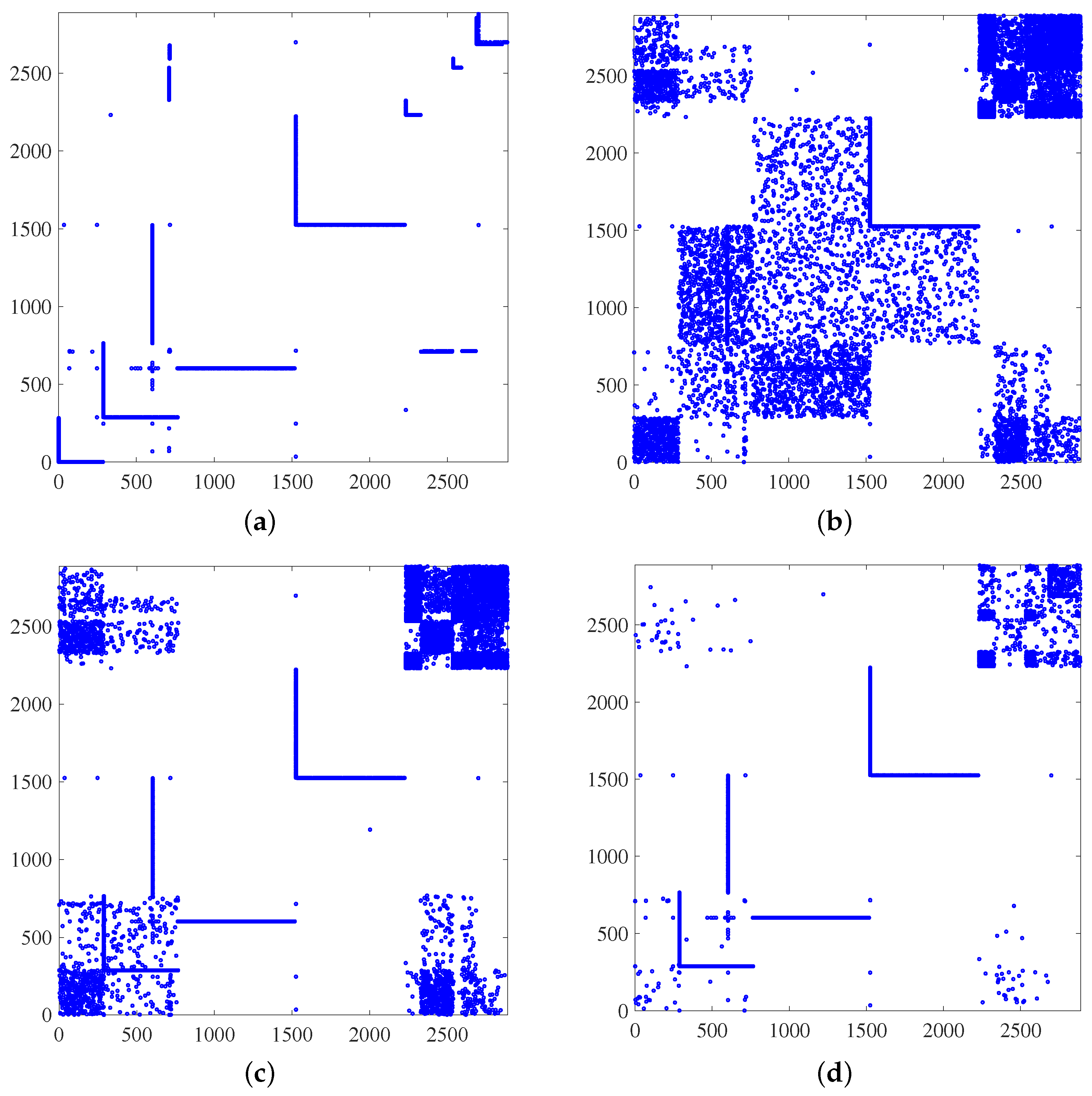
To evaluate the scalability of Algorithm 1, consider a directed network of $N=2888$ Facebook users, where the 2981 edges represent friendships among the users [50,51]. More precisely, an edge from node i to node j exists if user i is a friend of the user j. To make the graph amenable to our framework, we assume that the friendships are bilateral and ignore the directions. First, we notice that $\mathrm{rank}\left({\mathbf{W}}_{\mathcal{D}}\right)=2882$ (cf. Proposition 1). This means that knowing the GSO’s eigenvectors and $k=6$ suitably chosen edges as a priori information would lead to a singleton feasibility set. To test Algorithm 1 in recovering this reasonably large-scale graph, the performance is averaged over 10 experiments wherein we assume that we know the existence of $|\Omega |=5$ randomly sampled edges in each experiment. We then generate $T={10}^3$, ${10}^4$, ${10}^5$, or ${10}^6$ synthetic random signals ${\left\{{\mathbf{y}}_t\right\}}_{t=1}^T$ adhering to generative diffusion process in (2), where the entries of the inputs ${\left\{{\mathbf{x}}_t\right\}}_{t=1}^T$ are drawn independently from the standard Gaussian distribution to yield stationary observations. We obtain ${\widehat{\mathbf{C}}}_{\mathbf{y}}$ via a sample covariance estimate. For the aforementioned different values of T, the recovered $\widehat{\mathbf{S}}$ obtained after running Algorithm 1 results in the following F-measures.

Number of observations $\left(T\right)$	${10}^3$	${10}^4$	${10}^5$	${10}^6$
F-measure	$0.45$	$0.77$	$0.87$	$0.94$

As the number of observations increases, the estimate ${\widehat{\mathbf{C}}}_{\mathbf{y}}$ becomes more reliable which leads to a better performance in recovering the underlying GSO; recall that perfect support recovery corresponds to an F-measure of 1. This is visually apparent from Figure 1, where we depict the ground-truth Facebook network along with the estimated graphs for $T={10}^4$, ${10}^5$, and ${10}^6$. Moreover, the reported results corroborate the effectiveness of Algorithm 1 in recovering large-scale graphs. Off-the-shelf algorithms utilized to solve related topology inference problems in [6] are not effective for graphs with more than a few hundred nodes.

3.2. Zachary’s Karate Club: Online

Next, we consider the social network of Zachary’s karate club ([1], Ch. 1.2.2) represented by a graph $\mathcal{G}$ consisting of $N=34$ nodes or members of the club and 78 undirected edges symbolizing friendships among them. We seek to infer this graph from the observation of diffusion processes that are synthetically generated via graph filtering as in (2). The rank of ${\mathbf{W}}_{\mathcal{D}}$ (cf. Proposition 1) for this graph is 32. This implies that the knowledge of the perfect output covariance ${\mathbf{C}}_{\mathbf{y}}$ leaves the GSO $\mathbf{S}$ in a 2-dimensional subspace which can lead to singleton feasibility set by observing only two different edges. However, here we work with a noisy sample covariance ${\widehat{\mathbf{C}}}_{\mathbf{y}}$. We observe one of the 78 edges (chosen uniformly at random) and aim to infer the rest of the edges. At each time step, 10 synthetic signals $\left\{{\mathbf{y}}_p\right\}$ are generated through a diffusion process $\mathbf{H}$ where the entries of the inputs $\left\{{\mathbf{x}}_p\right\}$ are drawn independently from the standard Gaussian distribution. In the online case, upon sensing 10 signals at each time step, we first update the sample covariance ${\widehat{\mathbf{C}}}_{\mathbf{y},t}$ and then carry out $i_t=10$ PG iterations as Algorithm 2. To examine the tracking capability of the online estimator, after 5000 time steps, we remove $10\%$ of the existing edges and add the same number of edges elsewhere. This would affect the graph filter $\mathbf{H}$ accordingly.

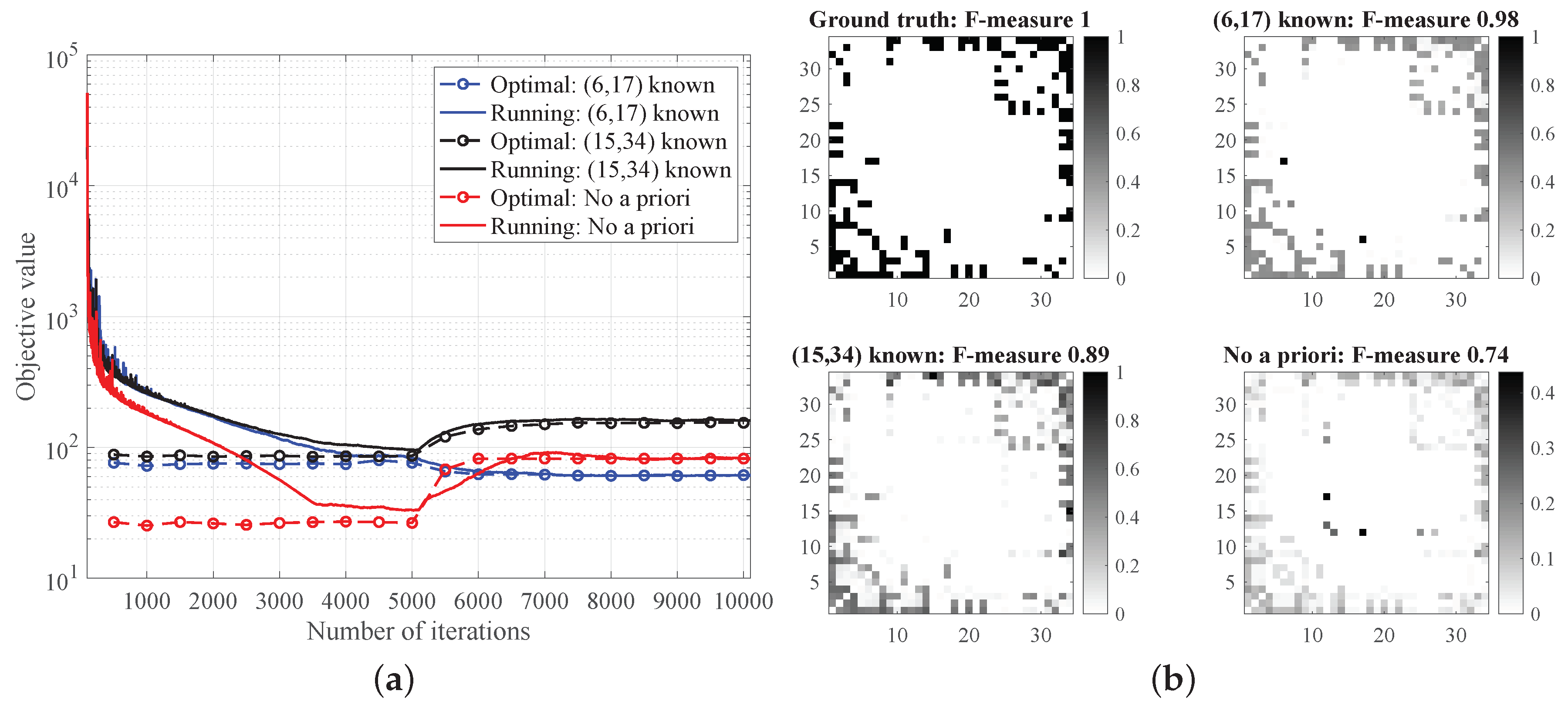
To corroborate the assumption in Theorem 1, it is worth mentioning that throughout the process we observed that ${\Psi }_{t,{\mathcal{D}}^c}$ was full column rank and thus the cost in (13) was strongly convex; see Proposition 2. Figure 2a depicts the running objective value $F_t\left({\mathbf{S}}_t\right)$ [cf. (13)] averaged over 10 experiments as a function of the time steps and the available a priori knowledge—two randomly chosen edges as well as the case where we have no a priori information on the edges ($\Omega =\varnothing$). For the latter case, we modify the feasible set $\mathcal{S}$ as suggested in Remark 2 as well as Algorithm 2 by implementing the proximal operator in (16). We also superimpose Figure 2a with the optimal objective value $F_t\left({\mathbf{S}}_t^{*}\right)$ at each time step. First, we notice that the objective value trajectory converges to a region above the optimal trajectory. We observe that after 5000 iterations, the performance deteriorates at first due to the sudden change of the network structure, but after observing enough new samples Algorithm 2 can adapt and track the batch estimator as well. This demonstrates the effectiveness of the developed online algorithm when it comes to adapting to network perturbations.

Finally, we study the quality of the graph ${\mathbf{S}}_t$ learned in an online fashion at iteration 5000 (just before the perturbation). Figure 2b depicts the heat maps of the ground-truth and inferred adjacency matrices for different a priori information. Although the procedure results in a slight gap between $F_t\left({\mathbf{S}}_t^{*}\right)$ and $F_t\left({\mathbf{S}}_t\right)$, it still reveals the underlying support of $\mathbf{A}$ with reasonable accuracy. Inspection of the F-measures in Figure 2b calculated on the thresholded adjacency matrices reveals that, as expected, having a priori information on the edges aids graph recovery performance.

4. Discussion

Here we include a brief but general discussion about the approach followed (and the assumptions made), its limitations as well as the impact this work can have to applications.

Our focus has been to develop efficient online algorithms for learning graphs from observations of stationary signals. We adopt a fairly general model where we require that second-order statistical dependencies of the observed signals to be explained by the unknown network structure. Stationarity and linear graph-filtering models (cf. (1)) can be accurate for real-world signals generated through a physical process akin to network diffusion. Examples include information cascades spreading over social networking platforms, vehicular mobility patterns, consensus dynamics, and progression of brain atrophy [4]. In our own prior work we have developed batch estimators of the form (5) to effectively recover the structural properties of proteins [6], to unveil urban mobility patterns, to cluster firms using a network learned from their historical stock prices [30], and to explore the relationship between functional and structural brain connectivities [52]. We believe the algorithms in this paper can have an impact on these and other related application domains, especially when network data is acquired in a streaming fashion. This direction certainly deserves further investigation. Relative to other useful approaches that postulate a more restricted family of generative graph filters (e.g., the parametric heat diffusion model in [25]), the more data-driven perspective advocated here can accommodate broader signal classes—possibly at the price of a larger sample complexity. Indeed, as our results show, one may require in the order of a million signals to accurately estimate a graph with $N=34$ vertices.

On the relevance of graph learning with partial connectivity information, consider link prediction that is a widely studied and canonical network topology inference problem. The goal is to infer whether or not unobserved pairs of vertices do or do not have an edge between them (i.e., inference of edge or non-edge status), using measurements that include a limited subset $\Omega$ of vertex pairs whose edge/no-nedge status is already observed; see e.g., ([1], Ch. 7.2) for a more formal definition of the link prediction problem. In this context, our rationale in this paper is to add some elements of link prediction to the earlier treatment of graph learning from observations of diffused, stationary signals [6,10]. We believe there is value in exploring how this extra prior information—when available—could be exploited to obtain simpler algorithmic updates and better recovery performance (see also Proposition 1 and the comparisons reported in Section 3.2).

There are various practical reasons as to why would only have access to observations of a subset of edges. If there is a temporal component to the graph learning problem, information about edges might be ‘missing’ only in the sense they are absent up to a certain point in time and then become present. In many time-invariant scenarios, the status of most edges might be unavailable due to issues of sampling (either because it is not affordable to measure all pairwise relationships, or just unfeasible due to the scale of the system or privacy constraints). For an exhaustive list of examples from information, biological, social and technological networks, the interested reader is referred to ([1], Ch. 7.2). In other cases, one could have a strong prior belief on the presence or absence of a few edges. It is thus only reasonable to include those as constraints to simplify the problem. For instance, in related work, we have looked at the inference of urban mobility graphs from Uber pick-up data in New York City [30]. With a very high degree of confidence, one expects there should be edges connecting the airports (JFK, Newark, LaGuardia) to a touristic epicenter such as Times Square, so it is prudent to add those to $\Omega$ and likely aid graph recovery performance. In any event, as explained in Remark 2 the partial connectivity assumption is not limiting. Most of the algorithms and theory developed here are valid when $\Omega =\varnothing$.

5. Conclusions

We studied the problem of identifying the topology of an undirected network from streaming observations of stationary signals diffused on the unknown graph. This is an important problem, because as a general principle network structural information can be used to understand, predict, and control the behavior of complex systems. The stationarity assumption implies that the observations’ covariance matrix and the GSO commute under mild requirements. This motivates formulating the topology inference task as an inverse problem, whereby one searches for a (e.g., sparse) GSO that is structurally admissible and approximately commutes with the observations’ empirical covariance matrix. For streaming data said covariance can be updated recursively, and we show online proximal gradient iterations can be brought to bear to efficiently track the time-varying solution of the inverse problem with quantifiable recovery guarantees. Ongoing work includes extensions of the online graph learning framework to observations of streaming signals that are smooth on the sought network.

References

- Kolaczyk, E.D. Statistical Analysis of Network Data: Methods and Models; Springer: New York, NY, USA, 2009. [Google Scholar]
- Slavakis, K.; Giannakis, G.B.; Mateos, G. Modeling and optimization for big data analytics: (Statistical) learning tools for our era of data deluge. IEEE Signal Process. Mag. 2014, 31, 18–31. [Google Scholar] [CrossRef]
- Ortega, A.; Frossard, P.; Kovačević, J.; Moura, J.M.F.; Vandergheynst, P. Graph signal processing: Overview, challenges and applications. Proc. IEEE 2018, 106, 808–828. [Google Scholar] [CrossRef] [Green Version]
- Mateos, G.; Segarra, S.; Marques, A.G.; Ribeiro, A. Connecting the dots: Identifying network structure via graph signal processing. IEEE Signal Process. Mag. 2019, 36, 16–43. [Google Scholar] [CrossRef] [Green Version]
- Dong, X.; Thanou, D.; Rabbat, M.; Frossard, P. Learning graphs from data: A signal representation perspective. IEEE Signal Process. Mag. 2019, 36, 44–63. [Google Scholar] [CrossRef] [Green Version]
- Segarra, S.; Marques, A.; Mateos, G.; Ribeiro, A. Network topology inference from spectral templates. IEEE Trans. Signal Inf. Process. Netw. 2017, 3, 467–483. [Google Scholar] [CrossRef]
- Marques, A.G.; Segarra, S.; Leus, G.; Ribeiro, A. Stationary graph processes and spectral estimation. IEEE Trans. Signal Process. 2017, 65, 5911–5926. [Google Scholar] [CrossRef]
- Perraudin, N.; Vandergheynst, P. Stationary signal processing on graphs. IEEE Trans. Signal Process. 2017, 65, 3462–3477. [Google Scholar] [CrossRef]
- Girault, B. Stationary graph signals using an isometric graph translation. In Proceedings of the 2015 23rd European Signal Processing Conference (EUSIPCO), Nice, France, 31 August–4 September 2015; pp. 1516–1520. [Google Scholar]
- Pasdeloup, B.; Gripon, V.; Mercier, G.; Pastor, D.; Rabbat, M.G. Characterization and inference of graph diffusion processes from observations of stationary signals. IEEE Trans. Signal Inf. Process. Netw. 2018, 4, 481–496. [Google Scholar] [CrossRef] [Green Version]
- Parikh, N.; Boyd, S. Proximal algorithms. Found. Trends Optim. 2014, 1, 123–231. [Google Scholar]
- Beck, A.; Teboulle, M. A fast iterative shrinkage-thresholding algorithm for linear inverse problems. SIAM J. Imag. Sci. 2009, 2, 183–202. [Google Scholar] [CrossRef] [Green Version]
- Shafipour, R.; Hashemi, A.; Mateos, G.; Vikalo, H. Online topology inference from streaming stationary graph signals. In Proceedings of the 2019 IEEE Data Science Workshop (DSW), Minneapolis, MN, USA, 2–5 June 2019; pp. 140–144. [Google Scholar]
- Shafipour, R.; Mateos, G. Online network topology inference with partial connectivity information. In Proceedings of the 2019 IEEE 8th International Workshop on Computational Advances in Multi-Sensor Adaptive Processing (CAMSAP), Le gosier, Guadeloupe, 15–18 December 2019; pp. 226–230. [Google Scholar]
- Ahmed, T.; Bajwa, W.U. Correlation-based ultra high-dimensional variable screening. In Proceedings of the 2017 IEEE 7th International Workshop on Computational Advances in Multi-Sensor Adaptive Processing (CAMSAP), Curacao, Netherlands Antilles, 10–13 December 2017; pp. 1–5. [Google Scholar]
- Madden, L.; Becker, S.; Dall’Anese, E. Online sparse subspace clustering. In Proceedings of the 2019 IEEE Data Science Workshop (DSW), Minneapolis, MN, USA, 2–5 June 2019; pp. 248–252. [Google Scholar]
- Dempster, A.P. Covariance selection. Biometrics 1972, 28, 157–175. [Google Scholar] [CrossRef]
- Friedman, J.; Hastie, T.; Tibshirani, R. Sparse inverse covariance estimation with the graphical lasso. Biostatistics 2008, 9, 432–441. [Google Scholar] [CrossRef] [PubMed] [Green Version]
- Lake, B.M.; Tenenbaum, J.B. Discovering structure by learning sparse graphs. In Proceedings of the 32nd Annual Meeting of the Cognitive Science Society (CogSci 2010), Portland, OR, USA, 11–14 August 2010; pp. 778–783. [Google Scholar]
- Egilmez, H.E.; Pavez, E.; Ortega, A. Graph learning from data under Laplacian and structural constraints. IEEE J. Sel. Top. Signal Process. 2017, 11, 825–841. [Google Scholar] [CrossRef]
- Meinshausen, N.; Buhlmann, P. High-dimensional graphs and variable selection with the lasso. Ann. Stat. 2006, 34, 1436–1462. [Google Scholar] [CrossRef] [Green Version]
- Dong, X.; Thanou, D.; Frossard, P.; Vandergheynst, P. Learning Laplacian matrix in smooth graph signal representations. IEEE Trans. Signal Process. 2016, 64, 6160–6173. [Google Scholar] [CrossRef] [Green Version]
- Mei, J.; Moura, J.M.F. Signal processing on graphs: Causal modeling of unstructured data. IEEE Trans. Signal Process. 2017, 65, 2077–2092. [Google Scholar] [CrossRef]
- Kalofolias, V. How to learn a graph from smooth signals. In Proceedings of the International Conference on Artificial Intelligence and Statistics (AISTATS), Cadiz, Spain, 9–11 May 2016; pp. 920–929. [Google Scholar]
- Thanou, D.; Dong, X.; Kressner, D.; Frossard, P. Learning heat diffusion graphs. IEEE Trans. Signal Inf. Process. Netw. 2017, 3, 484–499. [Google Scholar] [CrossRef] [Green Version]
- Kalofolias, V.; Perraudin, N. Large scale graph learning from smooth signals. In Proceedings of the 7th International Conference on Learning Representations (ICLR), New Orleans, LA, USA, 6–9 May 2019. [Google Scholar]
- Chepuri, S.P.; Liu, S.; Leus, G.; Hero, A.O. Learning sparse graphs under smoothness prior. In Proceedings of the 2017 IEEE International Conference on Acoustics, Speech and Signal Processing (ICASSP), New Orleans, LA, USA, 5–9 March 2017; pp. 6508–6512. [Google Scholar]
- Rabbat, M.G. Inferring sparse graphs from smooth signals with theoretical guarantees. In Proceedings of the 2017 IEEE International Conference on Acoustics, Speech and Signal Processing (ICASSP), New Orleans, LA, USA, 5–9 March 2017; pp. 6533–6537. [Google Scholar]
- Berger, P.; Hannak, G.; Matz, G. Efficient graph learning from noisy and incomplete data. IEEE Trans. Signal Inf. Process. Netw. 2020, 6, 105–119. [Google Scholar] [CrossRef]
- Shafipour, R.; Segarra, S.; Marques, A.G.; Mateos, G. Identifying the topology of undirected networks from diffused non-stationary graph signals. IEEE Open J. Signal Process. 2020. (submitted; see also arXiv:1801.03862 [eess.SP]). [Google Scholar]
- Shafipour, R.; Segarra, S.; Marques, A.G.; Mateos, G. Network topology inference from non-stationary graph signals. In Proceedings of the 2017 IEEE International Conference on Acoustics, Speech and Signal Processing (ICASSP), New Orleans, LA, USA, 5–9 March 2017. [Google Scholar]
- Cardoso, J.; Palomar, D. Learning undirected graphs in financial markets. arXiv 2020, arXiv:2005.09958v3. [Google Scholar]
- Kalofolias, V.; Loukas, A.; Thanou, D.; Frossard, P. Learning time varying graphs. In Proceedings of the 2017 IEEE International Conference on Acoustics, Speech and Signal Processing (ICASSP), New Orleans, LA, USA, 5–9 March 2017; pp. 2826–2830. [Google Scholar]
- Vlaski, S.; Maretić, H.P.; Nassif, R.; Frossard, P.; Sayed, A.H. Online graph learning from sequential data. In Proceedings of the 2018 IEEE Data Science Workshop (DSW), Lausanne, Switzerland, 4–6 June 2018; pp. 190–194. [Google Scholar]
- Shen, Y.; Baingana, B.; Giannakis, G.B. Tensor decompositions for identifying directed graph topologies and tracking dynamic networks. IEEE Trans. Signal Process. 2017, 65, 3675–3687. [Google Scholar] [CrossRef]
- Isufi, E.; Loukas, A.; Simonetto, A.; Leus, G. Autoregressive moving average graph filtering. IEEE Trans. Signal Process. 2017, 65, 274–288. [Google Scholar] [CrossRef] [Green Version]
- Baingana, B.; Mateos, G.; Giannakis, G.B. Proximal-gradient algorithms for tracking cascades over social networks. IEEE J. Sel. Top. Signal Process. 2014, 8, 563–575. [Google Scholar] [CrossRef]
- Giannakis, G.B.; Shen, Y.; Karanikolas, G.V. Topology identification and learning over graphs: Accounting for nonlinearities and dynamics. Proc. IEEE 2018, 106, 787–807. [Google Scholar] [CrossRef]
- Dall’Anese, E.; Simonetto, A.; Becker, S.; Madden, L. Optimization and learning with information streams: Time-varying algorithms and applications. IEEE Signal Process. Mag. 2020, 37, 71–83. [Google Scholar] [CrossRef]
- Di Lorenzo, P.; Banelli, P.; Barbarossa, S.; Sardellitti, S. Distributed adaptive learning of graph signals. IEEE Trans. Signal Process. 2017, 65, 4193–4208. [Google Scholar] [CrossRef] [Green Version]
- Di Lorenzo, P.; Banelli, P.; Isufi, E.; Barbarossa, S.; Leus, G. Adaptive graph signal processing: Algorithms and optimal sampling strategies. IEEE Trans. Signal Process. 2018, 66, 3584–3598. [Google Scholar] [CrossRef] [Green Version]
- Ioannidis, V.N.; Shen, Y.; Giannakis, G.B. Semi-blind inference of topologies and dynamical processes over dynamic graphs. IEEE Trans. Signal Process. 2019, 67, 2263–2274. [Google Scholar] [CrossRef] [Green Version]
- Daubechies, I.; Defrise, M.; Mol, C.D. An iterative thresholding algorithm for linear inverse problems with a sparsity constraint. Commun. Pure Appl. Math. 2004, 57, 1413–1457. [Google Scholar] [CrossRef] [Green Version]
- Wright, S.J.; Nowak, R.D.; Figueiredo, M.A.T. Sparse reconstruction by separable approximation. IEEE Trans. Signal Process. 2009, 57, 2479–2493. [Google Scholar] [CrossRef] [Green Version]
- Beck, A. First-Order Methods in Optimization; Society for Industrial and Applied Mathematics: Philadelphia, PA, USA, 2018. [Google Scholar]
- Bauschke, H.H.; Combettes, P.L. Convex Analysis and Monotone Operator Theory in Hilbert Spaces; Springer: Berlin, Germany, 2011; Volume 408. [Google Scholar]
- Nesterov, Y. Smooth minimization of nonsmooth functions. Math. Prog. 2005, 103, 127–152. [Google Scholar] [CrossRef]
- Chen, Y.; Ye, X. Projection onto a simplex. arXiv 2011, arXiv:1101.6081. [Google Scholar]
- Solo, V.; Kong, X. Adaptive Signal Processing Algorithms: Stability and Performance; Prentice Hall: Upper Saddle River, NJ, USA, 1995. [Google Scholar]
- Kunegis, J. KONECT—The Koblenz Network Collection. In Proceedings of the 22nd International Conference on World Wide Web (WWW’13 Companion), Rio de Janeiro, Brazil, 13–17 May 2013; pp. 1343–1350. [Google Scholar]
- Leskovec, J.; Mcauley, J. Learning to discover social circles in ego networks. In Proceedings of the Advances in Neural Information Processing Systems (NIPS), Lake Tahoe, Nevada, 3–6 December 2012; pp. 539–547. [Google Scholar]
- Li, Y.; Mateos, G. Identifying Structural Brain Networks from Functional Connectivity: A Network Deconvolution Approach. In Proceedings of the IEEE International Conference on Acoustics, Speech and Signal Processing (ICASSP), Brighton, UK, 12–17 May 2019; pp. 1135–1139. [Google Scholar]
Figure 1.
Recovery of Facebook friendship graph with nodes. Adjacency matrix of (a) ground-truth network; and estimates for (b) ; (c) ; and (d) . It is apparent how recovery performance markedly improves as the sample size increases; see also the accompanying table with the corresponding F-measure values.
Figure 2.
Recovery of Zachary’s karate club graph with nodes. (a) Evolution of the objective values for the online and batch estimators in inferring a karate club. (b) Ground-truth adjacency matrix and corresponding estimates after 5000 time steps, for different prior connectivity information settings. Knowledge of at least one edge in the graph can markedly improve support recovery performance as indicated by the obtained F-measure values.
© 2020 by the authors. Licensee MDPI, Basel, Switzerland. This article is an open access article distributed under the terms and conditions of the Creative Commons Attribution (CC BY) license (http://creativecommons.org/licenses/by/4.0/).
Share and Cite
MDPI and ACS Style
Shafipour, R.; Mateos, G. Online Topology Inference from Streaming Stationary Graph Signals with Partial Connectivity Information. Algorithms 2020, 13, 228. https://0-doi-org.brum.beds.ac.uk/10.3390/a13090228
AMA Style
Shafipour R, Mateos G. Online Topology Inference from Streaming Stationary Graph Signals with Partial Connectivity Information. Algorithms. 2020; 13(9):228. https://0-doi-org.brum.beds.ac.uk/10.3390/a13090228
Chicago/Turabian StyleShafipour, Rasoul, and Gonzalo Mateos. 2020. "Online Topology Inference from Streaming Stationary Graph Signals with Partial Connectivity Information" Algorithms 13, no. 9: 228. https://0-doi-org.brum.beds.ac.uk/10.3390/a13090228
Note that from the first issue of 2016, this journal uses article numbers instead of page numbers. See further details here.