Efficient Approaches to the Mixture Distance Problem


1
Department of Computer Science and Information Engineering, National Chi Nan University, Puli, Nantou 54561, Taiwan
2
Department of Computer Science and Information Engineering, National Taiwan University, Taipei 10617, Taiwan
3
Department of Mathematics and Statistics, Idaho State University, Pocatello, ID 83209, USA
*
Author to whom correspondence should be addressed.
Algorithms 2020, 13(12), 314; https://0-doi-org.brum.beds.ac.uk/10.3390/a13120314
Submission received: 31 August 2020
/
Revised: 19 November 2020
/
Accepted: 23 November 2020
/
Published: 28 November 2020
(This article belongs to the Special Issue Graph Algorithms and Applications)
Abstract
:The ancestral mixture model, an important model building a hierarchical tree from high dimensional binary sequences, was proposed by Chen and Lindsay in 2006. As a phylogenetic tree (or evolutionary tree), a mixture tree created from ancestral mixture models, involves the inferred evolutionary relationships among various biological species. Moreover, it contains the information of time when the species mutates. The tree comparison metric, an essential issue in bioinformatics, is used to measure the similarity between trees. To our knowledge, however, the approach to the comparison between two mixture trees is still unknown. In this paper, we propose a new metric named the mixture distance metric, to measure the similarity of two mixture trees. It uniquely considers the factor of evolutionary times between trees. If we convert the mixture tree that contains the information of mutation time of each internal node into a weighted tree, the mixture distance metric is very close to the weighted path difference distance metric. Since the converted mixture tree forms a special weighted tree, we were able to design a more efficient algorithm to calculate this new metric. Therefore, we developed two algorithms to compute the mixture distance between two mixture trees. One requires and the other requires computational time with preprocessing time, where n denotes the number of leaves in the two mixture trees, and and denote the heights of these two trees.
1. Introduction
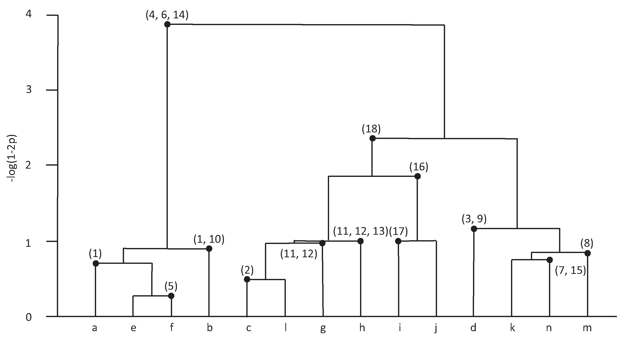
Phylogeny reconstruction involves reconstructing the evolutionary relationship from biological sequences among species. Nowadays it has become a critical issue in molecular biology and bioinformatics. Several existing methods, such as neighbor-joining methods [1] and maximum likelihood methods [2], have been proposed to reconstruct a phylogenetic tree. A novel and natural method, ancestral mixture models [3], was developed by Chen and Lindsay to deal with such a problem. The mixture tree, a hierarchical tree created from the ancestral mixture model, induces a sieve parameter to represent the evolutionary time. Chen, Rosenberg and Lindsay (2011) then developed MixtureTree algorithm [4], a linux based program written in C++, which employed the ancestral mixture models to reconstruct mixture tree from DNA sequences. With the information provided by the mixture tree, one can identify when and how a mutation event of species occurs. An example of the mixture tree created by MixtureTree algorithm [3] is shown in Figure 1. The data from Griffiths and Tavare (1994) [5] are a subset of the mitochondrial DNA sequences which first appeared in Ward et al. (1991) [6]. To study the mitochondrial diversity within the Nuu-Chuah-Nulth, an Amerindian tribe from Vancouver Island, Ward et al. (1991) [6] sequenced 360 nucleotide segments of the mitochondrial control region for 63 individuals from the Nuu-Chuah-Nulth. Griffiths’ and Tavares’ subsample consisted of 55 of the 63 distinct sequences and 18 segregating sites, including 13 pyrimidines (C, T ) and five purines (A, G). Each linage represents a distinct sequence—that is, there are lineages a through n. The time scale on the tree can be represented by , where p is a parameter, the mutation rate. The number on the tree represents the site of the lineage whereat the mutation occurs. For example, when , lineages e and f merge because mutation occurs at site 5 of lineage f.
Distinct methods may produce distinct trees, even though the methods adopt an identical dataset [7]. To uncover a well-represented tree involved in evolutionary relationship among species it is quite important to estimate how similar (or different) trees are. The tree distance between two trees is a general measurement for the similarity of the trees.
The tree distance problem is a traditional issue in mathematics. Several metrics have been proposed to measure the similarity between two trees, such as the partition metric (also called the Robison–Foulds metric or RF distance for short) [8], the quartet metric [9], the nearest neighbour interchange metric [10] and the nodal distance metric [11]. Those metrics all compare two trees by considering the tree structure only, and do not mention any parameter in the tree. Thus, those metrics are not suitable for computing the similarity between two mixture trees. Therefore, we propose a novel metric named the mixture distance metric to measure the similarity of two mixture trees in this paper. Among the above metrics, the metric from the nodal distance algorithm is similar to our proposed metric. In 2003, John Bluis and Dong-Guk Shin [11] presented the nodal distance algorithm which is used to measure the distances from leaves to all other leaves in a tree. The metric is defined as follows: Distance , where denotes the distance of leaf x to leaf y in the tree . The nodal distance algorithm was developed for this metric. Anyway, using this metric to measure the distance between two mixture trees is not conformable.
For the metric of the mixture distance, the time parameter indicating when a mutation event of species occurs plays an important role in the tree similarity, which is, however, not considered by those previous metrics. If the weight of an edge in a mixture tree is defined as the difference in time parameters between its two endpoints, a mixture tree can be regarded as a weighted tree. We can design metrics to calculate the distance between two weighted trees. Some literature discusses the distance problem between two weighted trees. For example, take the weighted RF metric [12], geodesic distance [13] and the path difference metric [14]. However, the weight on each edge is considered to be the number of base changes between the sequences of the species represented by its incident vertices in these documents. Since the weights of each edge in those weighted trees may be different, the algorithm must spend more time to calculate those distances between those two weighted trees. For example, although there is an linear time algorithm to compute RF distance [15], and a randomized algorithm has been shown to approximate the RF distance with a bounded error in sublinear time [16], the complexity of the weighted RF distance still needs . Some papers have studied algorithms for calculating the geodesic trees distances [17,18,19]. The best one already known is [19]. Due to the characteristics of the time parameter of a mixture tree, any two edges connecting two leaves to the same parent will have the same “weight” in a mixture tree. This helped us to design a better metric and algorithm. We further developed two algorithms to compute the mixture distance between two mixture trees. One requires and the other requires computational time with preprocessing time, where n denotes the number of leaves in these two mixture trees, and and denote the heights of these two trees. If we use the nodal distance algorithm with the mixture distance metric, the time complexity will be for binary unrooted trees. Comparisons with some previous methods show our method performs better.
2. Mixture Distance Metric
A tree is a connected and acyclic graph with a node set and an edge set . T is a rooted tree if exactly one node of T has been designated the root. A node is a leaf if it has no child; otherwise, v is an internal node. A node is called in level i, denoted by , which means the number of edges on the path between the root and v is i. Let denote a subset of node set , where each member is a leaf in T and . Let denote the height of tree T, which is max. T is a full binary tree if each node of T either has two children or it is a leaf. A complete binary tree is a full binary tree in which every level, except possibly the last, is completely filled, and all nodes are as far left as possible. Let , .
For a mixture tree T, each leaf is associated with a species, and every internal node v is associated with a mutation time that represents the time when a mutation event occurs on the species node. In fact, the mutation time of an internal node in a mixture tree can be regarded as the distance between the node and any leaf of its descendants. Any two mixture tress and are comparable if . Throughout this paper, a tree refers to a rooted full binary tree and each internal node of the tree is associated with its mutation time, if not mentioned particularly.
Given any two nodes , the least common ancestor or lowest common ancestor (abbreviated LCA) of u and v is an ancestor of both u and v with the smallest mutation time. (It is also called the most recent common ancestor (abbreviated MRCA), or the last common ancestor (abbreviated LCA) in biology and genealogy.) Let denote the mutation time of the LCA w of two leaves u and v in T. The mixture distance metric, a metric for the mixture tree, is formally defined as follows.
The mixture distance between two comparable mixture trees and , denoted by , is defined as the sum of difference of the mutation times with respect to the LCAs of any two leaves in and . That is, =
The significance of the mixture distance metric is to measure the similarity between two mixture trees, considering the mutation times (molecular clock) and mutation sites simultaneously. The study sought to develop two algorithms for efficiently computing the mixture distance between two comparable mixture trees. Before we go into the algorithms, three properties of the mixture distance matric are demonstrated. Felsenstein [20] derived three mathematical properties—reflexivity, symmetry and triangle inequality—required for a well-defined metric. We show that the mixture distance is well-defined in Theorem 1.
Theorem 1.
The mixture distance satisfies:
- 1.
- Reflexivity: for any two comparable mixture trees and , if and only if and are identical.
- 2.
- Symmetry: for any two comparable mixture trees and , .
- 3.
- Triangle inequality: for any three comparable mixture trees , and , .
Proof.
1. Due to , for any two nodes , we have . Therefore, can be concluded. On the other hand, if for any two comparable mixture trees and . We have for any by the definition. Then we can prove by induction on the height of (or ).
2. For any two nodes , . Thus, .
3. The triangle inequality is always satisfied for any three nonnegative numbers ; that is, . Therefore, holds. Further, we have
Consequently, can be concluded. □
3. An -Time Algorithm
Let and denote two comparable mixture trees of n leaves for each tree. Note that the mixture distance of and can be solved in -time: As when given two comparable mixture trees and each with n leaves, there are pairs of leaves separately in and . In fact, the LCA of any pair of leaves can be found by adopting the -time algorithm with -time preprocessing [21].
In the following, another -time algorithm, named Algorithm MixtureDistance, is proposed to compute the mixture distance between and , which will help us to realize the next -time algorithm, the main result.
3.1. Algorithm MixtureDistance
Algorithm MixtureDistance, as shown on Algorithm 1, proceeds the nodes of by breadth-first search. For each internal node v in , we find out the leaves of such that v is exactly the LCA of each pair of leaves, and then compute the LCA u of the leaves in which are mapped into the found leaves of . Finally, the difference of the mutation times between u and v is calculated. For convenience, we define for any two ordered pairs and in this algorithm, where and d are any four integers.
The algorithm adopts a 2-coloring method [22] on the leaves in and for easy implementation. For each iteration associated with an internal node v of in line 4, the leaves of the left and right subtrees rooted by v are colored by red and green, respectively. The mapped leaves in have the same coloring as one in . The mixture distance between each internal node u in and v is calculated according the coloring scheme in (in lines 16–17), and the coloring information of u would be derived for the computation of its parent node (in line 18).
The coloring information of u, denoted by , indicates the coloring information of the subtree in rooted by u. includes two numbers of u’s descendant leaves colored by red () and green (), respectively. is derived by the coloring information of its two children. That is, and , where and separately denote the left and right children of u in .
| Algorithm 1: MixtureDistance. |
| Input: Two comparable mixture trees and , with mutation times (, respectively) for every internal node v of (u of , respectively). |
| Output: The mixture distance between and . |
| . |
| Traverse by the breadth-first search from its root and keep a list of the internal nodes in order. |
| Traverse by the breadth-first search from its root and keep a list of the internal nodes in reverse order. |
| for each node do |
| 5 In , color red the leaves of the left subtree rooted by v and green the leaves of the right subtree rooted by v. |
| 6 for each node do // Initialize the coloring information of u’s children |
| 7 for each child w of u in do |
| 8 if w is a leaf then |
| 9 if w is colored by red in then |
| 10 . |
| 11 else if w is colored by green in then |
| 12 . |
| 13 else |
| 14 . |
| 15 Let and be the left and right children of u in , respectively. // Calculate the difference of the mutation times of u and v and sum them up for computing mixture distance |
| 16 . |
| 17 . // Calculate the coloring information of u |
| 18 . |
In line 16, is achieved by the special product of the color vectors of u’s two children, , which means the number of times that u is an of a red leaf and a green leaf. We multiply the difference of their mutation times by in line 17, for computing the mixture distance between each internal node u in and v. At the end of Algorithm MixtureDistance, indicates the mixture distance of and .
Since the numbers of internal nodes in and ( and ) are both equal to , two for-loops will take time, and the innermost for-loop always takes 2 (a constant) time units. Therefore, Algorithm MixtureDistance requires computational time.
3.2. Modified Algorithm
After introducing Algorithm MixtureDistance, we can give a computational time algorithm for computing the mixture distance between two mixture trees in the following part. In Algorithm MixtureDistance, when the leaves of the subtree rooted by an internal node v in are colored, other leaves in have no color, as do the mapped leaves in . That is, for . However, Algorithm MixtureDistance still processes the ancestors of such leaves in . In the following, we propose an algorithm for disregarding the nodes without meaningful coloring information, and reduce the time complexity from to .
The algorithm contains three main stages, as follows:
- Rank the leaves in and .
- Construct a minimal subtree of involved in colored leaves with respect to node v, for each internal node v in .
- Compute the mixture distance between v and each internal node in .
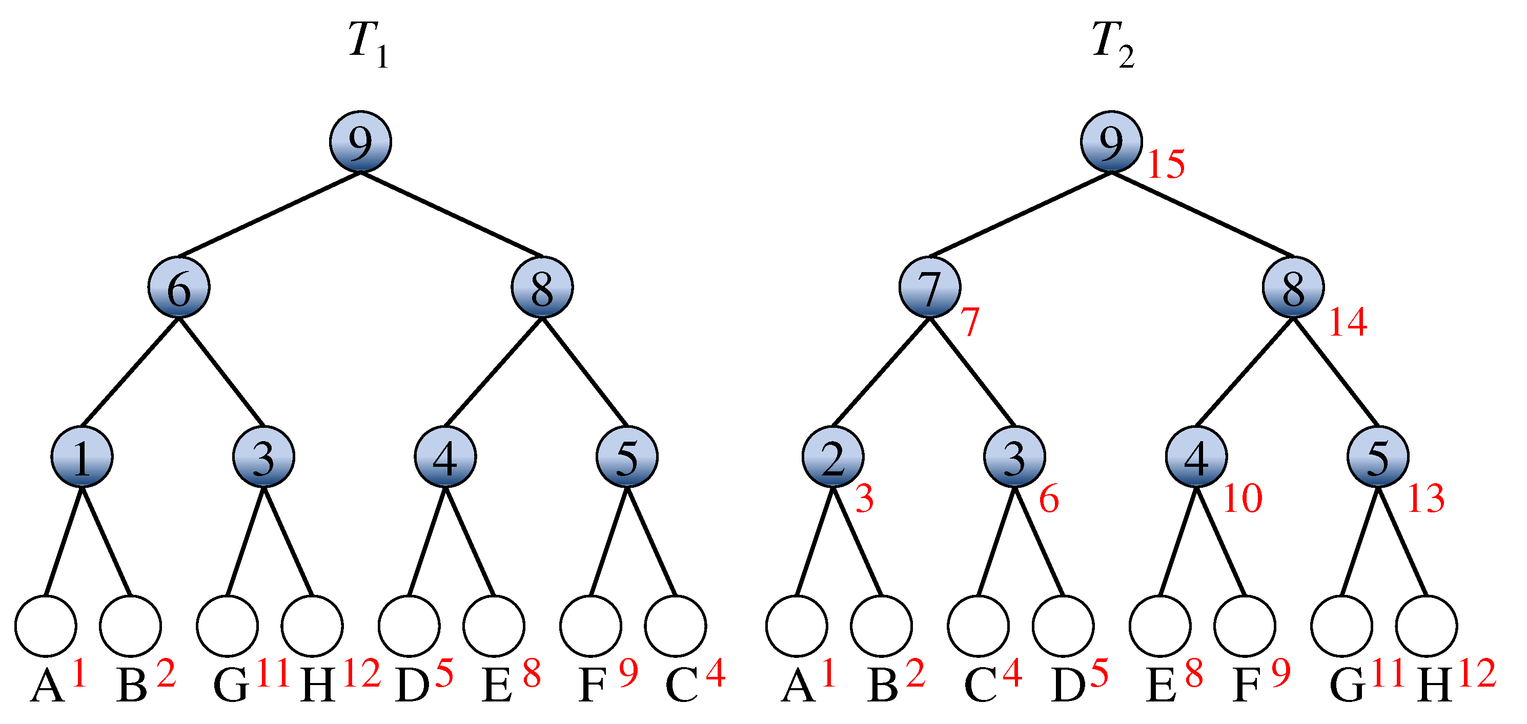
In stage 1, the nodes of are ranked in postorder, and the leaves of are assigned by the same rank of the mapped leaves in . In Figure 2, red numbers nearby leaves in two given comparable mixture trees and indicate the ranking achieved by stage 1 of the algorithm. Note that the number within the nodes means the mutation time of the associated node v for or 2.
The algorithm proceeds to stage 2 for each internal node v of in the reverse order of breadth-first search. When v in is processed, stage 2 seeks to construct a minimal subtree of involved in colored leaves with respect to node v. For node v, a nondecreasing list of the leaves of the subtree rooted by v, denoted by , is obtained from the leaf lists of its two children, where the leaves in the list are sorted by their ranks. Suppose that there are k ordered nodes in , that is, . With the list , the subtree can be constructed as follows.
Let denote the LCA of leaves and in , for any . The subtree is initialized by , and . For node , ,
Moreover, if the mutation time (the number written in the node circle) of , denoted by , is larger than the mutation time of , denoted by , the edge is inserted into and reset as the new . Otherwise, if is smaller than the mutation time of , denoted by , the edge is removed from and the edges and are inserted into . Otherwise, let x = and repeat do until , where is the node y such that . Then the edge is removed from and the edges and are inserted into .
Example 1.
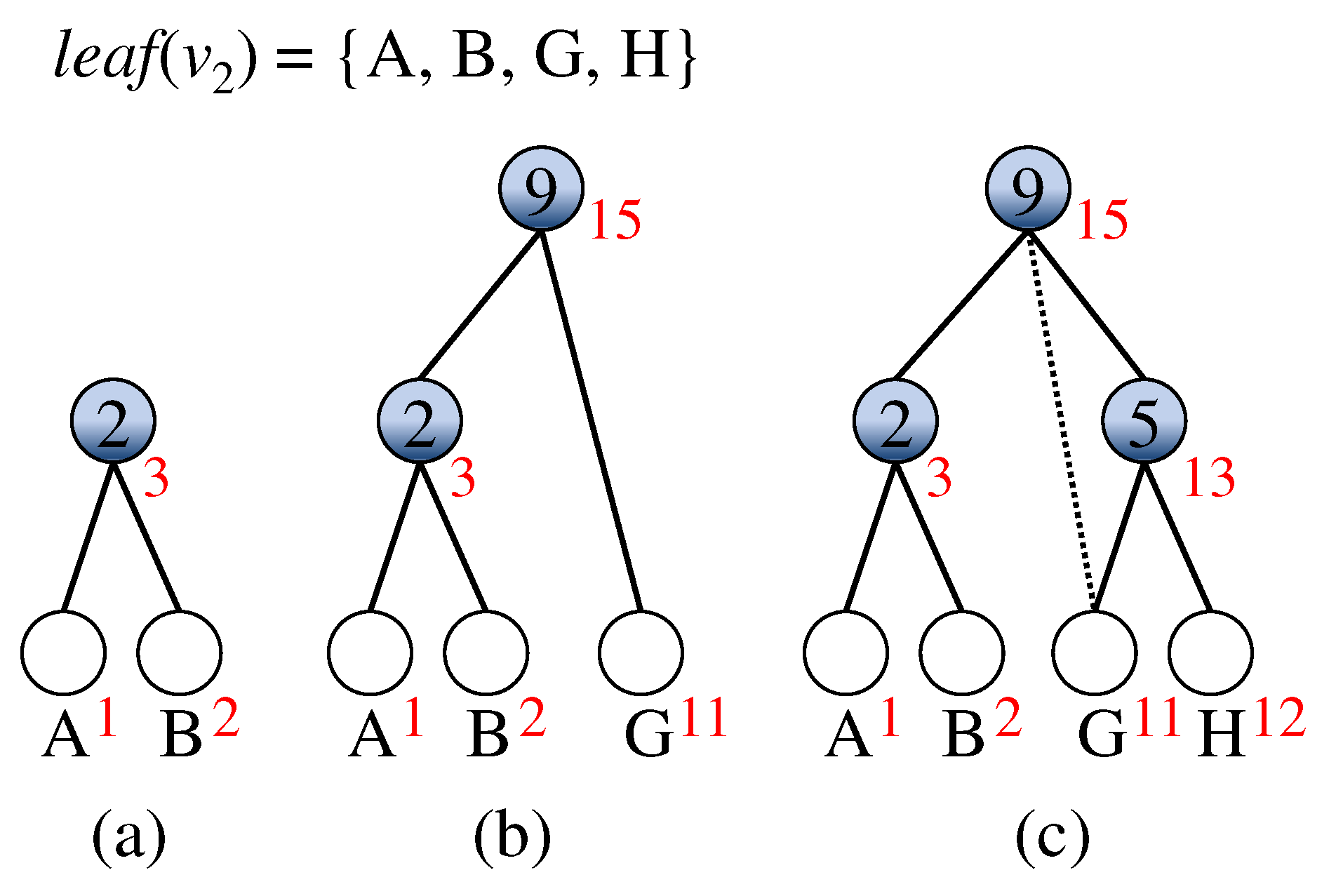
An example of constructing the subtree with respect to is illustrated in Figure 3. Initially, the node set is and the edge set includes the incident edges of the three nodes in . As node A is processed, two nodes and G are inserted into , and two edges and are inserted into . Later, when node B is processed, two nodes and H are inserted into and two edges and are inserted into . Meanwhile, the edge is removed from and the edge is inserted into , because the mutation time of is larger than the time of the .
After the subtree with respect to currently processed node v is constructed, stage 3 of the algorithm performs lines 5–18 of Algorithm MixtureDistance to compute the “partial” mixture distance between and the subtree rooted by v (only computes the distances of some nodes pairs, for which LCA is equal to v). At the end of the algorithm, indicates the mixture distance between and .
Theorem 2.
The improved algorithm takes computational time and preprocessing time, where n denotes the number of leaves of the mixture trees and for .
Proof.
The algorithm contains three main stages. The first stage ranks the leaves in and , which takes time.
In the second stage, a minimal subtree of involved in colored leaves with respect to each node v in is constructed. For each node v, a leaf list is obtained from the leaf lists of its two children, which is achieved in time by using the two-way merging algorithm [23] performed on the leaf list of v’s children, where t is the size of . The -time algorithm with -time processing [21] is employed to compute the LCA of any pair of nodes in . Constructing takes time, where is the height of due to the “repeat” step. The last stage computes the mixture distance between v and each internal node in by performing lines 5–18 of Algorithm MixtureDistance, which takes time. Stages 2 and 3 take iterations in total. However, each iteration deals with different t nodes. Note that for all internal nodes which are in the same level of , the sum of t (for each node) is n. Therefore, stages 2 and 3 totally take time, where is the height of (note that ). Hence, the algorithm requires computational time with preprocessing time. □
4. Conclusions
In this paper, we provide a novel metric named the mixture distance metric to measure the similarity between two mixture trees. It uniquely considers the estimated evolutionary time in the trees. Two algorithms were developed to compute the mixture distance between mixture trees. One requires computational time and the other requires computational time with preprocessing time, respectively. Note that when and are complete binary trees, and will be and the time complexity of our algorithm will be .
Now, we compare our metric with some previous methods which measure phylogenetic differences in consideration of the branch length, when we consider a mixture tree as a weighted tree (recall that the weight of an edge in a mixture tree is defined as the difference of time parameters between its two endpoints). For the geodesic tree distance, the implementation is quite complex and requires heavy computation [19], although a heuristic fast version exists [18]. The definition of the weighted path difference distance [14] is almost the same as the mixture distance. Actually, the weighted path difference distance between two mixture trees and is equal to . However, it requires computational time. The mixture distance seems to be similar to the weighted RF distance [12], but the calculation performance will vary when we consider the distance between two different extents of similar mixture trees. We give an example as follows.
Example 2.
Four mixture trees with the same lineages A, B and C are illustrated in Figure 4; the time parameters are listed in the vertices, and the associated edge weights are labeled beside each edge. All pairs of these four trees have been compared using the methods outlined in [12] and this paper. The tables of the weighted RF (wRF) and mixture distances () are given in Table 1 and Table 2, respectively. From these two tables, one can find something interesting. (1) seems maintain the order relationship in wRF: When wRF thinks that two trees are similar, then also gets a smaller value between these two trees: wRF wRF wRF wRF and . (2) When wRF thinks that the distances between two pairs of trees are the same, then also thinks they are in the same: wRF wRF, wRF wRF and , . However, there are still differences between these two metrics in the details: (3) When wRF thinks two distances between two pairs of trees are very different, sometimes may not think that: wRF wRF, wRF wRF, but .
Therefore, it can be said that the performance of the mixture distance in calculating the similarity of two weighted trees is as good as the performance of the weighted RF distance, while the time complexity of the mixture distance is better. In addition, we compared our approaches with the methods performed with the nodal distance metric [11], geodesic tree distance [19], weighted path difference metric [14] and weighted RF distance [12], and the results are shown in Table 3. Our proposed approaches performed better than all of the previous methods when discussing the distance between two mixture trees.
Author Contributions
Investigation, Y.-C.C. and C.-H.L.; methodology, J.S.-T.J. and S.-C.C. All authors have read and agreed to the published version of the manuscript.
Funding
The first author was supported in part by the Ministry of Science and Technology of the Republic of China under Contract No. MOST100-2221-E-260-024- and MOST109-2115-M-260-001.
Conflicts of Interest
The authors declare no conflict of interest.
References
- Saitou, N.; Nei, M. The neighbor-joining method: A new method for reconstructing phylogenetic trees. Mol. Biol. Evol. 1987, 4, 406–425. [Google Scholar] [PubMed]
- Lesperance, M.L.; Kalbfleisch, J.D. An algorithm for computing the nonparametric MLE of a mixing distribution. J. Am. Stat. Assoc. 1992, 87, 120–126. [Google Scholar] [CrossRef]
- Chen, S.C.; Lindsay, B.G. Building mixture trees from binary sequence data. Biometrika 2006, 93, 843–860. [Google Scholar] [CrossRef] [Green Version]
- Chen, S.C.; Rosenberg, M.; Lindsay, B.G. MixtureTree: A program for constructing phylogeny. BMC Bioinform. 2011, 12, 111–114. [Google Scholar] [CrossRef] [PubMed] [Green Version]
- Griffiths, R.C.; Tavare, S. Ancestral inference in population genetics. Statist. Sci. 1994, 9, 307–319. [Google Scholar] [CrossRef]
- Ward, R.H.; Frazier, B.L.; Dew-Jager, K.; Paabo, S. Extensive mitochondrial diversity within a single amerindian tribe. Proc. Nat. Acad. Sci. USA 1991, 88, 6720–6724. [Google Scholar] [CrossRef] [PubMed] [Green Version]
- Steel, M.A. The maximum likelihood point for a phylogenetic tree is not unique. Syst. Biol. 1994, 43, 560–564. [Google Scholar] [CrossRef]
- Robinson, D.F.; Foulds, L.R. Comparison of phylogenetic trees. Biosciences 1981, 53, 131–147. [Google Scholar] [CrossRef]
- Estabrook, G.F.; McMorris, F.R.; Meacham, C.A. Comparison of undirected phylogenetic trees based on subtrees of four evolutionary units. Syst. Zool. 1985, 34, 193–200. [Google Scholar] [CrossRef]
- Dasgupta, B.; He, X.; Jiang, T.; Li, M.; Tromp, J.; Zhang, L. On computing the nearest neighbor interchange distance. In Proceedings of the Discrete Mathematical Problems with Medical Applications: DIMACS Workshop on Discrete Problems with Medical Applications, Piscataway, NJ, USA, 8–10 December 1999; American Mathematical Society: Washington, DC, USA, 2000; Volume 55, pp. 125–143. [Google Scholar]
- Bluis, J.; Shin, D. Nodal distance algorithm: Calculating a phylogenetic tree comparison metric. In Proceedings of the Third IEEE Symposium on BioInformatics and BioEngineering, Bethesda, MD, USA, 12 March 2003; pp. 87–94. [Google Scholar]
- Robinson, D.F.; Foulds, L.R. Comparison of weighted labelled trees. In Combinatorial Mathematics VI; Springer: Berlin/Heidelberg, Germany, 1979; pp. 119–126. [Google Scholar]
- Billera, L.J.; Holmes, S.P.; Vogtmann, K. Geometry of the space of phylogenetic trees. Adv. Appl. Math. 2001, 27, 733–767. [Google Scholar] [CrossRef] [Green Version]
- Steel, M.A.; Penny, D. Distributions of tree comparison metrics—Some new results. Syst. Biol. 1993, 42, 126–141. [Google Scholar]
- Day, W.H. Optimal algorithms for comparing trees with labeled leaves. J. Classif. 1985, 2, 7–28. [Google Scholar] [CrossRef]
- Pattengale, N.D.; Gottlieb, E.J.; Moret, B.M. Efficiently computing the Robinson-Foulds metric. J. Comput. Biol. 2007, 14, 724–735. [Google Scholar] [CrossRef] [PubMed]
- Battagliero, S.; Puglia, G.; Vicario, S.; Rubino, F.; Scioscia, G.; Leo, P. An efficient algorithm for approximating geodesic distances in tree space. IEEE/ACM Trans. Comput. Biol. Bioinform. 2010, 8, 1196–1207. [Google Scholar] [CrossRef] [PubMed]
- Amenta, N.; Godwin, M.; Postarnakevich, N.; John, K.S. Approximating geodesic tree distance. Inf. Process. Lett. 2007, 103, 61–65. [Google Scholar] [CrossRef]
- Owen, M.; Provan, J.S. A fast algorithm for computing geodesic distances in tree space. IEEE/ACM Trans. Comput. Biol. Bioinform. 2010, 8, 2–13. [Google Scholar] [CrossRef] [PubMed] [Green Version]
- Felsenstein, J. Inferring Phylogenies; Sinauer Associates: Sunderland, MA, USA, 2004. [Google Scholar]
- Bender, M.A.; Farach-Colton, M. The LCA problem revisited. Lat. Am. Theor. Inform. 2000, 1776, 88–94. [Google Scholar]
- Brodal, G.S.; Fagerberg, R.; Pedersen, C.N.S. Computing the quartet distance between evolutionary trees in time O(nlogn). Algorithmica 2003, 38, 377–395. [Google Scholar] [CrossRef]
- Lee, R.C.T.; Chang, R.C.; Tseng, S.S.; Tsai, Y.T. Introduction to the Design and Analysis of Algorithms; McGraw-Hill Education: Berkshire, UK, 2005. [Google Scholar]
Figure 1.
An example of the mixture tree [3].
Figure 1.
An example of the mixture tree [3].

Figure 2.
An example of ranking leaves of and .

Figure 3.
An example of constructing the subtree with respect to in Figure 2. (a) The initialization of . (b) The intermediate of as node A is processed. (c) The complete subtree as node B is processed. As the mutation time of (B, G) is larger than the time of (G, H), the dotted line incident to G is removed and the other incident edge of G is inserted.

Figure 4.
Four weighted trees with the same lineages A, B and C.


Table 1.
The weighted RF distances wRF among , , and .
| wRF | ||||
|---|---|---|---|---|
| 3 | 8 | 7 | ||
| 7 | 4 | |||
| 3 |
Table 2.
The mixture distances among , , and .
| 1 | 4 | 3 | ||
| 3 | 2 | |||
| 1 |
Table 3.
Comparison of metrics for binary trees.
| Metric | Consideration | Time Complexity | |
|---|---|---|---|
| Full Binary Trees | Complete Binary Trees | ||
| Mixture distance | Structure and mutation time | ||
| Nodal distance | Structure | ||
| Geodesic tree distance | Structure and mutation number | ||
| Weighted path difference distance | Structure and mutation number | ||
| Weighted RF distance | Structure and mutation number | ||
Publisher’s Note: MDPI stays neutral with regard to jurisdictional claims in published maps and institutional affiliations. |
© 2020 by the authors. Licensee MDPI, Basel, Switzerland. This article is an open access article distributed under the terms and conditions of the Creative Commons Attribution (CC BY) license (http://creativecommons.org/licenses/by/4.0/).
Share and Cite
MDPI and ACS Style
Juan, J.S.-T.; Chen, Y.-C.; Lin, C.-H.; Chen, S.-C. Efficient Approaches to the Mixture Distance Problem. Algorithms 2020, 13, 314. https://0-doi-org.brum.beds.ac.uk/10.3390/a13120314
AMA Style
Juan JS-T, Chen Y-C, Lin C-H, Chen S-C. Efficient Approaches to the Mixture Distance Problem. Algorithms. 2020; 13(12):314. https://0-doi-org.brum.beds.ac.uk/10.3390/a13120314
Chicago/Turabian StyleJuan, Justie Su-Tzu, Yi-Ching Chen, Chen-Hui Lin, and Shu-Chuan Chen. 2020. "Efficient Approaches to the Mixture Distance Problem" Algorithms 13, no. 12: 314. https://0-doi-org.brum.beds.ac.uk/10.3390/a13120314
Note that from the first issue of 2016, this journal uses article numbers instead of page numbers. See further details here.