1. Introduction
The development of efficient optimization methods for real-life problems is a rich and interesting research area. If the problem is enough easy with very effective bounds and a limited dimensionality, the analyst will be able to write a formal mathematical model and solve it with a general-purpose black box solver. This process usually takes few days of work. Otherwise, the analyst have to design and develop an ad-hoc heuristic that requires a huge effort during the tuning and testing phase. This time the development process requires weeks or months depending on the experience of the analyst in the sector and on the problem size. The use of approximate methods to solve combinatorial optimization problems has received an increasing attention in the last years. Approximate methods sacrifice the optimality guarantee for the sake of getting good solutions in a significantly reduced amount of time. Constructive algorithms are a simple example of approximate methods, which generate solutions from scratch by adding components to an initially empty partial solution, until a feasible solution is complete. Nowadays, a class of approximate algorithms, commonly called metaheuristics, has emerged. In short, we could say that metaheuristics are high level strategies for exploring search spaces by using different methods to efficiently produce high-quality solutions. Techniques which constitute metaheuristic algorithms range from simple local search procedures to complex learning processes. They are non-deterministic, not problem-specific, they can use domain-specific heuristics that are controlled by the upper level strategy, they commonly incorporate mechanisms to escape from local optima and finally they can take advantage of the search experience (adding some form of memory) to guide the search. A broad coverage of the concepts, implementations, and applications in metaheuristics can be found in Gendreau et al. [
1]. In Adamo et al. [
2] was proposed a framework to automatically design efficient neighborhood structures for any metaheuristic from a formal mathematical model and a reference instance population. There is a wide variety of metaheuristics. Basically we can distinguish between single solution approaches, which focus on modify and improve a single candidate solution (simulated annealing, iterated local search, variable neighborhood search, and guided local search), and population-based approaches, that maintain and improve multiple candidate solutions, often using population characteristics to guide the search (evolutionary computation, genetic algorithms, and particle swarm optimization). Evolutionary algorithms, particle swarm optimization, differential evolution, ant colony optimization and their variants dominate the field of nature-inspired metaheuristics. Swarm intelligence has been proved as a technique, based on observations of nature, which can solve NP-hard computational problems. Some concept and metaheuristics (the particle swarm optimization algorithm and the ant colony optimization method) belonging to the smart intelligence are presented in Slowik and Kwasnicka [
3]. It is gaining popularity in solving different optimization problems and has been used successfully for feature selection in some applications. A comprehensive literature review of swarm intelligence algorithms and a detailed definition of taxonomic categories was reported in [
4]. Swarm optimization have been also successfully applied to Social Cognitive Radio Network by Anandakumar and Umamaheswari [
5], which proposed a technique that utilizes machine learning methods to adapt the environmental changes, create its own knowledge base and adjust its functionality for making dynamic data and network handover decisions. Zhao et al. [
6] developed a wind energy decision system. Evolutionary algorithms are population-based metaheuristics that uses mechanisms inspired by biological evolution, such as reproduction, mutation, recombination, and selection. A self-adaptive Evolutionary Algorithm is proposed in Dulebenets et al. [
7] for the berth scheduling problem. Pasha et al. [
8] provided a full comparison among Variable Neighborhood Search, Tabu Search, Simulated Annealing and Evolutionary Algorithm to solve a model for large-scale problem instances of the Vehicle Routing Problem. They demonstrated that the Evolutionary Algorithm outperforms the other metaheuristic algorithms developed for the model.
In recent years there has been a flourishing of articles that try leveraging Machine Learning (ML) to solve combinatorial optimization problems. In this context, ML may help substitute heavy computations by a fast approximation. This is the case of learning variable and node selection in branch-based algorithms for Mixed-Integer Linear Programming (MIP). See Lodi and Zarpellon [
9] for a recent review. A wider perspective is taken by Bengio et al. [
10] that identify three broad approaches to leveraging machine learning for combinatorial optimization problems: learning alongside optimization algorithms, learning to configure optimization algorithms, and end-to-end learning to approximately solve optimization problems. Some results of this line of research have been recently used in industry: in November 2019, following the work of Bonami et al. [
11], IBM announced that version 12.10 of its well-known commercial optimization solver CPLEX implements, for the first time, a ML-based classifier to make automatic decisions over some algorithmic settings. In particular, an ML-based classifier is invoked by default to decide if the binary component of a Mixed-Integer Quadratic Optimization problem should benefit from the application of a linearization procedure, which transforms the problem into a MIP problem.
In this paper, we make use of supervised and unsupervised techniques to improve the quality of the solutions generated by a heuristic for the Time-Dependent Travelling Salesman Problem with no increased computing time. This can be useful in a real-time setting where a speed update (or the arrival of a new customer request) may lead to the reoptimization of the planned route. As far as we know, this is the first attempt to use ML to solve a time-dependent routing problem. For a comparative analysis of machine learning heuristics for solving the classical (time-invariant) Travelling Salesman Problem, see Uslan and Bucak [
12].
In Time-Dependent Vehicle Routing Problems, the aim is to design routes for a fleet of vehicles on a graph whose arc traversal times vary over time, in order to optimize a given criterion, possibly subject to side constraints. See Gendreau et al. [
13] for a review of the field.
In this paper, we study the Time-Dependent Travelling Salesman Problem (TDTSP) which amounts to find a Hamiltonian tour of least total duration on a given time-dependent graph. The TDTSP was first addressed by Malandraki and Daskin [
14]; they proposed a
Mixed Integer Programming (MIP) formulation for the problem. Subsequently, Malandraki and Dial [
15] developed an approximate dynamic programming algorithm, whilst Li et al. [
16] presented two heuristics. Schneider [
17] and Harwood et al. [
18] presented some meta-heuristic approaches to solve the TDTSP. Cordeau et al. [
19] showed some properties of the TDTSP and derived lower and upper bounding procedures; they also devised a set of valid inequalities used in a branch-and-cut algorithm. Arigliano et al. [
20] derived some properties of the problem that were used in a branch-and-bound algorithm that outperformed the Cordeau et al. [
19] branch-and-cut procedure. In Adamo et al. [
21] a parameterized family of lower bounds was developed to enhance this branch-and-bound approach. Moreover, Melgarejo et al. [
22] presented a new global constraint useful in a
Constraint Programming approach.
Variants of the TDTSP have been studied by [
23,
24,
25,
26] (
TDTSP with Time Windows), by [
27] (
Moving-Target TSP), by [
28] (
Robust TSP with Interval Data), and by [
29,
30,
31,
32,
33,
34,
35] (
Single Machine Time-Dependent Scheduling Problem).
This paper is organized as follows. In
Section 2 we present some properties and some background information on the study area. In
Section 3 we describe our ML approach. In
Section 4 we describe computational experiments on the graphs of two European cities (London and Paris). Finally, we draw some conclusions in
Section 5.
2. State of the Art
Let
be a directed graph, where
is a set of vertices and
a set of arcs. With each arch
is associated a travel time function
representing the time that a vehicle, departing from
i at time instant
t, takes to traverse the arc and finally arrive at vertex
j. Let
be the time horizon (e.g., an 8-h period of a typical working day). Given a start time
t and path composed by a sequence of
k nodes, i.e.,
with
and
, the time needed to travel from node
to node
can be computed recursively as:
and initialization
. Without loss of generality, we assume that the travel time functions are piecewise linear and satisfy the first-in-first-out (FIFO) property, i.e., the arrival time is a strictly monotonic function of the starting time. Ghiani and Guerriero [
36] proved that any continuous piecewise linear travel time function
, satisfying the FIFO property, can be generated from the IGP model. In the IGP model the speed of the vehicle is not constant over the entire length of arc
but it changes when the boundaries between two consecutive time periods is crossed. For any arc the time horizon
is divided into
time slots
,
. Let
be the travel speed between node
i and node
j in time slot
h and
be the distance between the two vertices
i and
j. They decomposed the travel speed for an arc
as:
where:
is the maximum travel speed across arc in all times.
is the best congestion factor during interval h ();
is the degradation of the congestion factor of arc in time slot h.
The Time-Dependent Travelling Salesman Problem amounts to find a Hamiltonian tour of least total duration on a given time-dependent graph. Cordeau et al. [
19] proposed a lower bound for the TDTSP based on the IGP model. In particular, they proved that when
solving the time-dependent problem is equivalent to solve its time-invariant counterpart. In [
36], the authors pointed out that in IGP model the relationship among travel speeds
, times
and lengths
can be expressed as follows:
where it is worth noting that the IGP parameters,
and
, can be multiplied by any positive common factor without changing the travel time functions
. This implies that
can be any positive number and, consequently, the speed factorization (
1) is not uniquely defined. Indeed, Ref. [
21] proved that there exists a different speed factorization for each value of
such that
. Adamo et al. [
37] generalize all these considerations in order to improve the previous lower bounds.
3. Leveraging Machine Learning in a TDTSP Heuristic
In
Section 1 we have recalled the reasons around the growing interest in applying Machine Learning models to optimization problems. The aim of this section is show how to embed some information gained through a ML algorithm into a simple constructive heuristic. The goal is to improve its performance in those settings in which instances with similar features have to be solved over and over again, as it is customary in distribution management. Instead of starting every time from scratch, we want to insert a learning mechanism inside the heuristic in such a way it can benefit from previous runs on other instances with similar features.
The constructive heuristic we are going to use as a baseline is the well-known
nearest neighbor procedure (NNP) that is suitable to be used in a real-time setting due to its speed. Algorithm 1 reports its pseudocode, where
is the set of already visited customers.
| Algorithm 1 Baseline heuristic. |
- 1:
functionNN(V) - 2:
- 3:
- 4:
- 5:
while do - 6:
- 7:
- 8:
- 9:
- 10:
end while - 11:
- 12:
return
|
In order to take advantage of the predictive capabilities of supervised ML techniques, the nearest neighbor heuristic has been modified by the introduction of two parameters:
and
. Parameter
is a prediction (obtained through a supervised ML method) of the
expected time of arrival (ETA) at customer
j in an optimal solution, and
is a convex combination coefficient. At each iteration, a node is selected using a modification of instruction 6 in
Figure 1 as follows:
Hence the choice of the next customer to be visited is guided by a convex combination of two terms: the arrival time at the next customer (as it is typical of the NNP) and an error measure of forecast , if j is chosen as the next customer. Parameter is used to balance the cost function with the correction factor depending on . In few words, if is zero the heuristic takes its own decisions only based on the correction factor; on the other hand, if is 1 the heuristic is the well-known NNP, no matter how looks like. In the latter case, the heuristic takes no advantage from previous runs. Hence, can be seen as a learning factor.
3.1. ETA Estimation
In order to estimate the ETA of a customer
j in an optimal solution, an artificial neural network (ANN) is used in conjunction with an exact algorithm for the TDTSP [
21]. The ANN we chose is a
Multilayer Perceptron Regressor (MPR) [
38]. An MPR consists of at least three layers of nodes: an input layer, one or more hidden layer and an output layer. Except for the input nodes, each node uses a nonlinear activation function.
For each instance of the training set, the exact algorithm is used to obtain the arrival times at the customers. In order to overcome the drawbacks described in the following subsection, the service territory is partitioned in K zones and, for each training instance, an average zone ETA, dubbed , is computed for each zone .
The neural network has k inputs and k outputs: the inputs are constituted by the customer distribution in the network (the number of customers in each of the k zones); the outputs are the k estimates ().
3.2. Customer Aggregation
In order to make the ETA predictions accurate, customers must be aggregated and the service territory divided into a number of zones K. Of course, if K is large the predictions are expected to be more accurate but the training phase would require a huge number of instances. On the other hand, if K is small, the natural variability of the ETA inside a zone is large which has a detrimental effect on the ETA estimation of individual customers.
The customer aggregation is an unsupervised learning technique that amo-unts to partition the customers of the training set into
K clusters of equal variance, minimizing the sum of intra-cluster Euclidean distances. In our experimentation, we used a
K-means algorithm [
39]. Since the geographic coordinate system is associated with the geodesic surface of the Earth, we projected customers locations to a new planar reference system according to the EPSG projection recommended for the zone at hand. Then the projected customers have been clustered using the
K-means algorithm. The optimal number of zones
K was determined in a preliminary experimentation.
4. Computational Experiments
Our computational experiments have been aimed to evaluate whether the use of predictions made by ML techniques can be beneficial for a routing heuristic in a time-dependent context. To this purpose we have implemented both the baseline heuristic (NNP) and the ML-enhanced heuristic (referred to as ML-NNP in the following). Python (version 3.6) was used for both. The Multilayer Perceptron Regressor implementation was taken from the
sklearn neural network library (method MLPRegressor) while the k-means implementation came from the
sklearn cluster library (k-means method). The training instances were solved to optimality (or near-optimality) using a Java implementation of the branch-and-bound scheme proposed in [
19]. A time limit of an hour was imposed. All the codes have been tested on a Linux machine clocked at 2.67 GHz and equipped with 8 GB of RAM. We first describe the instances we have used in our experimentations.
4.1. Instances
Although Time-Dependent Vehicle Routing problems have received increased attention from the scientific community in recent years, there is still a lack of realistic instances. To overcome this aspect, we have generated a new set of instances based on the real travel time functions of two major European cities: Paris and London.
During the last decade, the popularity of mobile technology and location services allowed the creation of high quality large real-time and historical floating vehicle datasets. These data are continuously collected by millions of users that anonymously send their GPS positions to services like Google Traffic or TomTom Live. Only these IT big players have the availability of time-dependent data. As a result, there is no complete dataset freely available to the entire research community.
We extracted (approximate) travel time functions as follows. Given a road map from OpenStreetMap (in XML or PBF format) we first extracted the topology of graph
G in terms of: vertices and their geographical coordinates (latitude and longitude), arcs with attributes like length, maximum speed
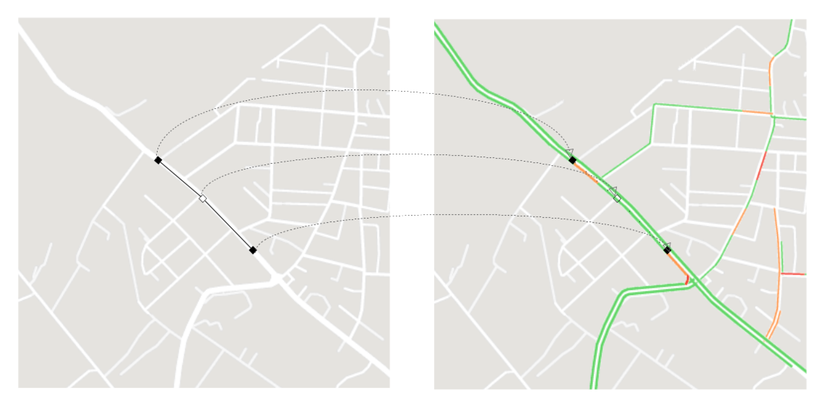
(derived from tags or default street type speed), geometry (pillar and tower nodes). The API provided from the GraphHopper project has been used to accomplish tasks as OSM importation, road graph generation and routing between customers. We extended this time-invariant graph representation by assigning a traffic profile only to time-dependent arcs. In particular, traffic data were obtained through a two step procedure. Firstly, given the geographic coordinates of two points at a specific zoom level, we defined a bounding box around the reference Earth area. Therefore, at the start of every time slot
h we captured a snapshot of the current map viewport augmented with the real-time traffic layer. Next, for each arc
belonging in the bounding box we subdivided its geometry in uniform length segments. We denoted the set of all segments endpoints for arc
by
. For each point
we projected the geographic coordinates over a pixel
of the image plane (
Figure 1). We used the Haversine formula to measure Earth distances. For each period
h the pixel
can assume a different color in the corresponding
h-th snapshot. The color is classified using the CIEDE2000 color distance [
40] from some reference color with a preassigned traffic jam factor as showed in
Table 1.
If did not belong to a street, we started a neighborhood exploration procedure in order to identify the nearest valid color. This task is executed to repair small alignment errors between the osm map and the traffic layer image. After classification, the traffic jam factor of arc was computed as the mean of the jam factors associated to each geographical point . An arc was deemed to be time-dependent if it had at least one traffic jam factor strictly lower than 1 in the time horizon.
4.2. Parameter Tuning
We have performed a preliminary tuning with the aim to select the most appropriate combination of parameters:
Table 2 summarizes the investigated values for each parameter.
Our datasets contained approximately 6–700 instances with 50 customers each: has been assigned to the training set, while the remaining to the test set. The best results, in terms of strength of captured relationships, were obtained by the following neural network settings: three layers, hyperbolic tangent activation function, five neurons in the hidden layer, LBFGS solver and constant learning rate.
As far as customer aggregation is concerned, it was necessary to project customers locations to a new planar reference system. According to the EPSG projection, we used the Transverse Mercator Projection for London and the Lambert Zone II Projection for Paris.
For London, 8 clusters gave the best results in terms of coefficient of determination (
), whilst for Paris 6 zones were the best case for neural network performance.
Table 3 and
Table 4 summarize the neural network mean errors (in minutes) for each zone. The
scores (=0.53 for the London instances and =0.60 for the Paris instances) suggest a moderate effect size.
4.3. Computational Results
The computational results are presented in
Table 5 and
Table 6. For each of the two testsets, we report:
the name of the test instance,
the objective value in minutes of the NNP solution,
the objective value in minutes of the ML-NNP solution,
the percentage of improvement of with respect to .
In our implementations, the maximum running time of both algorithms is only a few seconds or even a fraction of a second. Therefore we prefer not to report these figures. As shown in
Table 5 and
Table 6, the overall average improvement of ML-NNP over NNP is
for London, while
for Paris. It is worth noting that in the worst case ML-NNP gives the same performance of NNP, while in the best case can produce a solution with an improvement up to
(more than 70 min over a typical working day of 8 h).


