A Study of Ising Formulations for Minimizing Setup Cost in the Two-Dimensional Cutting Stock Problem

Abstract

We proposed the method that translates the two-dimensional CSP for minimizing the number of cuts to the Ising model. After that, we conducted computer experiments of the proposed model using the benchmark problem. From the above, the following results are obtained. (1) The proposed Ising model adequately represents the target problem. (2) Acceptance rates were as low as 0.2% to 9.8% and from 21.8% to 49.4%. (3) Error rates from optimal solution were as broad as 0% to 25.9%. For future work, we propose the following changes: (1) Improve the Hamiltonian for constraints. (2) Improve the proposed model to adjust more complex two-dimensional CSP and reduce the number of spins when it deals with large materials and components. (3) Conduct experiments using a quantum annealer.

1. Introduction

In several industries, such as paper, steel, and textile, items of specified sizes are cut out from the raw material placed on a flat surface. Problems aimed at minimizing the cost of such cutting work are referred to as two-dimensional cutting stock problems (CSPs) and two-dimensional bin packing problems (BPP), on which several studies have been carried out so far.

In particular, when positioning the items to be cut from raw material of fixed width W and variable height H, if the purpose of the problem is to minimize the height H, it is formulated as the strip packing problem (SPP), and various heuristic solutions have been proposed. E.G. Coffman Jr. et al. proposed the typical solution method, the first-fit decreasing height (FFDH) method and the next-fit decreasing height (NFDH) method [1]; C. M. Valenzuela et al. arranged FFDH and proposed the best-fit decreasing height (BFDH) method [2]; A. Lodi, et al., also arranged FFDH and proposed the floor–ceiling no rotation (FCNR) method [3]. B. Baker et al., in addition to the FFDH method, proposed solutions including the bottom-left method [4], in which items are introduced from the upper right of a material and then stacked from the bottom left, and heuristic approaches such as the bottom-left fill method [5], which adds an algorithm for reducing the gap between items. There are also solutions proposed using a metaheuristic method, such as the hill-climbing method [6], which is a typical local search method; simulated annealing [7]; the genetic algorithm (GA) [8,9,10]; and the native evolution algorithm [11], which eliminates GA crossover and evolves only by mutation. The SPP and BPP presume that all members have been arranged as a precondition; however, solutions [12] have been proposed using a knapsack problem approach when not all members have been arranged for selecting members that are given gain so that their sum is maximized, although many of these deal with materials as cost objects. These previous studies are aimed at maximizing the yield of raw materials as the cost target.

However, it is not just the material cost that must be considered [13]. For example, at a manufacturing site where special sheet-like materials are cut, a setup change cost is incurred for each cutting, which significantly impacts the total cost. Hence, a technique that can facilitate a reduction of the setup change cost is desired. In this paper, we propose an allocation method aimed at minimizing the number of setup changes by applying conventional methods, such as the FFDH and binary tree methods, for manufacturing sites that cut special sheet-like material. This method has helped achieve a reduction in the number of setup changes while ensuring a high yield [14].

Because a two-dimensional CSP is considered $\mathcal{N}\mathcal{P}$-hard, combinatorial explosion occurs when the complexity of the problem and, in turn, the scale of the solutions increases, leading to an exponential increase in the calculation time. In contrast, the actual problem represented by the two-dimensional CSP has a short lead time and requires a high-speed solution.

Quantum computers are next-generation computers that use quantum mechanics and are implemented through two types of methods: the quantum annealing and quantum gate methods. The quantum annealer is considered to be suitable for solving combinatorial optimization problems. Therefore, various combinatorial optimization problems have been studied using quantum annealing. In a previous study on the BPP, Terada et al. (2018) performed Ising modeling using sequence pairs for maximizing the yield of the rectangular packing problem [15]. Furthermore, Kida et al. (2000) performed Ising modeling with a formulation based on the NFDH method for the glass processing industry; they compared the performances of the quantum annealer and the classical bifurcation machine [16]. However, Ising models aimed at reducing setup change cost (= number of cuts) in the two-dimensional CSP have not yet been created.

Therefore, in this study, we propose an Ising model for the two-dimensional CSP that minimizes the number of cuts, we perform simulation experiments on benchmark problems, and we compare the results with the optimal solution determined using a solver [17].

2. Ising Model

When solving a combinatorial optimization problem using a quantum annealer, it is necessary to transform it into an equation referred to as the Ising model. The Ising model is a statistical mechanics model that represents the properties of a magnetic material, and the state of the magnetic material is evaluated by calculating the upward or downward state of the spin. Spin has two forces: a local field that acts only on that spin, and an interaction that acts on the connected spins. The state of the spin is updated by these forces so that the total energy is stabilized.

When the entire system is in the most stable state, the Hamiltonian $\mathcal{H}$, which represents the total energy of the Ising model, is the minimum (ground state). Equation (1) expresses this Hamiltonian. Here, it should be noted that $s_i \mathrm{and} s_j$ are the directions (±1) of the spins $i \mathrm{and} j$, respectively, $J_{ij}$ represents the interaction, $h_i$ is the local field of spin $i$, $E$ is the number of edges, and $V$ is the number of spins:

$$\mathcal{H}={\displaystyle \sum }_{\left(i,j\right)\in E}{J}_{ij}{s}_i{s}_j-{\displaystyle \sum }_{i\in V}{h}_i{s}_i$$

(1)

3. Target Overview

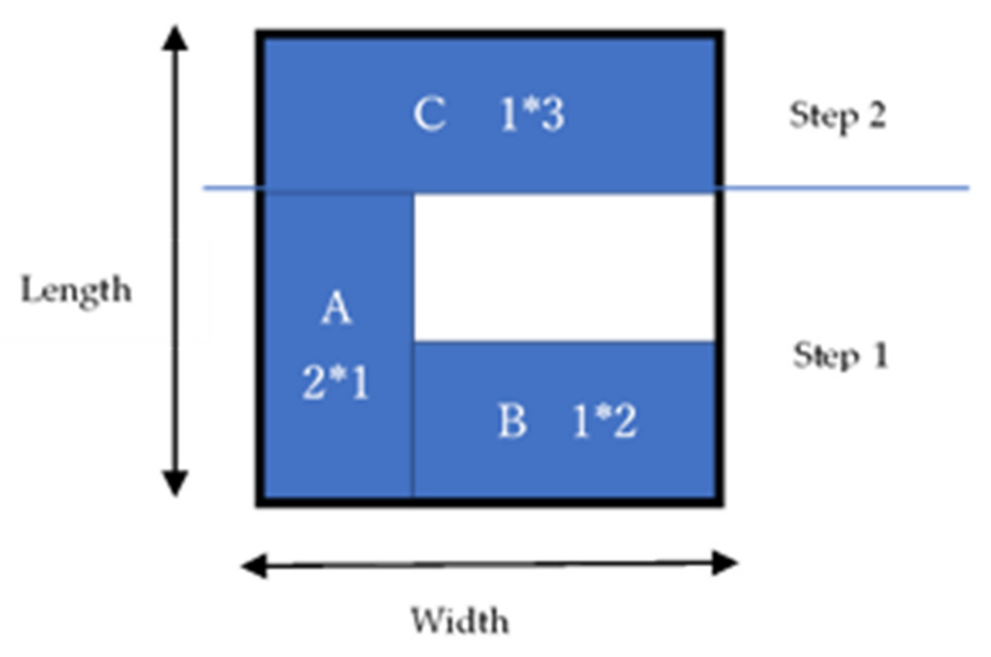
We consider a two-dimensional CSP as the target problem. However, if applied as it is, the number of spins in the quantum annealer may be insufficient, as there are several constraints. Hence, some simplification is required. Figure 1 presents an example of the allocation and specific conditions.

The main conditions of this model are as follows:

• There are infinite base materials with fixed widths and lengths.
• The items shall be allocated from the lower left of the base material.
• The allocated items must not protrude from the base material.
• The allocated items must not overlap.
• All the items are allocated from one of the base materials only once.
• The items must not be rotated.
• Allocation in the vertical direction of the base material is known as a step, and the length of each step is the length of the longest piece in that step.
• Items shall not be allocated vertically in each step.
• If there are two or more items of the same length in each step, their horizontal cutting is carried out all at once.
• If the allocated piece in each base material touches the upper side of the base material, horizontal cutting is omitted.
• If the total width of the items allocated in each step matches the width of the base material, the vertical cutting of the rightmost piece is omitted.

4. Ising Modeling

Table 1. List of variables.

Symbol	Description
$Bin\_H$	Length of base material
$Bin\_W$	Width of base material
$I$	Number of base materials
$i$	$\mathrm{Base}\mathrm{material}\mathrm{number}(i=1,\dots ,I$)
$j$	$\mathrm{Number}\mathrm{of}\mathrm{vertical}\mathrm{steps}\mathrm{in}\mathrm{base}\mathrm{material}(j=1,\dots ,Bin\_H$)
$K$	Number of items
$k$	$\mathrm{Piece}\mathrm{number}(k=1,\dots ,K$)
$l$	Spin number representing total width of items $(l=0,\dots ,Bin\_W$)
$m$	Spin number representing longest piece length $(m=0,\dots ,Bin\_H$)
$n$	Spin number representing type of piece length $(n=1,\dots ,Bin\_H$)
$p$	$\mathrm{Spin}\mathrm{number}\mathrm{representing}\mathrm{total}\mathrm{length}\mathrm{of}\mathrm{longest}\mathrm{items}(p=0,\dots ,Bin\_H$)
$h_k$	Length of piece k
$w_k$	Width of piece k
${\mathcal{H}}_{Hcut}$	Hamiltonian representing number of horizontal cuts in base material
${\mathcal{H}}_{Wcut}$	Hamiltonian representing number of vertical cuts in base material
${\mathcal{H}}_A$	Hamiltonian for piece allocation
${\mathcal{H}}_H$	Hamiltonian representing vertical allocation constraint of a piece
${\mathcal{H}}_W$	Hamiltonian representing horizontal allocation constraint of a piece
${\mathcal{H}}_{Htype}$	Hamiltonian to obtain piece length type at each step
${\mathcal{H}}_{Hlongest}$	Hamiltonian to ensure that the longest piece in each step is indeed the longest
$\sigma$	Objective function parameters
${\lambda }_A$	${\mathcal{H}}_A$ parameters
${\lambda }_H,{\mu }_H$	${\mathcal{H}}_H$ parameters
${\lambda }_W,{\mu }_W$	${\mathcal{H}}_W$ parameters
${\sigma }_t$	${\mathcal{H}}_{Htype}$ parameters
${\sigma }_l,{\lambda }_l$	${\mathcal{H}}_{Hlongest}$ parameters

lists the variables used in this paper. Furthermore, there are five types of spins as follows:

$$s_{i,j,k}=\left\{\begin{array}{l}|1 \mathrm{P}\mathrm{i}\mathrm{e}\mathrm{c}\mathrm{e} k \mathrm{i}\mathrm{s} \mathrm{a}\mathrm{l}\mathrm{l}\mathrm{o}\mathrm{c}\mathrm{a}\mathrm{t}\mathrm{e}\mathrm{d} \mathrm{t}\mathrm{o} j\mathrm{t}\mathrm{h} \mathrm{s}\mathrm{t}\mathrm{e}\mathrm{p} \mathrm{o}\mathrm{f} \mathrm{b}\mathrm{a}\mathrm{s}\mathrm{e} \mathrm{m}\mathrm{a}\mathrm{t}\mathrm{e}\mathrm{r}\mathrm{i}\mathrm{a}\mathrm{l} i\\ |0 \mathrm{O}\mathrm{t}\mathrm{h}\mathrm{e}\mathrm{r}\mathrm{w}\mathrm{i}\mathrm{s}\mathrm{e}\end{array}\right.$$

$$s{w}_{i,j,l}=\left\{\begin{array}{l}|1 \mathrm{T}\mathrm{o}\mathrm{t}\mathrm{a}\mathrm{l} \mathrm{w}\mathrm{i}\mathrm{d}\mathrm{t}\mathrm{h} \mathrm{o}\mathrm{f} \mathrm{i}\mathrm{t}\mathrm{e}\mathrm{m}\mathrm{s} \mathrm{a}\mathrm{l}\mathrm{l}\mathrm{o}\mathrm{c}\mathrm{a}\mathrm{t}\mathrm{e}\mathrm{d} \mathrm{t}\mathrm{o} j\mathrm{t}\mathrm{h} \mathrm{s}\mathrm{t}\mathrm{e}\mathrm{p} \mathrm{o}\mathrm{f} \mathrm{b}\mathrm{a}\mathrm{s}\mathrm{e} \mathrm{m}\mathrm{a}\mathrm{t}\mathrm{e}\mathrm{r}\mathrm{i}\mathrm{a}\mathrm{l} i \mathrm{i}\mathrm{s} l \\ |0 \mathrm{O}\mathrm{t}\mathrm{h}\mathrm{e}\mathrm{r}\mathrm{w}\mathrm{i}\mathrm{s}\mathrm{e}\end{array}\right.$$

$$s{h}_{i,j,m}=\left\{\begin{array}{l}|1 \mathrm{L}\mathrm{o}\mathrm{n}\mathrm{g}\mathrm{e}\mathrm{s}\mathrm{t} \mathrm{p}\mathrm{i}\mathrm{e}\mathrm{c}\mathrm{e} \mathrm{i}\mathrm{n} j\mathrm{t}\mathrm{h} \mathrm{s}\mathrm{t}\mathrm{e}\mathrm{p} \mathrm{o}\mathrm{f} \mathrm{b}\mathrm{a}\mathrm{s}\mathrm{e} \mathrm{m}\mathrm{a}\mathrm{t}\mathrm{e}\mathrm{r}\mathrm{i}\mathrm{a}\mathrm{l} i \mathrm{i}\mathrm{s} m\\ |0 \mathrm{O}\mathrm{t}\mathrm{h}\mathrm{e}\mathrm{r}\mathrm{w}\mathrm{i}\mathrm{s}\mathrm{e}\end{array}\right.$$

$$sh{c}_{i,j,n}=\left\{\begin{array}{l}|1 \mathrm{P}\mathrm{i}\mathrm{e}\mathrm{c}\mathrm{e} \mathrm{o}\mathrm{f} \mathrm{l}\mathrm{e}\mathrm{n}\mathrm{g}\mathrm{t}\mathrm{h} n \mathrm{i}\mathrm{s} \mathrm{a}\mathrm{l}\mathrm{l}\mathrm{o}\mathrm{c}\mathrm{a}\mathrm{t}\mathrm{e}\mathrm{d} \mathrm{i}\mathrm{n} j\mathrm{t}\mathrm{h} \mathrm{s}\mathrm{t}\mathrm{e}\mathrm{p} \mathrm{o}\mathrm{f} \mathrm{b}\mathrm{a}\mathrm{s}\mathrm{e} \mathrm{m}\mathrm{a}\mathrm{t}\mathrm{e}\mathrm{r}\mathrm{i}\mathrm{a}\mathrm{l} i\\ |0 \mathrm{O}\mathrm{t}\mathrm{h}\mathrm{e}\mathrm{r}\mathrm{w}\mathrm{i}\mathrm{s}\mathrm{e}\end{array}\right.$$

$$sh{t}_{i,p}=\left\{\begin{array}{l}|1 \mathrm{T}\mathrm{o}\mathrm{t}\mathrm{a}\mathrm{l} \mathrm{l}\mathrm{e}\mathrm{n}\mathrm{g}\mathrm{t}\mathrm{h} \mathrm{o}\mathrm{f} \mathrm{l}\mathrm{o}\mathrm{n}\mathrm{g}\mathrm{e}\mathrm{s}\mathrm{t} \mathrm{i}\mathrm{t}\mathrm{e}\mathrm{m}\mathrm{s} \mathrm{o}\mathrm{f} \mathrm{e}\mathrm{a}\mathrm{c}\mathrm{h} \mathrm{s}\mathrm{t}\mathrm{e}\mathrm{p} \mathrm{o}\mathrm{f} \mathrm{b}\mathrm{a}\mathrm{s}\mathrm{e} \mathrm{m}\mathrm{a}\mathrm{t}\mathrm{e}\mathrm{r}\mathrm{i}\mathrm{a}\mathrm{l} i \mathrm{i}\mathrm{s} p\\ |0 \mathrm{O}\mathrm{t}\mathrm{h}\mathrm{e}\mathrm{r}\mathrm{w}\mathrm{i}\mathrm{s}\mathrm{e}\end{array}\right.$$

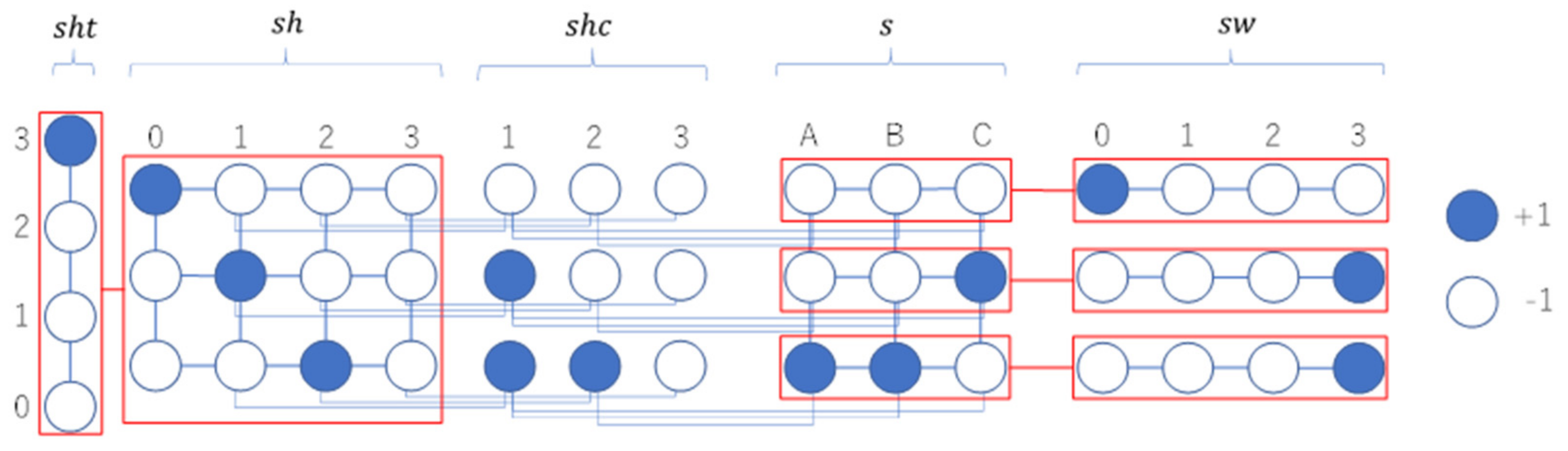
Figure 2 is an example of relations about the five kinds of spins. It shows the set of the spin of Figure 1. And the spin sets in the frame have mutual interaction with connected spins. The spin sets in the line frame have mutual interaction under the constraint condition.

The full Hamiltonian of the proposed Ising model is expressed as follows:

$$\mathcal{H}={\mathcal{H}}_{Hcut}+{\mathcal{H}}_{Wcut}+{\mathcal{H}}_A+{\mathcal{H}}_H+{\mathcal{H}}_W+{\mathcal{H}}_{Hlongest}+{\mathcal{H}}_{Htype}$$

(2)

where ${\mathcal{H}}_{Hcut} \mathrm{and}{\mathcal{H}}_{Wcut}$ are Hamiltonians that represent objective functions and ${\mathcal{H}}_A, {\mathcal{H}}_H,{\mathcal{H}}_W, {\mathcal{H}}_{Hlongest,} \mathrm{and}{\mathcal{H}}_{Htype}$ are Hamiltonians that represent constraints. ${\mathcal{H}}_{Hcut}\mathrm{and}{\mathcal{H}}_{Wcut}$ are represented as follows:

$${\mathcal{H}}_{Hcut}=\sigma {\displaystyle \sum }_{i=1}^I\left({\displaystyle \sum }_{j,n=1}^{Bin\_H}sh{c}_{i,j,n}-sh{t}_{i,Bi{n}_H}\left(1-sh{t}_{i,0}\right)\right)$$

(3)

$${\mathcal{H}}_{Wcut}=\sigma {\displaystyle \sum }_{i=1}^I{\displaystyle \sum }_{j=1}^{Bin\_H}\left({\displaystyle \sum }_{k=1}^K{s}_{i,j,k}-s{w}_{i,j,Bi{n}_W}\left(1-s{w}_{i,j,0}\right)\right)$$

(4)

Equation (3) represents the number of cuts in the horizontal direction and satisfies Constraints 9 and 10 listed in Section 3. For each piece length type at each step, the number of cuts is incremented, and when the sum of lengths of the longest items at each step matches the length of the base material, the number of cuts is omitted once.

Equation (4) expresses the number of cuts in the vertical direction and satisfies Constraint 11 listed in Section 3. The number of cuts is incremented for each piece at each step, and when the total width of the items allocated to each step matches the width of the base material, the number of cuts is omitted once.

${\mathcal{H}}_A$ is expressed as follows:

$${\mathcal{H}}_A={\lambda }_A{\left({\displaystyle \sum }_{i=1}^I{\displaystyle \sum }_{j=1}^{Bin\_H}{s}_{i,j,k}-1\right)}^2 \forall k$$

(5)

Equation (5) expresses a constraint on the number of times items allocated, and satisfies Constraint 5 listed in Section 3. Its value is the lowest when all the items are allocated to one of the base materials only once.

${\mathcal{H}}_H \mathrm{and}{\mathcal{H}}_W$ are expressed as follows:

$${\mathcal{H}}_H={\lambda }_H{\left(1-{\displaystyle \sum }_{p=0}^{Bin\_H}sh{t}_{i,p}\right)}^2+{\mu }_H{\left({\displaystyle \sum }_{p=0}^{Bin\_H}p\cdot sh{t}_{i,p}-{\displaystyle \sum }_{j=1,m=0}^{Bin\_H}m\cdot s{h}_{i,j,m}\right)}^2\forall i$$

(6)

$${\mathcal{H}}_W={\lambda }_W{\left(1-{\displaystyle \sum }_{l=0}^{Bin\_H}s{w}_{i,j,l}\right)}^2+{\mu }_W{\left({\displaystyle \sum }_{l=0}^{Bin\_W}l\cdot s{w}_{i,j,l}-{\displaystyle \sum }_{k=1}^K{w}_k\cdot s_{i,j,k}\right)}^2\forall i,j.$$

(7)

Equation (6) represents the constraint for preventing the items from protruding vertically from the base material, and its value is the lowest when there is only one spin with $sht=1$ in each base material and the subscript $p$ of the spin with $sht=1$ matches the sum of the subscripts $m$ of the$sh$at each step.

Equation (7) expresses the constraint for preventing the items from protruding horizontally from the base material, and its value is the lowest when there is only one spin with $sw=1$ at each step for each base material, and the subscript $l$ of the spin with $sw=1$ matches the total width of the items allocated to the target step.

Equations (6) and (7) satisfy Condition 3 listed in Section 3. ${\mathcal{H}}_{Htype}$ is expressed as follows:

$${\mathcal{H}}_{Htype}=-{\sigma }_t{\displaystyle \sum }_{n=1}^{Bin\_H}\left(1-sh{c}_{i,j,n}\right)\left(1-2{\displaystyle \sum }_{k|h_k=n}{s}_{i,j,k}\right)\forall i,j$$

(8)

Although Equations (3)–(7) can be used to represent a two-dimensional CSP that minimizes the number of cuts, the spin $shc$ cannot always correctly represent the piece length type at each step. Therefore, a constraint is set on $shc$ by Equation (8). This equation yields the minimum value when the values of all the variables $s_{i,j,k}$ with $h_k=n$ become 0 at each step for each base material, leading to $shc=0$, and when one of these values becomes 1, leading to $shc=1$.

${\mathcal{H}}_{Hlongest}$ is expressed as follows:

$${\mathcal{H}}_{Hlongest}={\lambda }_l{\left(1-{\displaystyle \sum }_{m=0}^{Bin\_H}s{h}_{i,j,m}\right)}^2-{\sigma }_l{\displaystyle \sum }_{n=1}^{Bin\_H}n\cdot sh{c}_{i,j,n}s{h}_{i,j,m|m=n} \forall i,j$$

(9)

Similar to $shc$, the spin $sh$ cannot always correctly represent the longest piece at each step only through Equations (3)–(8). Therefore, a constraint is set on $sh$ by Equation (9). This equation yields the minimum value only when the$sh$with the subscript $m$ that matches the longest of the items allocated at each step for each base material becomes 1.

5. Computer Experiment

• Experimental conditions

To confirm the validity of the proposed Ising model, we performed a computer experiment. Because the target problem is a benchmark problem [18], it is considered as an instance that satisfies the conditions specified in

Table 2. Experimental conditions for the benchmark problem.

Name	Value
$Bin\_H$	10
$Bin\_W$	10
$K$	20

.

However, for the sake of simplicity, the length of the base material $Bin\_H$ is considered as a variable, and it is assumed that a cut is always made in line with the longest piece among the allocated items. Thus, the full Ising model of this experiment is represented by Equation (10):

$$\mathcal{H}={\mathcal{H}}_{Hcut}+{\mathcal{H}}_{Wcut}+{\mathcal{H}}_A+{\mathcal{H}}_W+{\mathcal{H}}_{Htype}$$

(10)

For the experiment, Equation (10) is converted into a QUBO matrix, which is known to have a one-to-one correspondence with the Ising model. The QUBO matrix is applied to QBsolv and neal. QBsolv can optimize calculations through tabu search, and neal can optimize calculation using simulated annealing [19].

Table 3. Parameter settings.

Variable Identifier	Value
$\sigma$	1000
${\sigma }_t$	5000
${\lambda }_A$	500,000
${\lambda }_W$	500,000
${\mu }_W$	10,000
Number of trials	1000

shows each parameter setting that was set by the preliminary experiment.

Under these experimental conditions, the number of logical spins are $s_{i,j,k} 10\times 10\times 20=2000$, $s{w}_{i,j,l}:11\times 10\times 20=2200$, $s{h}_{i,j,m}:11\times 10\times 20=2200$, $sh{c}_{i,j,n}:10\times 10\times 20=2000$ and $sh{t}_{i,p}:11\times 20=220$. Since $s{w}_{i,j,l}$ and $s{h}_{i,j,m}$ need a spin to express height 0, these needs 11 spins for height.

Regarding the computer environments, Intel(R) Core(TM) i7-7700HQ CPU, 2.8 GHz, RAM 16 GB, and a programing is used Python.

• Experimental results

We now consider the acceptance rate and accuracy of the experimental results. Furthermore, we calculate the optimal solution of the target benchmark problem using Google OR-tools [20] and compare the two optimizer’s results.

Table 4. Comparison of the experimental results obtained using QBsolv and the optimal solution.

No.	Best Value	Acc. Rate	Av.	Var.	SD	Opt.
1	35	3.2	37.688	1.152	1.073	32
2	34	5.7	37.702	1.613	1.270	29
3	35	0.7	37.000	1.143	1.069	34
4	34	3.1	37.839	1.361	1.167	27
5	34	0.9	34.889	0.321	0.567	31
6	34	0.2	35.000	1.000	1.000	31
7	34	2.7	37.370	1.048	1.024	27
8	35	9.8	38.622	1.357	1.165	28
9	32	1.0	36.900	3.090	1.758	32
10	35	0.9	36.778	1.284	1.133	28

and

Table 5. Comparison of the experimental results obtained using neal and the optimal solution.

No.	Best Value	Acc. Rate	Av.	Var.	SD	Opt.
1	34	36.3	37.788	1.164	1.079	32
2	34	42.4	37.807	1.081	1.039	29
3	34	26.2	37.206	0.706	0.840	34
4	34	40.0	37.800	1.040	1.020	27
5	32	27.3	35.150	0.824	0.908	31
6	33	21.8	35.459	0.459	0.678	31
7	34	46.3	37.659	1.110	1.054	27
8	34	49.4	38.690	1.340	1.160	28
9	34	30.5	37.230	0.774	0.880	32
10	32	26.5	36.758	1.157	1.076	28

indicate that the relative error between the best solution using the proposed Ising model and the optimal solution using Google OR-tools were 0–25.9%, respectively, obtained using both QBsolv and neal. The calculation times are from 0.0 to 3.0 s in all instances. The optimal solutions were obtained in Instances 9 and 3 in QBsolv and neal, respectively. The acceptance rates were 0.2–9.8% and 21.8–49.4%, respectively. The difference in the acceptance rate is the algorithmic difference in each optimizer. As neal used SA, the acceptance rate of the average became higher because the acceptance rate of the initial search was high. About QBsolv, several solutions that violated the constraints were calculated. These optimizers are high-performance, but there is little room for parameter adjustment. For the improvement of the solution, the parameters can be adjusted or the spin’s design of the Ising model can be modified. Although the parameters ${\mathcal{H}}_{Htype}$ and ${\mathcal{H}}_{Hlongest}$ of the Ising model are constraints, their minimum values change depending on the problem and other parameters, and they are effectively objective functions that impose constraints on other parameter settings. If a model could be constructed such that the values of these Hamiltonians could reach a minimum of 0, the range of acceptable values for the other parameters would become wider, and flexible response would become possible.

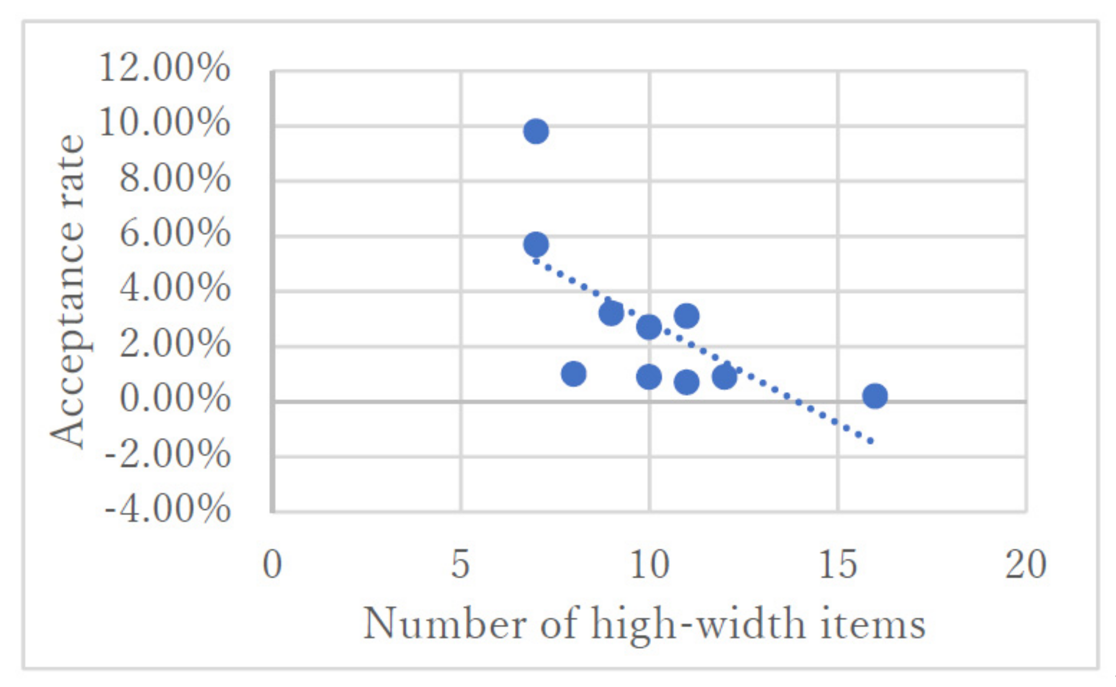
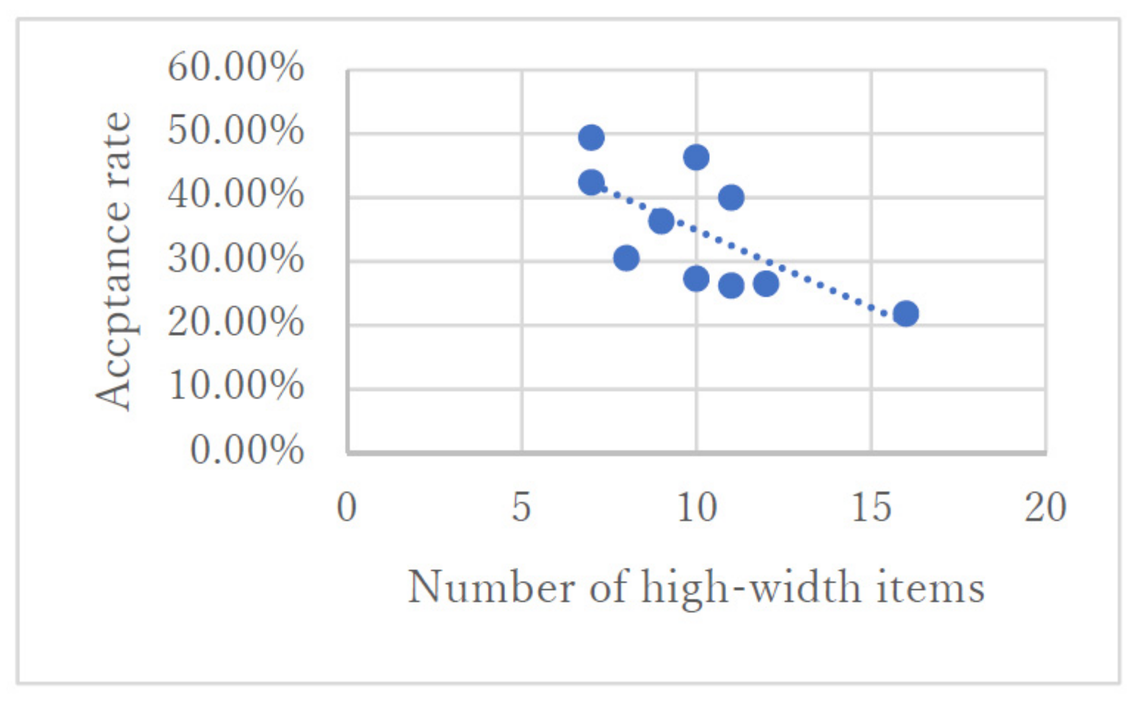
Further, the reason for the difference in the acceptance rate depending on the instance, is that if the number of items with widths exceeding 50% of the width of the base material (number of high-width items) is high, the ratio of the solution space to the search space becomes small. The probability of obtaining an acceptable solution within the execution time becomes low. Figure 3 and Figure 4 present the distribution maps of the acceptance rates and the numbers of high-width items at each instance obtained using QBsolv and neal, respectively. The broken lines in the figures represent the linear approximation curves. These figures indicate that the acceptance rate of the solution decreases proportionally with the number of high-width items.

6. Conclusions

In this paper, we propose an Ising model with the aim to minimizing the number of cuts in a two-dimensional CSP. This is first trying a formulation of a Ising model. In this study, five kinds of spins are prepared, and these change their state with interaction. The proposed Ising model worked appropriately, and as the number of cuts decreased, the energy consumed also reduced. However, in the experiment, the acceptance rates were 0.2–9.8% for QBsolv and 21.8–49.4% for neal. The relative error of the optimal solution was 0–25.9%, which indicates a wide range. Although the relative errors are depend on an instance condition, the parameter setting and the Ising modeling have to improve for versatility. When minimum value of parameters regarding Hamiltonian ${\mathcal{H}}_{Htype}$ and ${\mathcal{H}}_{Hlongest}$ become 0, the other parameter’s values are able to change more flex. Furthermore, in the proposed method, the constraints for the allocation of items in the vertical and horizontal directions were realized by preparing spins based on the size of the base material. However, as the size of the base material increases, the number of spins to be secured also increases, making it difficult to apply to the quantum annealer. The following can be listed as future challenges:

• Improving the constraints used in the Ising model;
• Adjusting the parameters further;
• Considering the omission of vertical cutting;
• Devising an Ising model that can be applied to situations that use large-sized base materials;
• Application to the quantum annealer.

References

- Coffman, E.G., Jr.; Garey, M.R.; Johnson, D.S.; Tarjan, R.E. Performance bounds for level oriented two-dimensional packing algorithms. SIAM J. Comput. 1980, 9, 808–826. [Google Scholar] [CrossRef]
- Mumford-Valenzuela, C.L.; Vick, J.; Wang, P.Y. Heuristic for Large Strip Packing Problems with Guillotine Patterns: An Empirical Study. In Proceedings of 4th Metaheuristics: Computer Decision-Making, Applied Optimization; Springer: Boston, MA, USA, 2003; pp. 501–522. [Google Scholar]
- Lodi, A.; Martello, S.; Vigo, D. Neighborhood Search Algorithm for the Guillotine Non-Oriented Two-Dimensional Bin Packing Problem. In Meta-Heuristics: Advances and Trends in Local Search Paradigms for Optimization; Voss, S., Martello, S., Osman, I.H., Roucairol, C., Eds.; Kluwer Academic Publishers: Boston, MA, USA, 1998; pp. 125–139. [Google Scholar]
- Baker, B.S.; Coffman, E.G., Jr.; Rivest, R.L. Orthogonal packing in two dimensions. SIAM J. Comput. 1980, 9, 846–855. [Google Scholar] [CrossRef]
- Chazelle, B. The bottom-left bin-packing heuristic: An efficient implementation. IEEE Trans. Comput. 1983, c-32, 697–707. [Google Scholar] [CrossRef]
- Lewi, R. A General-Purpose Hill-Climbing Method for Order Independent Minimum Grouping Problems: A Case Study in Graph Coloring and Bin Packing. Comput. Oper. Res. 2009, 36, 2295–2310. [Google Scholar]
- Rao, R.L.; Iyengar, S.S. Bin-packing by simulated annealing. Comput. Math. Appl. 1994, 27, 71–82. [Google Scholar] [CrossRef] [Green Version]
- Falkenauer, E. A hybrid grouping genetic algorithm for bin packing. J. Heuristics 1996, 2, 5–30. [Google Scholar] [CrossRef] [Green Version]
- Mohamadi, N. Application of Genetic Algorithm for the Bin Packing Problem with a New Representation Scheme. Math. Sci. 2010, 4, 253–266. [Google Scholar]
- Laabadi, S.; Naimi, M.; El Amri, H.; Achchab, B. A Crow Search-Based Genetic Algorithm for Solving Two-Dimensional Bin Packing Problem. In Joint German/Austrian Conference on Artificial Intelligence; Springer: Cham, Switzerland, 2019; pp. 203–215. [Google Scholar]
- Hopper, E.; Turton, B.C.H. An empirical investigation of meta-heuristic and heuristic algorithms for a 2D packing problem. Eur. J. Oper. Res. 2001, 128, 34–57. [Google Scholar] [CrossRef]
- Bidhu, B.M.; Kamlesh, M.; Nancy, J.I. Value considerations in three-dimensional packing—A heuristic procedure using the fractional knapsack problem. Eur. J. Oper. Res. 1994, 74, 143–151. [Google Scholar]
- Umetani, S. Formulation and Approximate Solution for the Cutting Stock Problem Considering the Minimization of the Number of Setup Changes; Research Institute for Mathematical Sciences (RIMS) Kokyuroku: Kyoto, Japan, 1999; Volume 1114, pp. 233–241. [Google Scholar]
- Arai, H.; Haraguchi, H. Solution approaches for the two-dimensional cutting stock problem. In Proceedings of the 64th System Control Information Society Research, Online, 20 May 2020. [Google Scholar]
- Terada, K.; Oku, D.; Kanamaru, S.; Tanaka, S.; Hayashi, M.; Yamaoka, M.; Yanagisawa, M.; Togawa, N. An Ising model mapping to solve rectangle packing problem. In Proceedings of the 2018 International Symposium on VLSI Design, Automation and Test (VLSI-DAT), Hsinchu, Taiwan, 16–19 April 2018. [Google Scholar]
- Kida, T.; Tonoue, R.; Yazane, T.; Tatekawa, M.; Katsuki, R. Application of Ising machine to optimize glass-plate cutting patterns with guillotine-cut constraint. AGC Res. Rep. 2020, 70, 12–17. [Google Scholar]
- Arai, H.; Haraguchi, H. Ising formulations for the two-dimensional cutting stock problem with setup cost. arXiv 2021, arXiv:2103.16796. [Google Scholar]
- Available online: http://or.dei.unibo.it/library/two-dimensional-bin-packing-problem (accessed on 29 January 2021).
- Available online: https://developers.google.com/optimization (accessed on 26 February 2021).
- Available online: https://github.com/dwavesystems/dwave-ocean-sdk (accessed on 26 February 2021).
Figure 1.
Example of allocation.
Figure 2.
Relations of the spins (Figure 1).
Figure 3.
Distribution of the acceptance rates obtained using QBsolv at each instance and the numbers of high-width items at those instances.
Figure 4.
Distribution of the acceptance rates obtained using neal at each instance and the numbers of high-width items at those instances.