
Mechanical Fault Prognosis through Spectral Analysis of Vibration Signals


1
Computer and Information Security Department, Zhejiang Police College, Hangzhou 310018, China
2
School of Automation, Zhejiang Institute of Mechanical & Electrical Engineering, Hangzhou 310059, China
3
Department of Electrical and Electronic Engineering, Southern University of Science and Technology, Shenzhen 518055, China
4
Department of Electrical and Computer Engineering, Concordia University, Montreal, QC H3G 2W1, Canada
*
Author to whom correspondence should be addressed.
Algorithms 2022, 15(3), 94; https://0-doi-org.brum.beds.ac.uk/10.3390/a15030094
Submission received: 5 February 2022
/
Revised: 8 March 2022
/
Accepted: 14 March 2022
/
Published: 15 March 2022
(This article belongs to the Special Issue 1st Online Conference on Algorithms (IOCA2021))
Abstract
:Vibration signal analysis is the most common technique used for mechanical vibration monitoring. By using vibration sensors, the fault prognosis of rotating machinery provides a way to detect possible machine damage at an early stage and prevent property losses by taking appropriate measures. We first propose a digital integrator in frequency domain by combining fast Fourier transform with digital filtering. The velocity and displacement signals are, respectively, obtained from an acceleration signal by means of two digital integrators. We then propose a fast method for the calculation of the envelope spectra and instantaneous frequency by using the spectral properties of the signals. Cepstrum is also introduced in order to detect the unidentifiable periodic signal in the power spectrum. Further, a fault prognosis algorithm is presented by exploiting these spectral analyses. Finally, we design and implement a visualized real-time vibration analyzer on a Raspberry Pi embedded system, where our fault prognosis algorithm is the core algorithm. The real-time signals of acceleration, velocity, displacement of vibration, as well as their corresponding spectra and statistics, are visualized. The developed fault prognosis system has been successfully deployed in a water company.
1. Introduction
Vibration has been an important direction in industry. The operating condition of industrial equipment is closely related to vibration. The primary goal of vibration-based machine condition monitoring is to avoid catastrophic machine failures that can lead to secondary damage, shutdown, potential safety accidents, production losses, high maintenance costs, and more. Based on the collision vibration signal between the metal plate and coal gangue, a coal gangue recognition scheme in the top coal caving process is proposed in [1]. A vibration signal-based method is proposed in [2] for condition monitoring and fault diagnosis of the water-circulating heat exchangers used in the petrochemical industry. The vibration method is considered to be an economical and non-destructive method for exploring the operating conditions and assessing the mechanical integrity and performance of the transformer [3,4].
The causes of mechanical vibration are roughly explained as follows. Modern machinery cannot do without rolling bearings as an important transmission component. When the lubricating oil film ruptures due to various reasons, such as overload and insufficient oil, the local stress in the bearing area is too large, then the contact body will produce plastic hardening and cracks. As a result of repeated crushing, the cracks continue to expand, and the material will peel off from the contact body after expanding to a certain degree, forming pits. When the contact body passes a pit, due to an abrupt change in contact area, the bearing force will also change abruptly, resulting in a short impulse force. This impulse force is reflected in the vibration signal, which is the impulse response of a shock decay. The pits appear on the inner and outer rings of the bearing and the rolling element, generating impulse signals of different frequencies. In a vibration analyzer, how to detect these impulse frequencies from sensor signals is key to fault diagnosis of bearings.
There are many methods for processing vibration signals, which can be roughly divided into two categories. One is the traditional methods, typically amplitude domain analysis, Fourier transform, and correlation analysis. The amplitude domain analysis method is a time-domain analysis method that describes the amplitude variation with time, while the Fourier transform and correlation analysis are based on the time-domain statistical analysis. Generally, the research objects of these methods are stationary signals. The other category is modern methods, typically, variational mode decomposition [5], singular value decomposition [6], principal component analysis [7], filtering [8,9,10], Wigner–Ville distribution, spectral analysis [11], Hilbert–Huang transform [12], wavelet analysis [13,14], blind source separation, and higher order statistics analysis. They are widely used as they achieve good results for non-stationary signals.
Much of the literature combines traditional time-frequency domain analysis methods with machine learning, deep learning and artificial intelligence to propose many new approaches for vibration fault diagnosis [15,16,17,18,19,20,21,22]. Furthermore, the use of machine learning methods to analyze vibration data is expected to significantly reduce the associated analysis effort and further improve diagnostic accuracy [15]. In order to extract impulsive components precisely, an approach that combines K-clustering with singular value decomposition and split-Bregman is proposed in [16]. An that approach combines artificial neural network and support vector machine for identifying and measuring shaft misalignment under variable load conditions is proposed in [17]. By transforming raw vibration signals into images and using a convolutional neural network for classification, a deep learning-based fault classification model is proposed in [18]. In order to differentiate among faulty states, the authors in [19] investigated various multi-axis statistical features and employed K-Nearest Neighbors and Decision Trees to obtain a model. A refined composite multiscale dispersion entropy and deep belief network-extreme learning machine based sub-health recognition offline algorithm is proposed and optimized by an improved firework algorithm in [20]. For bearing fault detection, a new framework based on wavelet transform and discrete Fourier transform with deep learning is proposed in [21]. The chapter “Vibration-Based Condition Monitoring Using Machine Learning” in book [22] describes the fault-detection and -diagnosis framework, and provides many machine learning algorithms, such as unsupervised/semisupervised learning, reinforcement, and transfer learning.
However, machine learning requires huge amounts of valid data. The visualized real-time vibration analyzer designed in this paper stores the data sampled from measurements to a local database and uploads them to a server through a 5G network. The proposed analyzer provides an effective data source for machine learning. Meanwhile, it also has the traditional spectrum analysis function.
The main contributions of this paper are given as follows.
- A digital integrator in frequency domain is proposed by combining fast Fourier transform with digital filtering. The analyzer uses a vibration acceleration sensor to sample acceleration signal. The corresponding velocity and displacement signals are, respectively, obtained from the acceleration sensor signal by means of two digital integrations. Frequency-domain integration has higher accuracy, faster computation speed, and better stability than the time-domain integration;
- By using the spectral properties of the signals, a fast method for calculating the envelope spectrum and instantaneous frequency of the narrowband modulated signal is derived. In order to detect an unidentifiable periodic signal in the power spectrum, cepstrum is introduced. As a result, the analyzer can perform power spectrum, envelope spectrum, and cepstrum analysis simultaneously. Further, a fault prognosis algorithm is given by exploiting these spectral analyses;
- A Raspberry Pi-based analyzer with integrated vibration signal acquisition, analysis, display, data storage, and uploading is proposed. The application running on the Raspberry Pi uses TCP protocol to transmit to a remote server the raw vibration data that the fault prognosis algorithm has assessed to be faulty. Except for the general-purpose hardware, the system is implemented and upgraded by software.
The rest of this paper is organized as follows. Section 2 describes key algorithms based on spectral analysis, focusing on digital integrator, envelope spectrum, and cepstrum. Section 3 introduces the overall system design of the test platform and software flow. Section 4 presents the practical measurements and the analysis of the results, and finally, Section 5 concludes this paper.
2. Key Algorithms Based on Spectral Analysis
In this section, we describe in detail the digital integrator, the envelope spectrum, and cepstrum. Then, a fault prognosis algorithm is given by exploiting these spectral analyses. Throughout this paper, uppercase letters denote frequency-domain variables, lowercase letters denote time-domain variables, and bold letters denote vectors or sequences.
2.1. Digital Integral
The vibration acceleration stands for the impact force, the vibration velocity for the energy, and the vibration displacement for the vibration amplitude. It can also be considered that the vibration intensity is proportional to the acceleration in the high frequency range, to the velocity in the intermediate frequency range, and to the displacement in the low frequency range. In order to reduce costs and size, the vibration analyzer often uses only one sensor, e.g., a vibration acceleration sensor, to sample the acceleration. Then, the first-order and second-order digital integrations are, respectively, used to obtain the corresponding velocity and displacement signals. The reason for not using analog integrators is, again, to reduce hardware costs. For example, an A/D (Analog-to-Digital) converter is required if an analog integrator is used.
Digital integration can be done in time domain or in frequency domain. Frequency domain integration can effectively avoid the cumulative amplification effect of small errors in the time domain signal during the time domain integration process, making the calculation results more accurate. Moreover, the time for time domain integration is longer when the number of samples is large, while the time for frequency domain integration is less sensitive to the number of samples. In this paper, we choose the frequency domain for integration.
As it is well known, the transfer function of the integrator is , and its frequency characteristic function is , where . Let be the time-domain signal of acceleration. Applying the Fourier transform, the corresponding spectrum will be
where denotes the continuous Fourier transform. Let be the spectrum of the velocity signal . It is well known that the integral of is the velocity signal , i.e., . Correspondingly, there is in the frequency domain. Thus, we have
where denotes the continuous Fourier inverse transformation. Let be the spectrum of the displacement signal . Similarly, the second-order integration of is the displacement signal . Correspondingly, there is in the frequency domain. Thus, we have
For each vibration acceleration signal, the velocity signal is obtained by the first-order digital integration and the displacement signal is obtained by the second-order digital integration. Equations (1)–(3) are performed in the analog domain and must be digitized for implementation. The process of digital integration is given as follows.
The sampled time-domain sequence of acceleration over a period of time, , is applied by FFT with N nodes to obtain the corresponding frequency-domain sequence , that is,
where , and denotes the discrete Fourier transform, which is a slight abuse of notation but does not affect the understanding. Let the sampling frequency of the DAU (Data Acquisition Unit) be , and then the frequency resolution is . From Equations (2) and (3), it can be seen that the integrand includes the reciprocal of the frequency, (or in Equation (3), thus, the integration can be unstable when the frequency is close to 0. Moreover, the measurement accuracy of the acceleration sensor is poor for low frequency, and small measurement errors can cause large calculation deviations. Thus, the low frequency signal becomes an important error source for frequency domain integration. In consideration of actual machine operation, the vibration frequency must be far away from Hz. Let and be the lower and upper cutoff frequencies, respectively, and choose and as integer multiples of . Under this condition, the discretized integrator is
and the sequence is denotes as .
Equation (2) is discretized in order to obtain the velocity signal after the first-order integration. The expression for the velocity signal in the frequency domain is . The corresponding expression in the time domain is obtained by applying the inverse discrete Fourier transform,
where .
Similarly, the acceleration signal is applied the second-order integral in order to obtain the displacement signal. Its expression in the frequency domain is . Correspondingly, the discretized expression in the time domain of Equation (3) is obtained by applying the inverse discrete Fourier transform,
where .
In practical measurements, it is generally difficult to achieve whole-cycle sampling since the signal contains multiple frequency components. Hence, there is spectral leakage in the Fourier transform process. That is, some of the energy is dispersed to other frequencies. As it is well known, the transition time of a rectangular window is long and the out-of-band attenuation is not large enough, resulting in severe spectral leakage. Choosing an appropriate window, such as the Hanning window, may partially reduce the error in the frequency domain integration. Therefore, the lowest frequency of the original signal cannot be directly used as the lower cutoff frequency , which requires appropriate selection. Without doubt, increasing the sampling frequency can reduce the error.
2.2. Envelope Spectrum
The actual bearing modulation factors are very complicated, including amplitude modulation, frequency modulation and phase modulation in the mechanism, and shaft speed modulation and cage rotation frequency modulation in the source. The modulation frequency may also coincide the natural frequency, external excitation frequency, and harmonics, superimposing one another, making it difficult to differentiate. The envelope spectrum contains the modulation information of the original signal and is an important tool for bearing fault diagnosis. In this subsection, we first derive the relation between the envelope spectrum and the Fourier transform, and then give the formulae for calculating the envelope spectrum and the instantaneous frequency [23] after discretization.
Given a real-valued function , its Hilbert transform is given as
where ⊗ denotes the convolution operation. The analytic signal of is
where denote the envelope and phase of the analytic signal, respectively.
It is difficult to calculate by direct integration of Equation (8). Instead, it is convenient to use the property that its spectrum, , has only positive frequency bands, having an amplitude of twice the original one,
where . Therefore, (9) can be rewritten as
From (11), the envelope of is obtained,
Correspondingly, its envelope spectrum is given as
and its instantaneous frequency is derived,
where the superscript “” indicates the derivative operation. Equations (10), (13), and (14) are performed in the analog domain and must be discretized for digital implementation. The whole process is described as follows.
A real-valued function is sampled at a sampling rate of , denoted as . Correspondingly, its frequency-domain sequence, , is obtained by applying the discrete Fourier transform as
Let
for N even and
for N odd. The sequence of is denoted as . The spectrum sequence of the analytic signal as shown in (10), can be discretized as
where . Therefore, Equation (11) is sampled at a sampling rate to yield the discretized analytic sequence ,
Obviously, the envelope sequence, , is given as
and the envelope spectrum sequence, , can be immediately obtained as
Correspondingly, the instantaneous frequency is given by
where the sampling interval , and the symbols , denote the conjugate and angle of a complex number, respectively.
2.3. Cepstrum
The vibration signal of a gear consists of two main components, namely the gear mesh vibration signal (high frequency) and the rotational frequency vibration signal of the gear shaft (low frequency). The mixing of high and low frequency signals produces modulation, which is multiplied in the time domain and convolved in the frequency domain. The modulated frequency-domain signal approximates the convolution of a set of pulse functions with larger frequency intervals and a set of pulse functions with smaller frequency intervals, forming a number of side frequencies on the spectrum around the meshing frequency and their octave components on both sides. For the vibration spectrum of a gearbox with multiple pairs of gears meshing at the same time, since each pair of gears will produce side bands and multiple side bands are crossed together, sometimes the spectrum structure cannot be clearly seen and cepstrum analysis is further required.
Cepstrum can be used to better detect the periodic components on the power spectrum. It is usually not possible to make a quantitative estimate of the overall level of the side frequencies in the power spectrum. The cepstrum can be used to “generalize” the side frequency components, which can simplify the original spectral families of the side band lines into a single spectrum line. That is very easy to observe. When a fault occurs, the vibration spectrum of the gear has a structure of equal intervals (fault frequency). The property of the cepstrum can be used to detect the periodic signals that are difficult to identify in the power spectrum.
For sensors arranged at different positions, the power spectrum is different because of different transmission paths. However, in cepstrum, the vibration effect of the signal source is separated from the effect of the transmission path, thus the cepstrum frequency components representing the gear vibration are almost identical, except for the lower cepstrum frequency bands due to the different transfer functions. In cepstrum analysis, the effects of signal attenuation and calibration coefficient during signal acquisition can be disregarded. This advantage is extremely useful for fault identification.
A cepstrum is the absolute value of the inverse Fourier transform of the logarithm of the magnitude of the Fourier transform of a sequence. For a real-valued function sampled at a sampling rate of , denoted the sequence as , the cepstrum sequence is defined as
Obviously, multiple discrete Fourier transforms are used in the computation of the digital integral, envelope spectrum, and cepstrum. Therefore, a fast and low-complexity discrete Fourier transform is very important to speed up the computation. The FFTW (the Faster Fourier Transform in the West) is used in the proposed analyzer. The FFTW is an open-source library developed by M. Frigo and S. Johnson of MIT [24], which can be used for one- or multi-dimensional real and complex data of arbitrary size (i.e., the number of FFT nodes can be an arbitrary integer). It is a standard C library for quickly computing discrete Fourier transforms. It is highly portable and is generally faster than any other current open-source Fourier transform program.
2.4. Fault Prognosis Algorithm
In this subsection, we describe in detail a fault prognosis algorithm that makes use of the above spectral analyses. We divide the fault prognosis into simple prognosis and precise prognosis. In this paper, we first use simple prognosis, that is, we compare the statistics on the time domain of the vibration signals (acceleration, velocity, and displacement) with the preset thresholds, then determine whether the equipment is malfunctioning according to whether the measured values exceed the thresholds given by the standard, in order to decide whether further precision prognosis is needed. The simple prognosis standard here means that the vibration of the same part of the equipment is monitored for a long time, and the vibration value in the normal state of the equipment is used as the standard value (reference value). The standard value is then multiplied by an appropriate empirical coefficient, which is the threshold value.
The precision prognosis process here is very complex. Let us take the bearing detection as an example. We can use the vibration signal waveform and its autocorrelation waveform in the time domain, combined with the frequency spectrum, envelope spectrum, and cepstrum in the frequency domain to roughly distinguish that the fault appears on the outer ring, inner ring, or ball of the bearing. Especially in the frequency domain, the frequency spectrum will appear significantly different for different faults. The information on the time-frequency domain combined with deep learning and artificial intelligence may yield a more accurate fault prognosis. This step is not yet realized and is also our future research.
Multiple TCP messages are received from the data acquisition unit and parsed to collect vibration acceleration sequence, , from a sensor within a time period. Its spectrum sequence, , is obtained by applying FFT with N nodes. In order to obtain the corresponding velocity and displacement sequences, and , from the acceleration sequence , the first-order and second-order digital integrations are applied, according to (6) and (7), respectively. Thus, the time-domain statistics, such as the maximum , minimum , and effective value of a sequence , are calculated to evaluate the impact force or energy of the vibration signal, where . Since envelope spectral analysis can be used to effectively demodulate and extract the low-frequency vibration signal, the envelope spectrum is calculated by (20) to evaluate the modulation information. The cepstrum of a sequence is calculated by (23) to detect the periodic components on its spectrum. Finally, thresholds for feature parameters are set and alarms are generated when the value of a feature parameter exceeds the threshold. The threshold is empirically set 2 to 3 times the value for the normal machine operation. These steps are outlined in Algorithm 1.
One can also calculate the signal envelope, and then apply cepstrum analysis on the signal envelope. This may extract the fault features more effectively. We will validate this idea in the future.
| Algorithm 1: Fault prognosis through spectral analysis |
 |
3. Test Platform and Software Flow
In this section, the hardware setup and software processes for the test platform are described to provide the basis for subsequent practical measurements.
3.1. System Structure
As shown in Figure 1, the designed visualizable real-time vibration analyzer consists of vibration sensors, a data acquisition unit (DAU), an Raspberry Pi embedded system, a 5G industrial router, and an optional remote server. The piezoelectric acceleration sensors are attached to the pump motor, gearbox or water pipe by strong magnets to collect vibration acceleration signals. The DAU is connected to up to eight sensors of different types, such as vibration acceleration sensors, velocity sensors, eddy current displacement sensors, and inductive displacement sensors. Moreover, the DAU has an Ethernet interface, through which the sampled data are uploaded to a remote embedded system. Thus, the embedded system is cross-connected to the DAU via wired Ethernet, or directly connected to it via a switch/router.
The 5G industrial router makes the data interaction between the machine equipment and the platform more efficient, and the 5G characteristics of ultra-high speed, ultra-large link, ultra-low latency, and secure transmission are highly desirable. The 5G industrial router can be used in harsh and complex factory environments. It contains high-performance industrial-grade 32-bit communication processors and industrial-grade wireless modules to ensure reliability for long-time communication between remote devices and a monitoring center in harsh environments.
A vibration detection system using MEMS as an acceleration sensor was designed in [25]. However, the used YXS-8908 charge output piezoelectric acceleration sensor works on the piezoelectric effect of the piezoelectric crystal and adopts a unique isolated shear structure, which enables the sensor to have low strain on the mounting base, low transverse sensitivity, and performance stability. It is used in conjunction with a YX-ADV2 DAU with charge amplifier. Table 1 lists the dynamic performance parameters of the acceleration sensor.
The YX-ADV2 DAU supports simultaneous input of multiple sensor types, such as vibration velocity sensor, acceleration sensor, eddy current displacement sensor, and inductive displacement sensor, with 8-channel, 16-bit A/D simultaneous acquisition with sampling rate of KHz. The DAU encapsulates the collected raw data into a frame and sends it to the Raspberry Pi via TCP protocol (port number 8000). The communication protocol is customized by the company but is open to users. The vibration analysis application running on the Raspberry Pi parses the received packets according to the protocol to obtain the sample values of each sensor.
The Raspberry Pi embedded system (controller) hardware includes an external power supply, an SD (Secure Digital) card, a keyboard, a mouse, and a display. The Raspberry Pi Model 3B+ uses a Qualcomm BCM2837 processor with a 64-bit quad-core processor running at 1.4 GHz. It has 1 GB of RAM, 2.4/5 GHz dual-band WiFi, Bluetooth 4.2, 300 Mbps Ethernet, 4 USB 2.0 ports, 40 GPIO pins, as well as audio and video interfaces, multimedia support, and more. The embedded system hardware, though having the size of a credit card, is powerful and has all the basic functions of a computer with the Debian Linux operating system. Raspberry Pi’s operating system, applications, and data files are all on the SD card. In order to store the raw data of each sensor for a long period, a SanDisk 128 GB high-speed SD card with a read speed of 100 MB/s and a write speed of 10 MB/s was used.
The vibration analysis software running on the Raspberry Pi stores the raw waveform data and the statistics after digital signal processing from each sensor in a MySQL database on the Raspberry Pi. At the same time, all or part of the data are uploaded to the server via the Internet.
3.2. Software Flow
Qt/Embedded has the advantages of high configurability, cross-platform, portability, rich interfaces, high reliability and stability, and low system overhead. Thus, the analyzer application is designed using Qt programming. The software flow of the application is shown in Figure 2. The embedded system communicates with the DAU via TCP protocol to collect real-time vibration acceleration data. The application uses FFT (Faster Fourier Transform) analysis to obtain the spectral distribution of vibration acceleration signals. Then, the velocity and displacement are estimated from the acceleration data by means of the first-order and the second-order digital integral in frequency domain. The specific description of the process is given in Section 2.1. The vibration acceleration, velocity, and displacement signals of each sensor in the low and high frequency bands are obtained through digital filters, respectively. Furthermore, after simple calculations, the statistics of the acceleration, velocity, and displacement signals in the whole frequency band, as well as the low and the high frequency bands are obtained, respectively. MySQL service is running on the Raspberry Pi. The application connects to a MySQL database and periodically stores raw vibration acceleration data and statistical information to the database. In order to use more complex algorithms on the server in the future for more accurate vibration assessments, the application uses TCP protocol to upload the sampled data to the server.
4. Measurement and Analysis
In industrial production, water pumps are a common and important industrial equipment. Water pumps are widely used in many fields, such as nuclear power, agriculture, and chemical fields. In this paper, we selected the pump of a water company as an application example.
First, a standard vibration signal source generates vibration signals with adjustable frequency and amplitude within a certain range. The sensors are connected to the vibration signal source and the monitoring software runs on the Raspberry Pi. The GUI (Graphical User Interface) is shown in Figure 3. The vibration test bench output is set so that the vibration acceleration varies by
where 1 volt corresponds to 1 gravitational acceleration, i.e., 9.8 m/s. The real-time wave sampled from the DAU and its corresponding spectrum are shown in Figure 3.
The left panel in Figure 3 shows the analysis results of all sensor signals, including the vibration acceleration/velocity/displacement signals of each sensor. The time-domain statistics include the maximum, minimum and effective values as a whole, in the low and the high frequency bands, as well as at the frequency at the largest vibration amplitude. As a result, the statistics of each sensor have 28 parameters. The statistics of all sensors are displayed by the QTreeView control in the left panel of the interface. At the same time, the real-time waveform, power spectrum, envelope spectrum, cepstrum, and historical peak of the vibration signal are displayed on the right panel.
The blue curve shows the signal waveform corresponding to Equation (24). Moreover, from Equation (24), the envelope of the signal is
and its waveform is shown in red color. The amplitude spectrum of the signal (blue color) shows that the main energy of the signal is concentrated around the carrier frequency (herein 50 Hz). In contrast, the envelope spectrum in red color indicates that the energy is concentrated at lower frequencies (herein 15 Hz). The envelope spectrum contains the modulation information of the original signal, and thus, is an important tool for bearing fault diagnosis.
Second, we use a computer to simulate the DAU for complex vibration signals that cannot be generated by the vibration test bench. As shown in Figure 1, the Raspberry Pi is connected to the DAU through a 5G router. We follow the protocol of the DAU to generate complex vibration signals. For our proposed algorithm, the results are exactly the same whether the vibration signal originates from a real DAU or a simulated DAU. To verify cepstrum performance, a computer was used instead of DAU to simulate the low-frequency gear shaft rotational vibration signal and the high-frequency gear mesh vibration signal :
These two signals are amplitude modulated, that is, , and quantized (simulation of 16-bit analog-to-digital converter) before being fed to the Raspberry Pi via the network.
As can be seen from the spectrum subgraph on the right of Figure 4, in the vicinity of 50, 100, and 200 Hz, the signal are offset by 5, 10, and 20 Hz by the signal, respectively. Eighteen spectral lines appear in the spectrogram, which makes it difficult to identify the presence of the low-frequency gear shaft rotational vibration signals.
The left subgraph is the cepstrum computed by (23). The three peaks, at 0.06 s, 0.12 s, and 0.20 s, correspond to frequencies of 17 Hz, 8 Hz, and 5 Hz respectively, which approach the low-frequency components of the modulated signal. These low-frequency components appear as side bands in the right subgraph. Their corresponding frequency values are not identifiable on the spectrogram, but are easily identified on the cepstrum.
By clicking the “Acc”, “Vel”, and “Disp” QRadioButtons in the “Functions” QGroupBox, the corresponding real-time signal waveform and its spectra are displayed, as well as the historical peak values are read from the database and displayed in “Historical Peak” plot. Similarly, the time-domain waveforms and spectra of the overall, low, and high frequency bands of the vibration acceleration/velocity/displacement signals of each sensor are switched by the QRadioButtons in the “Frequency Band” QGroupBox.
The QTabWidget control is used to paginate the display. Each sensor occupies one page. In the “Channel selection” QGroupBox of the measurement settings interface, as shown in Figure 5, the user can enable/disable data acquisition of any channel (i.e., sensor). Accordingly, the statistics and graphical interface of that channel in Figure 3 is added/removed.
The threshold values are set in relation to the monitored device, i.e., the threshold values are different for different monitored devices. These thresholds may be given by experienced technicians and adjusted through the measurement settings interface shown in Figure 5. When the amplitude of the vibration signal is gradually increased, a regular warning or a severe alarm is issued depending on how much the threshold value is exceeded, as shown in the bottom right of Figure 3. A log of the alarm messages is printed, including the timestamp, channel, signal type, signal value, and other information of the generated warning/alarm.
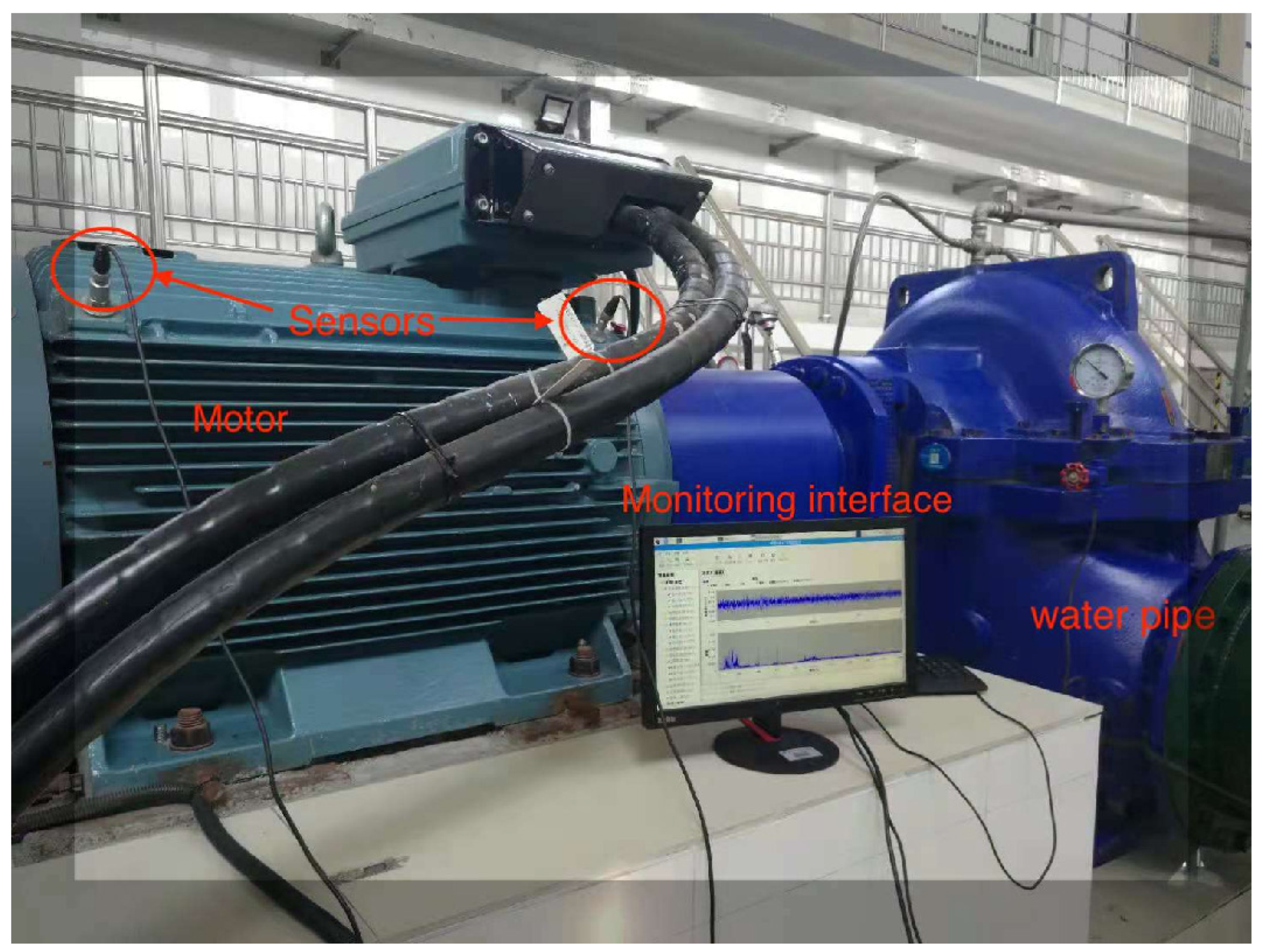
Finally, we deployed the monitoring system we developed to vibration monitoring of water pumps in a water company. At the test site shown in Figure 6, there are seven large-scale pumps, as well as gearboxes and pipes. The vibration acceleration sensor is attached to the pump/motor housing with a strong magnet. The Raspberry Pi embedded system is connected to the DAU via a 5G industrial router. We verified the accuracy of our monitoring system by comparing the measurement results with those of the AR63A, a dedicated instrument used for field testing by the water company. The measurement results show that the performance of our monitoring system is consistent with those of the AR63A. To verify whether the vibration analysis platform works properly over time, the stability of the system needs to be tested. No faults were detected in the tests because the device was operating normally and could not be intentionally damaged to create faults. However, for the noise brought by the external power supply of the DAU, the power harmonic can be for seen from the spectrum. Moreover, the collected vibration signal is usually coupled with heavy noises, such as stemming from sensor imperfections, poor running environment, or background noise, and so on. Besides, the vibration signals are normally non-stationary and nonlinear. What is worse, is that the vibration signal may be too weak to be distinguished from the noise. Therefore, it is still a challenge to extract vibration signals for fault diagnosis under high noise levels and strong harmonic interference.
Several of the above experimental measurements show that the proposed fault prognosis algorithm meets the needs of the water company. We are also well aware that more advanced deep learning-based algorithms, such as those proposed in [26,27], use non-contact vibration images for fault diagnosis and work well under strong noise. The designed analyzer uploads the raw vibration data that the proposed fault prognosis algorithm has assessed to be faulty to a remote server. This provides a sufficient source of data for subsequent deep learning-based algorithms.
5. Conclusions
Modern industrial equipment has improved to a great extent for production efficiency and labor cost, and are moving towards higher precision. High-precision equipment will bring a relatively high abnormality rate. Through experimental tests, the proposed test platform is convenient for users to view the real-time data and graphs. Furthermore, users can also log into the proposed test platform with “VNC viewer” tool software to view real-time monitoring information of the long-running object under test remotely. The test platform is implemented in software, except for the necessary hardware. Therefore, better performance can be obtained by updating the algorithm. By using 5G networks, the raw data of vibration signals are uploaded to the server, which provides a huge amount of data for machine learning and artificial intelligence. The proposed test platform has a wide application value.
The statistical features of vibration signals, such as peak value, peak-to-peak (p2p) value, root-mean-square (RMS), crest factor skewness, kurtosis, spectral kurtosis, impulse factor, shape factor, and clearance factor, are suggested to determine the health state of machinery. However, how to choose appropriate feature parameters to distinguish a healthy state from a faulty state is a key problem. Furthermore, how to differentiate among faulty states is an even more crucial problem. We will intend to work on a solution to these problem with the help of machine learning and artificial intelligence.
Author Contributions
Conceptualization and methodology, K.W.; software Z.-J.X.; writing—original draft preparation, K.W.; writing—review and editing, Z.-J.X. and K.-L.D.; project administration, Y.G.; funding acquisition, Z.-J.X. and Y.G. All authors have read and agreed to the published version of the manuscript.
Funding
This work was funded in part by the Science and Technology Project Funds of Zhejiang Provincial Water Resources Department under Grant no. RC2162, and in part by the National Natural Science Foundation of China under Grant no. 62071212.
Institutional Review Board Statement
Not applicable.
Informed Consent Statement
Not applicable.
Data Availability Statement
Not applicable.
Acknowledgments
The authors thank the anonymous reviewers for their time and efforts spent in evaluating our manuscript and providing constructive comments to improve the manuscript.
Conflicts of Interest
The authors declare no conflict of interest.
References
- Yang, Y.; Zeng, Q.; Yin, G.; Wan, L. Vibration Test of Signal Coal Gangue Particle Directly Impacting the Metal Plate and the Study of Coal Gangue Recognition Based on Vibration Signal and Stacking Integration. IEEE Access 2019, 7, 106784–106805. [Google Scholar] [CrossRef]
- Huang, J.; Chen, G.; Shu, L.; Wang, S.; Zhang, Y. An Experimental Study of Clogging Fault Diagnosis in Heat Exchangers Based on Vibration Signals. IEEE Access 2016, 4, 1800–1809. [Google Scholar] [CrossRef] [Green Version]
- Duan, R.; Wang, F. Fault Diagnosis of On-load Tap-changer in Converter Transformer Based on Time-Frequency Vibration Analysis. IEEE Trans. Ind. Electron. 2016, 63, 3815–3823. [Google Scholar] [CrossRef]
- Bagheri, M.; Zollanvari, A.; Nezhivenko, S. Transformer Fault Condition Prognosis Using Vibration Signals over Cloud Environment. IEEE Access 2018, 6, 9862–9874. [Google Scholar] [CrossRef]
- Chen, S.; Yang, Y.; Dong, X.; Xing, G.; Peng, Z.; Zhang, W. Warped Variational Mode Decomposition with Application to Vibration Signals of Varying-Speed Rotating Machineries. IEEE Trans. Instrum. Meas. 2019, 68, 2755–2767. [Google Scholar] [CrossRef]
- Chen, S.; Yang, Y.; Wei, K.; Dong, X.; Peng, Z.; Zhang, W. Time-Varying Frequency-Modulated Component Extraction Based on Parameterized Demodulation and Singular Value Decomposition. IEEE Trans. Instrum. Meas. 2016, 65, 276–285. [Google Scholar] [CrossRef]
- Hu, Z.; Chen, Z.; Gui, W.; Jiang, B. Adaptive PCA Based Fault Diagnosis Scheme in Imperial Smelting Process. ISA Trans. 2014, 53, 1446–1455. [Google Scholar] [CrossRef] [PubMed]
- Yu, J.; Hu, T.; Liu, H. A New Morphological Filter for Fault Feature Extraction of Vibration Signals. IEEE Access 2019, 7, 53743–53753. [Google Scholar] [CrossRef]
- Chen, S.; Dong, X.; Xiong, Y.; Peng, Z.; Zhang, W. Nonstationary Signal Denoising Using an Envelope-Tracking Filter. IEEE/ASME Trans. Mech. 2018, 23, 2004–2015. [Google Scholar] [CrossRef]
- Yang, Y.; Dong, X.; Peng, Z.; Zhang, W.; Meng, G. Component Extraction for Non-Stationary Multi-Component Signal Using Parameterized De-chirping and Band-Pass Filter. IEEE Signal Process. Lett. 2015, 22, 1373–1377. [Google Scholar] [CrossRef]
- Jenkins, G.; Watts, D. Spectral Analysis and Its Applications, 1st ed.; Holden-Day Press: San Francisco, CA, USA, 1968; pp. 209–257. [Google Scholar]
- Lozano, M.; Fiz, J.; Jane, R. Performance Evaluation of the Hilbert-Huang Transform for Respiratory Sound Analysis and Its Application to Continuous Adventitious Sound Characterization. Signal Process. 2016, 120, 99–116. [Google Scholar] [CrossRef] [Green Version]
- Thirumala, K.; Jain, T.; Umarikar, A. Visualizing Time-Varying Power Quality Indices Using Generalized Empirical Wavelet Transform. Electr. Power Syst. Res. 2017, 143, 99–109. [Google Scholar] [CrossRef]
- Cao, H.; Fan, F.; Zhou, K.; He, Z. Wheel-Bearing Fault Diagnosis of Trains Using Empirical Wavelet Transform. Measurement 2016, 82, 439–449. [Google Scholar] [CrossRef]
- Mey, O.; Neudeck, W.; Schneider, A.; Enge-Rosenblatt, O. Machine Learning-Based Unbalance Detection of a Rotating Shaft Using Vibration Data. In Proceedings of the 2020 25th IEEE International Conference on Emerging Technologies and Factory Automation (ETFA), Vienna, Austria, 8–11 September 2020; pp. 1610–1617. [Google Scholar] [CrossRef]
- Sun, C.; Yin, H.; Li, Y.; Chai, Y. A Novel Rolling Bearing Vibration Impulsive Signals Detection Approach Based on Dictionary Learning. IEEE/CAA J. Autom. Sin. 2021, 8, 1188–1198. [Google Scholar] [CrossRef]
- Umbrajkaar, A.; Krishnamoorthy, A.; Dhumale, R. Vibration Analysis of Shaft Misalignment Using Machine Learning Approach under Variable Load Conditions. Shock. Vib. 2020, 2020, 1650270. [Google Scholar] [CrossRef]
- Öcalan, G.; Türkoğlu, İ. Fault Diagnosis of Rotating Machines Using Raw Vibration Signals and Deep Learning. In Proceedings of the 2021 Innovations in Intelligent Systems and Applications Conference (ASYU), Elaziq, Turkey, 6–8 October 2021; pp. 1–7. [Google Scholar] [CrossRef]
- Irgat, E.; Çinar, E.; Ünsal, A. The detection of bearing faults for induction motors by using vibration signals and machine learning. In Proceedings of the 2021 IEEE 13th International Symposium on Diagnostics for Electrical Machines, Power Electronics and Drives (SDEMPED), Dallas, TX, USA, 22–25 August 2021; pp. 447–453. [Google Scholar] [CrossRef]
- Luo, H.; He, C.; Zhou, J.; Zhang, L. Rolling Bearing Sub-Health Recognition via Extreme Learning Machine Based on Deep Belief Network Optimized by Improved Fireworks. IEEE Access 2021, 9, 42013–42026. [Google Scholar] [CrossRef]
- Shomaki, A.; Alkishriwo, O. Bearing Fault Diagnoses Using Wavelet Transform and Discrete Fourier Transform with Deep Learning. In Proceedings of the 2021 IEEE 1st International Maghreb Meeting of the Conference on Sciences and Techniques of Automatic Control and Computer Engineering MI-STA, Tripoli, Libya, 25–27 May 2021; pp. 744–747. [Google Scholar] [CrossRef]
- Hosameldin, A.; Asoke, K. Condition Monitoring with Vibration Signals: Compressive Sampling and Learning Algorithms for Rotating Machines, 1st ed.; Wiley-IEEE Press: Hoboken, NJ, USA, 2019; pp. 117–128. [Google Scholar]
- Goswami, J.; Hoefel, A. Algorithms for Estimating Instantaneous Frequency. Signal Process. 2014, 84, 1423–1427. [Google Scholar] [CrossRef]
- Frigo, M.; Johnson, S. Fastest Fourier Transform in the West. Available online: http://www.fftw.org (accessed on 10 March 2022).
- Xu, L.; Fang, L.; Lin, C.; Guo, D.; Qi, Z.; Huo, R. Design of Distance Measuring System Based on MEMS Accelerometer. J. Electr. Eng. Technol. 2019, 14, 1675–1682. [Google Scholar] [CrossRef]
- Fan, H.; Xue, C.; Zhang, X.; Cao, X.; Gao, S.; Shao, S. Vibration Images-Driven Fault Diagnosis Based on CNN and Transfer Learning of Rolling Bearing under Strong Noise. Shock. Vib. 2021, 2021, 6616592. [Google Scholar] [CrossRef]
- Anurag, C.; Tauheed, M.; Shahab, F. Convolutional Neural Network Based Bearing Fault Diagnosis of Rotating Machine Using Thermal Images. Measurement 2021, 176, 109196. [Google Scholar] [CrossRef]
Figure 1.
Block diagram of the test platform.

Figure 2.
Software flow of the vibration analysis.

Figure 3.
Real-time monitoring GUI for Raspberry Pi-based vibration test platform.

Figure 4.
The side bands in simulated gearbox vibration signals by using cepstrum analysis.

Figure 5.
Measurement settings interface.

Figure 6.
Water pump room of a water supply company with seven large-scale pumps, including gearboxes and water pipes.
Figure 6.
Water pump room of a water supply company with seven large-scale pumps, including gearboxes and water pipes.


Table 1.
Dynamic performance of YXS-8908 vibration acceleration sensor.
| Measurement range (Peak) | ±5 g (1 g ≈ 9.8 m/s) |
| Sensitivity (25 C) ± 5% | 100 mV/g (160 Hz) |
| Amplitude nonlinearity | ±1% |
| Frequency response | 1∼10,000 Hz (3 dB) |
| Transverse sensitivity ratio | ≤5% |
Publisher’s Note: MDPI stays neutral with regard to jurisdictional claims in published maps and institutional affiliations. |
© 2022 by the authors. Licensee MDPI, Basel, Switzerland. This article is an open access article distributed under the terms and conditions of the Creative Commons Attribution (CC BY) license (https://creativecommons.org/licenses/by/4.0/).
Share and Cite
MDPI and ACS Style
Wang, K.; Xu, Z.-J.; Gong, Y.; Du, K.-L. Mechanical Fault Prognosis through Spectral Analysis of Vibration Signals. Algorithms 2022, 15, 94. https://0-doi-org.brum.beds.ac.uk/10.3390/a15030094
AMA Style
Wang K, Xu Z-J, Gong Y, Du K-L. Mechanical Fault Prognosis through Spectral Analysis of Vibration Signals. Algorithms. 2022; 15(3):94. https://0-doi-org.brum.beds.ac.uk/10.3390/a15030094
Chicago/Turabian StyleWang, Kang, Zhi-Jiang Xu, Yi Gong, and Ke-Lin Du. 2022. "Mechanical Fault Prognosis through Spectral Analysis of Vibration Signals" Algorithms 15, no. 3: 94. https://0-doi-org.brum.beds.ac.uk/10.3390/a15030094
Note that from the first issue of 2016, this journal uses article numbers instead of page numbers. See further details here.