Influence of Swept Blades on Low-Order Acoustic Prediction for Axial Fans

Abstract

The low-speed fans used for automotive engine cooling contribute to a significant part of the global noise emitted by the vehicle. A low-order sound-prediction methodology is developed considering the blade sweep-angle effect on the acoustic predictions of the turbulence-impingement and the trailing-edge noise-generating mechanisms. We modeled these through the application of a semianalytical method based on Amiet’s airfoil theory, appropriately adapted via a strip-theory approach accounting for rotation and modified to include the blades forward curvature. Sweep was already shown in the literature to reduce the noise emitted by isolated airfoils, but its effect on rotating machines was not yet well understood. In this study, we show that the effect of the sweep-angle is to globally reduce the emitted noise by the fan and to change the sound distribution of the sources along the blade span. Thus, the sweep-angle must be considered not only because it yields a better comparison with experimental results but also because wrong conclusions on the dominating noise-generating mechanisms can be drawn when this effect is not taken into account. The investigation is finally complemented by a sensitivity analysis focusing on some of the key parameters characterizing the acoustic prediction.

1. Introduction

Several industrial fields, such as the aeronautical, automotive, wind-turbines and the ventilation of buildings sectors are concerned with the acoustic radiation of rotational machinery [1,2,3,4]. Blade sweep is considered as a classical technique in order to mitigate the far-field emissions as well as to enhance the aerodynamic efficiency [5]. In the automotive field, low-speed cooling fans [6] are used to cool down the engine of the car by extracting hot air out of heat exchangers [7]. Several noise-generating mechanisms of tonal and broadband nature occur in this application [8], where backward-swept and forward-swept propellers are often employed [9]. Among the most influencing sound source mechanisms, one distinguishes the turbulence-interaction or leading-edge one and the trailing-edge or self-noise mechanism [10]. These are analogously studied in turbofans propellers as reported in [11]. Following the semianalytical works carried out in [12,13,14,15] for the previous two broadband mechanisms, the aim of this study is to implement semianalytical methods, based on Amiet’s airfoil noise theory [16,17], able to take into account the effect of having swept leading- and trailing-edges. Although these methodologies were already proven to accurately model the noise emitted by static swept airfoils, to the authors’ knowledge, no application to low-speed rotating blades has been carried out so far including sweep, in order to predict the overall broadband emitted sound. Nevertheless, the work of Roger et al. [14] aimed at modeling tonal noise emissions by Contra-Rotating Open Rotors (CRORs) and was instrumental in deriving the set of equations hereafter adapted to model the leading-edge noise for low-speed cooling fans.

In a recent work [18], the authors implemented a low-order prediction methodology that was only including the trailing-edge noise modeling neglecting the acoustic influence of blades with varying sweep angle. The following study is intended to be a continuation of this work and thus, the same experimental measurements and CFD simulation are considered hereafter. In this work, the leading-edge noise prediction has been included in the low-order acoustic methodology and both the trailing- and leading-edge noise formulations are now considering the presence of a radius-dependent sweep angle. The purpose of this work is to highlight the importance of modeling the sweep effects but also to carry out a sensitivity study in order to understand better the influence of some of the several parameters characterizing the application of Amiet’s theory for trailing- and leading-edge noise prediction. In order to model the former, several semiempirical wall-pressure models have been proposed in literature [19], but a few studies were carried out to assess their validity for rotating blades sound emissions, especially in automotive low-speed fans [12,18]. Moreover, for these applications, the Corcos’ model [20] is generally employed [21] to estimate the spanwise integral length scale $l_y$. Nevertheless, as pointed out in [13], having skewed blade edges may lead to a different redistribution of the spectral energy over the two wavenumbers, ultimately yielding a wrong estimation of $l_y$. To overcome this problem, the Generalized Corcos’ Model proposed by Caiazzo et al. [22] is implemented following the work of Grasso et al. [13], and several combinations of the Butterworth-filter order coefficients are examined in the results section. Regarding the turbulent impingement noise, to the authors’ knowledge, no guidelines are present in literature about the upstream location at which one has to collect the CFD information to feed Amiet’s airfoil theory: a certain location is chosen in this work by examining the overall emitted sound as a function of the leading-edge upstream distance.

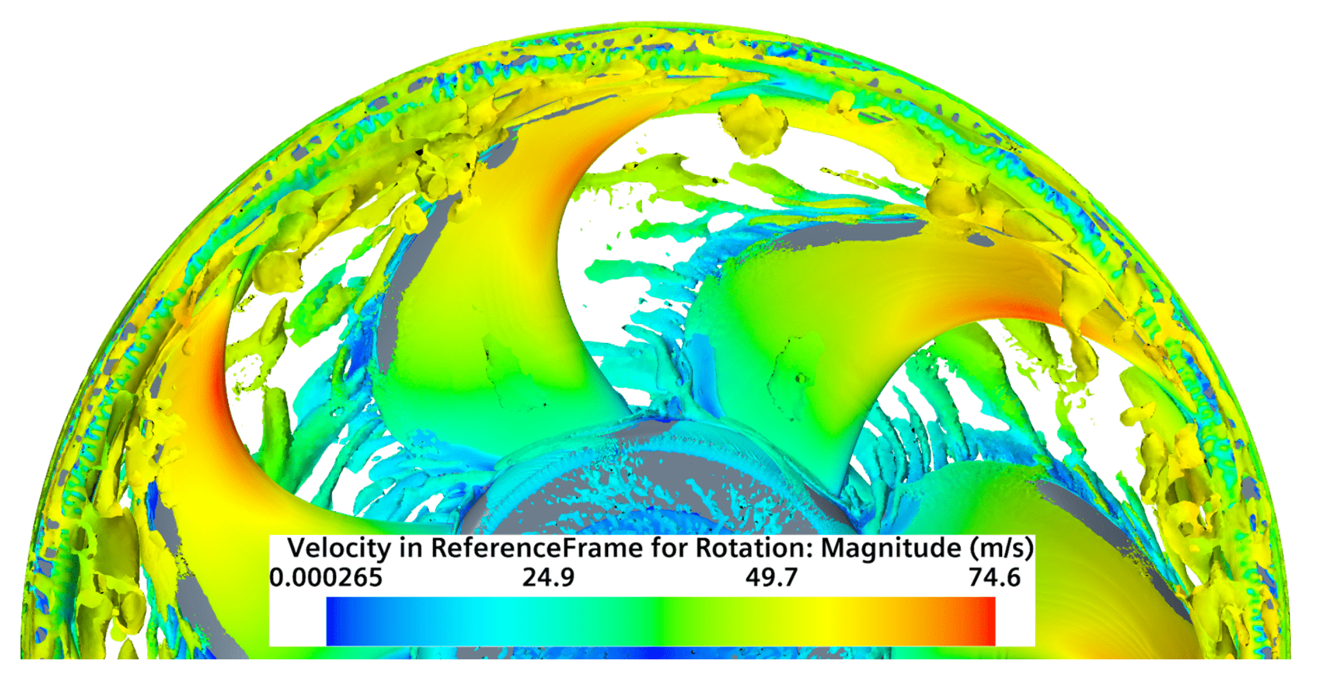
The limitations of the methodology proposed in the following work mainly consist in the lack of modeling of sound-source mechanisms governed by large vortical structures that are particularly dominant sources in the low-frequency range and that require higher-order CFD methods to be simulated. For these systems, in fact, the secondary flow passing through the gap between the ring and the shroud can reach $6\%$ of the nominal flow rate [7]. As shown by an unsteady detached-eddy computation of the same fan in Figure 1, the Q-criterion technique depicts complex vortical structures developing all around the rotating ring. This suggests the presence of large coherent eddies that are not captured by steady calculations and that are probably responsible for the typical subharmonic humps characterizing the low-frequency spectrum, as discussed in [23,24]. Other secondary structures can be localized at the blade cusp regions near the hub, as showed in [25]. This work remains focused on the turbulence impingement and self-noise which are contributing to most of the broadband content from the middle to high frequencies. The paper is organized as follows: Section 2 presents the experimental setup where acoustic measures were acquired at the von Karman Institute for Fluid Dynamics, as described in [18], as well as the installed automotive fan with its geometry and characteristics; in Section 3 the numerical simulation is reported with a focus on the extraction parameters needed to feed the acoustic methodology; the latter is detailed in Section 4, describing the strip-theory approach followed by the inclusion of the sweep angle in Amiet’s airfoil theory; finally, Section 5 illustrates the far-field acoustic results, involving a parametric study and highlighting the importance of taking into account the sweep-angle effects.

2. Experimental Setup

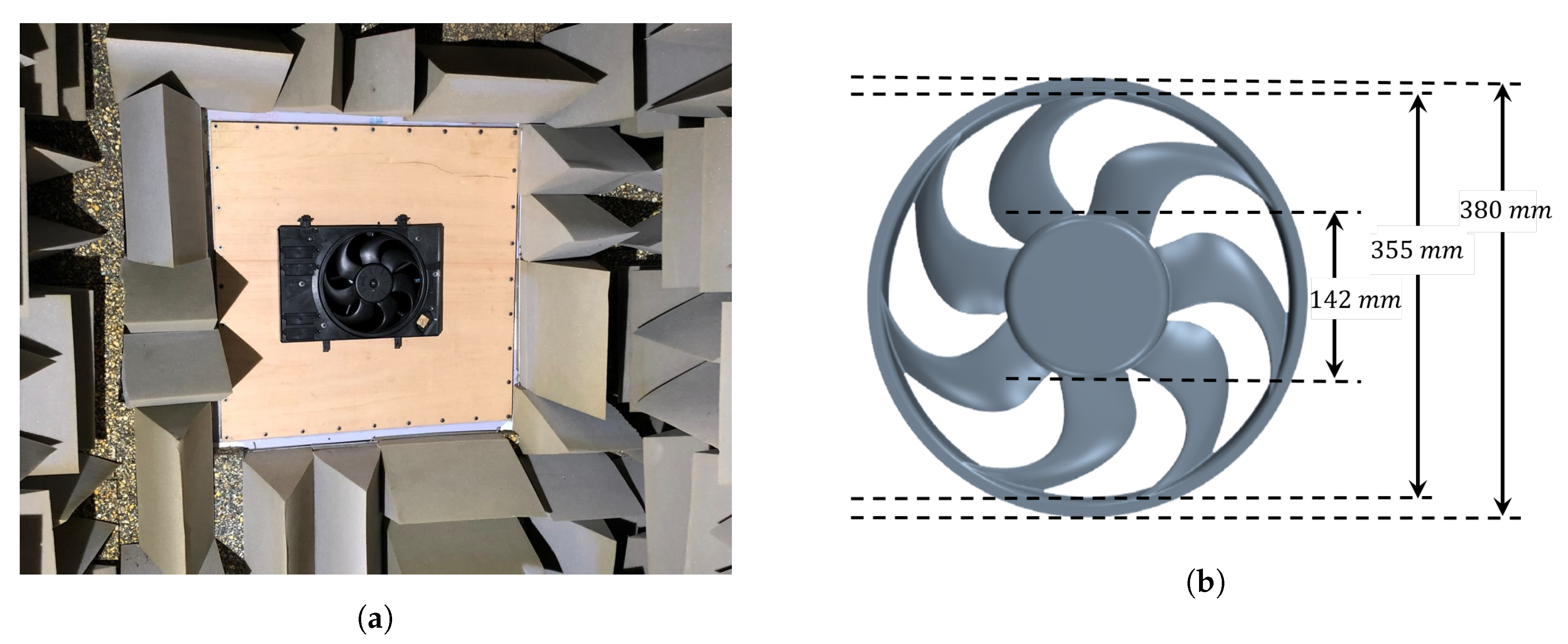
The experimental campaign and the CFD study carried out at the von Karman Institute for Fluid Dynamics in [18] are used as a base to investigate the sweep-angle effect inclusion within the proposed analytical formulation and in order to compare it with a real application. The cooling module has been mounted in the ALCOVES anechoic chamber in an open-rotor configuration, as depicted in Figure 2a, and its far-field sound spectrum has been measured for the fan nominal working condition at one-meter distance, aligned with the center of the fan. The laboratory has been designed by Bilka et al. [26] to have low turbulence level at the inlet and an acoustic cut-off frequency of 150 $\mathrm{Hz}$.

The chosen fan has 7-unequally-spaced blades that are forward skewed, with high sweep-angle values particularly at the tip of the blades. The sweep angle, defined as the angle between the radius and the local tangent to the blade curvature, at the leading edge, reaches very high values of about 70 degrees at the tip of the blade. A slower increase of up to about 50 degrees is attained by the trailing-edge curvature at the blade tip.

3. Numerical Simulation and RANS Extraction Procedure

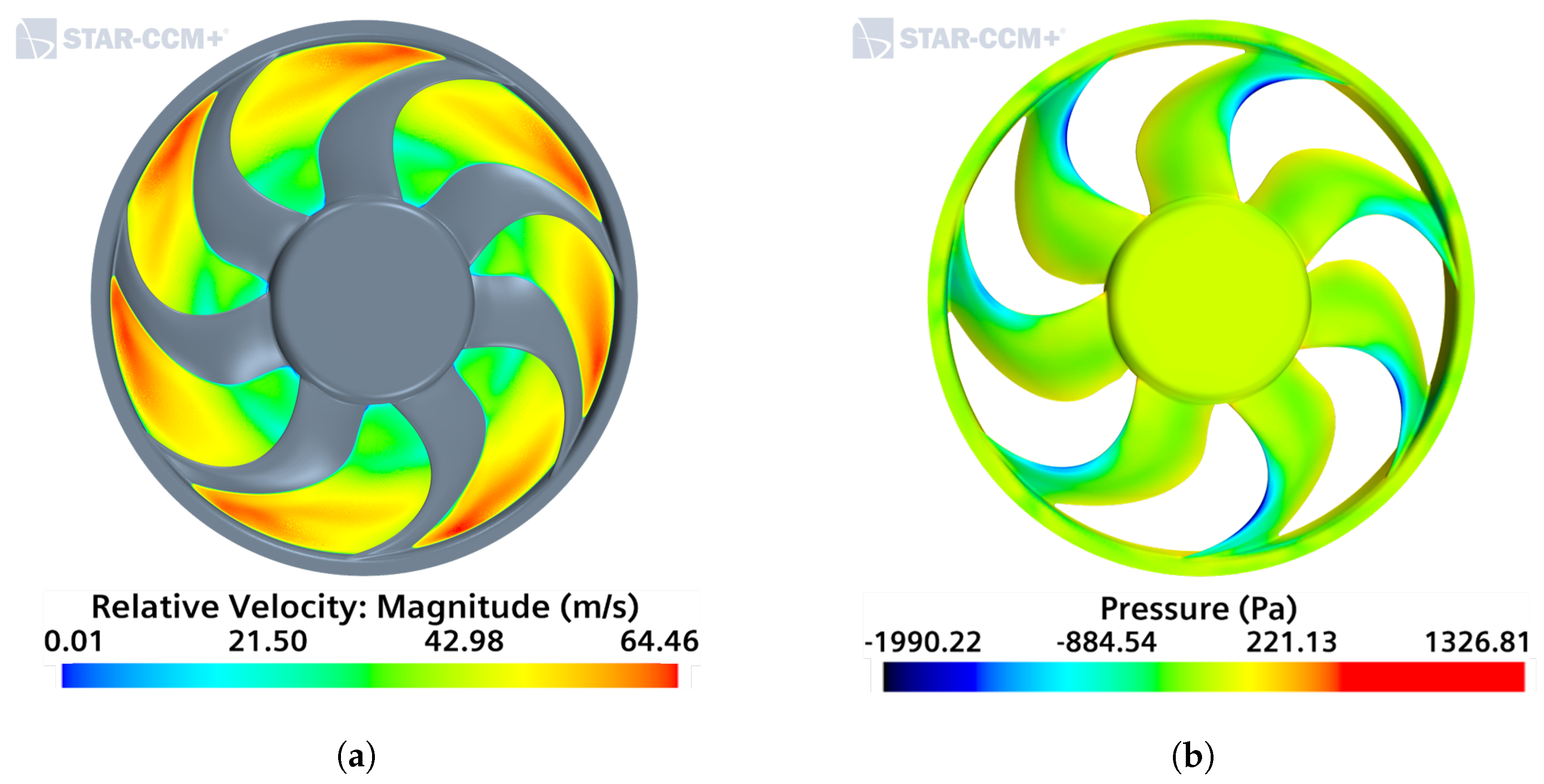
A 3D modeling of the fan installed in ALCOVES anechoic chamber has been employed and is shown in Figure 2b. Steady Reynolds-Averaged Navier-Stokes simulations (RANS), coupled with $k_t-{\omega }_t$ SST turbulence model [27] are chosen as a fair compromise between the computational cost and the simulation accuracy in describing the near-field flow characteristics. The seven blades present similar aerodynamics properties, where at the tip the highest values of mean velocities are observed in Figure 3a. Moreover, the pressure load on the fan suction side presents similar distribution over the blades, with higher values at their leading-edge tip, as Figure 3b shows. For these reasons, only one blade has been used for the following acoustics results. This assumption could not be done in advance because the blades are not equally spaced. The mesh is composed of about 25 million polyhedral cells with a very fine refinement around the blades, in order to capture the viscous sublayer features by keeping a $y^{+}\approx 1$ everywhere, whereas mass-inlet and pressure-outlet boundary conditions are defined. A moving-reference frame approach with a rotational velocity of 3400 rpm is defined near the fan. More details on the mesh geometry and on the inlet and outlet boundary conditions are given in [18]. Furthermore, a similar simulation strategy, despite the use of an unsteady approach in that case, can be found in [7] where the analyzed forward-skewed fan is a slightly bigger sample of the same rotor family produced by Valeo.

3.1. Inlet Turbulence

In order to feed the leading-edge noise formulation with the RANS-based parameters (turbulence kinetic energy $k_t$, specific rate of dissipation ${\omega }_t$, and mean relative or entrainment velocity $U_0$), point-wise locations upstream of the blade leading-edge line are defined. Two quantities are related to the turbulent $k_t-{\omega }_t$ STT model parameters, illustrated by defining the radial normalized distance $y/L_B$: the turbulent length scale ${\Lambda }_f$ in Figure 4a and the mean square of the velocity fluctuations $\overline{u^2}$, in Figure 4b.

The former influences the slopes and the roll-off frequency location of the turbulent velocity fluctuations spectrum and is defined as:

$${\Lambda }_f=\frac{B_t{k}_t^{1/2}}{{\omega }_t{C}_{\mu }},$$

(1)

with the empirical constant $B_t=0.4$ given in [28] and $C_{\mu }=0.09$ given in [29]. The amplitude of the spectrum of the turbulent velocity fluctuations (see Section 4.2) is mostly affected by $\overline{u^2}$, directly linked to the turbulent kinetic energy as $\overline{u^2}=\frac{2}{3}{k}_t$. In Figure 4a, it is worth noticing that $\overline{u^2}$ reaches a peak in the range $0.15<y/L_B<0.45$ and then it starts to grow again while approaching the tip of the blade. Similar trends have been found in the RMS velocity components of Figure 10 in [25].

3.2. Boundary-Layer Parameters

The steady-RANS simulation provides a statistically converged solution of the velocity field around the fan blades. We are interested in extracting the trailing-edge velocity boundary layers at several spanwise locations in order to implement the strip-theory approach presented in Section 4. By so doing, it is possible to estimate the boundary-layer parameters to model the trailing-edge wall-pressure spectra. For automotive forward-skewed fans as the sample considered in this work, it is not trivial to define an external boundary-layer velocity $U_e$ because secondary flows, especially at the blade tip and hub regions as well as flow separation zones can easily occur. For three spanwise locations illustrated in Figure 5a, the boundary-layer thickness $\delta$ (shown with red dots) has been defined at the location normal to the blade where $\delta =\delta (U_e)$.

The external velocity has been calculated with two methods, the first one consisting of using the boundary-layer maximum velocity, such that $U_e=0.99U_{max}$. To ensure the validity of the previous assumption, the total pressure boundary-layer profiles are calculated so that $U_e$ is found at the location where the total pressure reaches its maximum, similarly to what has been done in [12]. The previous methods lead to the same external velocity values and thus, the latter has been used in the following investigations. We define the displacement and momentum thickness, respectively as ${\delta }^{*}$ and $\theta$, by integrating the velocity over the boundary-layer thickness length:

$${\delta }^{*}={\int }_0^{\delta }\left(1-\frac{U(y)}{U_e}\right)dy,$$

(2)

$$\theta ={\int }_0^{\delta }\frac{U(y)}{U_e}\left(1-\frac{U(y)}{U_e}\right)dy.$$

(3)

The pressure coefficient $C_p$ at three spanwise locations is plotted as a function of the chord (where $x_c/c=0$ at the leading-edge point) and is defined as:

$$C_p=\frac{p-p_{\infty }}{\frac{1}{2}{\rho }_{\infty }{U}_0^2},$$

(4)

with $U_0=r\Omega$ as the local entrainment velocity, whereas $p_{\infty }$ and ${\rho }_{\infty }$ are the laboratory pressure and air density, respectively. One can notice that we are in the presence of adverse pressure gradients on the blade suction side at the trailing-edge location regions ($x_c/c>0.8$) and therefore semiempirical wall-pressure models that take them into account are implemented and discussed in Section 4.5.

4. Theoretical Background on Noise Prediction Methodology

An extension of Amiet’s theory to rotating blades, initially developed by Schlinker and Amiet [30] and subsequently by Rozenberg et al. [15], is firstly proposed in order to take into account leading-edge and trailing-edge noise mechanisms. Following the work of Sanjose and Moreau [12], the two sound-mechanism models present consistent similarities but will be treated separately when implementing Amiet’s airfoil theory with or without taking into account the sweep-angle effect.

4.1. Noise Emitted by Rotating Blades

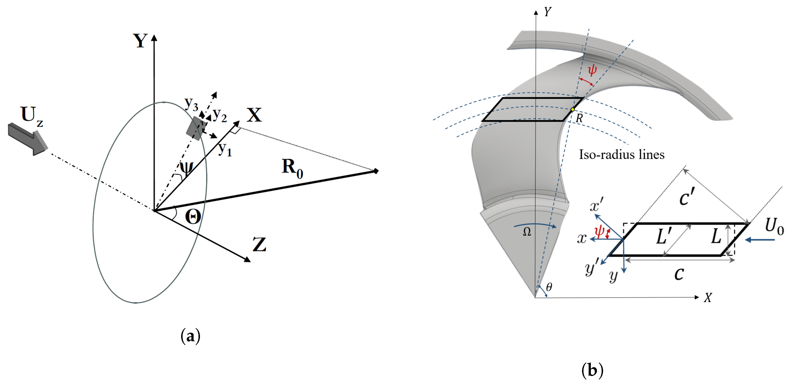
To deal with spanwise-varying conditions, the fan blade is subdivided into strips (or segments) through isoradial cuts such that each strip encounters its own flow condition. The overall radiated fan noise is calculated as the summation of the sound individually emitted by each strip to which the single-airfoil theory is applied, assuming that the circular motion can be approximated by an equivalent local translation. The relative motion between the listener and the source is afterwards considered by including a Doppler frequency-shift factor and taking into account all the azimuthal blade locations as shown in Figure 6a and expressed by Equation (5).

For a given listener angular frequency $\omega$, the fan radiated noise is calculated as:

$$S_{pp}(\mathbf{x},\omega )=\frac{B}{2\pi }{\int }_0^{2\pi }{\left(\frac{{\omega }_e(\Psi )}{\omega }\right)}^2{S}_{pp}^{\Psi }\left(\mathbf{y},{\omega }_e\right)d\Psi ,$$

(5)

where $\mathbf{x}$ is the vectorial listener’s position, whereas $\mathbf{y}$ is the source location; B represents the blades number, ${\omega }_e(\Psi )$ is the source emitted frequency for a certain azimuthal position expressed by the angle $\Psi =\Omega t$, as depicted in Figure 6a. The Doppler factor has to be squared as proven by Sinayoko et al. [31] and for low-Mach number is given by the relation:

$$\frac{{\omega }_e(\Psi )}{\omega }=1+M_{r}sin\Psi sin\Theta ,$$

(6)

in which $M_r$ is the Mach number of the source relative to the fluid. The term $S_{pp}^{\Psi }(\mathbf{y},{\omega }_e)$ of Equation (6) is obtained from the single-airfoil theory as the sum of the trailing-edge and leading-edge noise contributions such that $S_{pp}^{\Psi }=S_{pp}^{TE}+S_{pp}^{LE}$, discussed in the next paragraphs.

4.2. Leading-Edge Noise Formulation

Based on the classical Amiet’s analytical gust-airfoil interaction noise model [16], Roger et al. in [14] extended the formulation to account for swept blades in order to predict tonal noise emitted by CRORs. In the following work, these developments are used to predict broadband sound sources as carried out for an isolated airfoil in the work of Giez et al. [32]. The sweep angle is defined as the angle between the fan radius line and the line locally tangent to the edge of the blade, as depicted in Figure 6b. A local reference frame $(x,y,z)$ is defined, with the x axis parallel to the flow direction $U_0=\Omega R$ (with the fan angular rotation $\Omega$), the z axis perpendicular to the blade-strip plane and the y axis orthogonal to the previous two, pointing at the center of rotation. A second local reference frame $(x^{\prime },y^{\prime },z)$ is obtained with a clockwise rotation around the z axis by the sweep angle $\psi$; the $y^{\prime }$ axis is now laying on the leading edge of the blade segment. We specify that Figure 6b depicts the case where the reference frames are centered on the trailing-edge, valid for the TE noise formulation discussed later. For the LE formulation, the only difference is that the reference frames are located at the center of the strip, as Figure 7 illustrates. The chord c and span L of the blade segment are equivalently indicated in the same figure, as well as the rotated chord $c^{\prime }=ccos(\psi )$, parallel to $x^{\prime }$, and the rotated span $L^{\prime }=L/cos(\psi )$, parallel to $y^{\prime }$. To have further information about the following formulation, the interested reader can refer to [1,14,33]. We define the acoustic wavenumber $k_a=\frac{\omega }{c_0}$ and the observer corrected distance $S_0$ to take into account the convection effects as:

$$S_0^2={\beta }_y^2{X}^2+{\beta }_x^2{Y}^2+{\beta }_0^2{Z}^2,\mathrm{where}{\beta }_{y,x,0}=\sqrt{1-{\left(\frac{U_{y,x,0}}{c_0}\right)}^2},$$

(7)

where $(X,Y,Z)$ must refer to the rotated reference frame $(x^{\prime },y^{\prime },z)$. Equation (7) introduces the velocity component $U_x=\frac{U_0}{cos\psi }$ perpendicular to the swept leading edge and the one parallel to it $U_y=\frac{U_0}{sin\psi }$. The turbulence is assumed to be isotropic, frozen, and expanded into harmonics gusts. We write the power-spectral density (PSD) of the far-field acoustic pressure for a fluid with the speed of sound $c_0$ and the density ${\rho }_0$, with the assumption of large aspect ratio on the full blade span. This not only yields a simpler mathematical expression of the PSD reported in Equation (8), but it is the only one that converges with the number of the strips. This was discussed in the Ph.D. thesis of Rozenberg (see Section 4.4.5 in [34]) and confirmed by Christophe et al. [35]. We write the PSD of the far-field sound as:

$$S_{pp}^{LE}(\mathbf{x},\omega )={\left(\frac{{\rho }_0\omega b^{\prime }Z}{c_0{S}_0^2}\right)}^{2}2\pi U_x\frac{L^{\prime }}{2}{\Phi }_{ww}\left(\overline{K_x^{\prime }},\overline{K_y^{\prime }}\right){\left|{\mathcal{L}}^{LE}\left(X,K_x^{\prime },K_y^{\prime }\right)\right|}^2,$$

(8)

where $b^{\prime }=c^{\prime }/2$ and $K_y^{\prime }$ is the only involved gust, which can be verified to be always supercritical, as stated in [1], and is expressed as [13,32]:

$$K_y^{\prime }=\frac{k_a}{{\beta }_0^2}\left(\frac{{\beta }_x^{2}Y}{S_0}-\frac{U_y}{c_0}\right).$$

(9)

Given the dispersion equation ${\mathbf{U}}_{\mathbf{0}}·\mathbf{K}=U_x{K}_x^{\prime }+U_y{K}_y^{\prime }$, the $x^{\prime }$-wavenumber is defined as:

$$K_x^{\prime }=\frac{\omega -K_y^{\prime }{U}_y}{U_x}.$$

(10)

The mathematically-derived aeroacoustic wavenumber term ${\mathcal{L}}^{LE}$ does not consider the contribution of the trailing-edge back-scattering derived in [21], which is typically much smaller if compared to the main contribution:

$${\mathcal{L}}^{LE}=-\frac{e^{-i{\Theta }_2}}{\pi }\sqrt{\frac{2}{\left(\overline{K_x^{\prime }}+{\beta }_x^2\kappa \right){\Theta }_1}}E\left[2{\Theta }_1\right].$$

(11)

We define the parameter $\kappa$ as:

$${\kappa }^2={\mu }^2-\frac{{\overline{K_y^{\prime }}}^2}{{\beta }_x^2},\mathrm{with}\mu =\frac{\overline{K_x^{\prime }}{U}_x}{c_0{\beta }_x^2},$$

where $\overline{K_x^{\prime }}$ and $\overline{K_y^{\prime }}$ are the dimensionless wavenumbers; $E[-]$ is the Fresnel integral, whereas ${\Theta }_1$ and ${\Theta }_2$ can be can be written [14,32,33]:

$${\Theta }_1=\left(\kappa -M_x^2\overline{K_x^{\prime }}/{\beta }_x^2\right)+b\left\{tan\psi K_y^{\prime }-\frac{k_a}{{\beta }_0^2{S}_0}\left[{\beta }_y^{2}X-S_0\frac{U_x}{c_0}+tan\psi \left({\beta }_x^{2}Y-S_0\frac{U_y}{c_0}\right)\right]\right\},$$

$${\Theta }_2={\Theta }_1+\left(\frac{U_1^2\overline{K_x^{\prime }}}{c_0^2{\beta }_x^2}-\kappa \right)-\pi /4.$$

The von Kármán’s and Liepmann’s spectrum models, assuming homogeneous isotropic turbulence, are used to calculate the two-wavenumber spectrum ${\Phi }_{ww}(K_x^{\prime },K_y^{\prime })$, analogously to what has been done in [12,36]. Starting off from the steady RANS extracted data of Section 3, we can write the von Kármán’s model spectrum as:

$${\Phi }_{ww}^{VK}\left(K_x^{\prime },K_y^{\prime }\right)=\frac{4}{9\pi }\frac{\overline{u^2}}{k_e^2}\frac{{\widehat{K_x^{\prime }}}^2+{\widehat{K_y^{\prime }}}^2}{{\left(1+{\widehat{K_x^{\prime }}}^2+{\widehat{K_y^{\prime }}}^2\right)}^{7/3}},$$

(12)

whereas, using the Liepmann’s model spectrum:

$${\Phi }_{ww}^{LM}\left(K_x^{\prime },K_y^{\prime }\right)=\frac{3\overline{u^2}{\Lambda }_f^4\left({K_x^{\prime }}^2+{K_y^{\prime }}^2\right)}{4\pi {\left(1+{\Lambda }_f^2\left({K_x^{\prime }}^2+{K_y^{\prime }}^2\right)\right)}^{5/2}},$$

(13)

with $\overline{u^2}$ as the mean square of the velocity fluctuations, which is directly related to the RANS scalar turbulent kinetic energy $k_t$ as: $\overline{u^2}=\frac{2}{3}{k}_t$.

The average wavenumber of the energy-containing eddies $k_e$ in Equation (14) is defined as:

$$k_e=\frac{\sqrt{\pi }}{{\Lambda }_f}\frac{\Gamma (5/6)}{\Gamma (1/3)},$$

(14)

where the turbulent length scales ${\Lambda }_f$ has been defined in Equation (1).

4.3. Trailing-Edge Noise Formulation

According to the original derivation by Amiet [17], afterwards extended by Roger and Moreau [21], the inclusion of the sweep-angle effect for the trailing-edge noise modeling, in this work, followed the recent work of Grasso et al. [13]. The PSD of the far-field noise for the large aspect ratio is given as:

$$S_{pp}^{TE}(\mathbf{x},\omega )={\left(\frac{\omega cos\psi b^{\prime }Z}{2\pi c_0{S}_0^2}\right)}^2\pi L^{\prime }{\left|\mathcal{L}\left({\overline{K}}_c^{\prime },{\overline{K}}_y^{\prime }\right)\right|}^2{\Pi }_0\left(\omega ,{\overline{K}}_y^{\prime }\right).$$

(15)

Consistently with the leading-edge formulation in the previous section, the main contribution of the aeroacoustic transfer function is written:

$${\mathcal{L}}^{TE}=-\frac{{\mathrm{e}}^{2\mathrm{i}\mathrm{C}/\cos \psi }}{\mathrm{i}C}\left\{(1+\mathrm{i}){\mathrm{e}}^{-2\mathrm{i}C/\cos \psi }\sqrt{\frac{2B}{cos\psi }}{\mathrm{ES}}^{*}\left[\frac{2(B-C)}{cos\psi }\right]-(1+\mathrm{i}){\mathrm{E}}^{*}\left[\frac{2B}{cos\psi }\right]+1-{\mathrm{e}}^{-2\mathrm{i}C/cos\psi }\right\},$$

(16)

where the mathematical expressions of the functions $E^{*}[-]$ and $ES[-]$, both closely related to the Fresnel integral, are given for instance in [13]. The parameters B and C can be written as:

$$B=\left(\alpha {\overline{K}}_c^{\prime }+\mu \frac{U_x}{c_0}+\kappa \right)cos\psi ,$$

$$C=\alpha {\overline{K}}_x^{\prime }cos\psi +{\overline{K}}_y^{\prime }sin\psi -\frac{\overline{k_a}}{{\beta }_0^2}\left(\frac{{\beta }_y^{2}xcos\psi }{S_0}+\frac{{\beta }_x^{2}ysin\psi }{S_0}-\frac{U_0}{c_0}\right).$$

The $\overline{K_y^{\prime }}$ term is given by Equation (9), whilst the rotated convective wavenumber is shown in Equation (17):

$$K_c^{\prime }=\frac{\omega }{U_{c}cos\psi }-K_y^{\prime }tan\psi ,$$

(17)

assuming the frozen turbulence hypothesis can be applied such that the convective velocity is determined as $U_c=U_0/\alpha$, with $\alpha =1.43$.

In order to compare with far-field experimental results, as described in the original work of Amiet [17], Equations (8) and (15) have to be multiplied by a factor $b_w=2\pi$ needed to convert to a 1 Hz bandwidth. As indicated by [37], there is no need to multiply Equation (15) by 2 to convert to a single-sided frequency spectrum, as done in [21], because all the wall-pressure models hereafter utilized are already single-sided. Nonetheless, Equation (15) is further multiplied by 2 in order to account for the pressure and suction sides. According to [17], this factor of 2 should be used only for cases where two identical boundary layers are encountered on the pressure and suction sides. Even though with control diffusion airfoils the suction side is typically radiating more than the pressure side [12], the latter cannot be neglected in advance in view of the similar boundary-layer thicknesses. Nonetheless, no semiempirical wall-spectrum model has been conceived to account specifically for favorable pressure gradients that we notice on the pressure-side trailing-edge region, as illustrated in Figure 4b. Hence, this 2 factor is used to be conservative about the emitted trailing-edge noise, yielding to a global multiplication factor of $4\pi$.

4.4. Generalized Corcos’ Model

In Amiet’s classical formulation, the separation of frequency and wavenumber variables of the Corcos’ model [20] is assumed in order to write the wall-pressure PSD ${\Pi }_0(\omega ,K_y)$ of Equation (15) as:

$${\Pi }_0\left(\omega ,K_y\right)={\int }_{-\infty }^{+\infty }\Pi \left(k_x,K_y,\omega \right)d{k}_x=\frac{1}{\pi }{\phi }_{pp}(\omega )l_y\left(\omega /U_c,K_y\right),$$

(18)

where the complete frequency-wavenumbers wall-pressure power-spectral density $\Pi (k_x,K_y,\omega )$ is given by:

$$\Pi \left(k_x,k_y,\omega \right)={\phi }_{pp}(\omega )\frac{\frac{1}{\pi {\alpha }_{\omega }}}{1+{\left(\frac{k_x-k_{\omega }}{{\alpha }_{\omega }}\right)}^2}\frac{\frac{1}{\pi {\beta }_{\omega }}}{1+{\left(\frac{k_y}{{\beta }_{\omega }}\right)}^2},$$

(19)

with $k_{\omega }=\omega /U_c$, ${\alpha }_{\omega }={\alpha }_x\omega /U_c$ and ${\beta }_{\omega }={\beta }_y\omega /U_c$. The coefficients ${\alpha }_x=0.1$ and ${\beta }_y=1/1.47$ are chosen within interval suited for smooth rigid walls [22]. The the spanwise correlation length $l_y(\omega /U_c,K_y)$ in Equation (18) is obtained after integrating over $k_x$ as in [21]:

$$l_y(\omega ,K_y)=\frac{k_{\omega }/b_c}{K_y^2+{(k_{\omega }/b_c)}^2},$$

(20)

with $b_c$ as a constant. Even though the mathematical simplicity of Equation (20) is appealing, taking into account a skewed gust may lead to a wrong estimation of the spectral energy distribution on the streamwise and spanwise rotated wavenumbers. To overcome this problem, Grasso et al. [13] implemented the Generalized Corcos’ model firstly developed in [22]. As introduced in the latter work, the Lorentzian functions originally utilized in the Corcos’ model to describe the two spatial correlation lengths, are interpreted as Butterworth filters of order $m=1$ and $n=1$. Thus, in the general case, Equation (19) can be modified as:

$$\Pi \left(k_x,k_y,\omega \right)={\phi }_{pp}(\omega )\frac{\frac{nsin(\pi /2n)}{\pi {\alpha }_{\omega }}}{1+{\left(\frac{k_x-k_{\omega }}{{\alpha }_{\omega }}\right)}^{2n}}\frac{\frac{msin(\pi /2m)}{\pi \beta \omega }}{1+{\left(\frac{k_y}{{\beta }_{\omega }}\right)}^{2m}}$$

(21)

Caiazzo et al. [22] intended this generalization to correct the low-wavenumber behavior that is causing the original Corcos’ model to overestimate the contribution of the subconvective streamwise wavenumber range to a given angular frequency $\omega$. The filter order coefficients m and n can be seen as free parameters to be adjusted in order to better approximate the experimental wall-pressure spectrum. When introducing the rotated streamwise and spanwise wavenumbers, a coupling between the coherence lengths appears:

$$\Pi \left(k_x^{\prime },k_y^{\prime },\omega \right)={\phi }_{pp}(\omega )\frac{\frac{nsin(\pi /2n)}{\pi {\alpha }_{\omega }}}{1+{\left(\frac{k_x^{\prime }cos\psi +k_y^{\prime }sin\psi -k_{\omega }}{{\alpha }_{\omega }}\right)}^{2n}}\frac{\frac{msin(\pi /2m)}{\pi {\beta }_{\omega }}}{1+{\left(\frac{-k_x^{\prime }sin\psi +k_y^{\prime }cos\psi }{{\beta }_{\omega }}\right)}^{2m}}.$$

(22)

Nevertheless, the analytical integration over $k_x^{\prime }$ is still possible, but rather cumbersome, and it was performed by Grasso et al. [13] for a combination set of m and n order coefficients, by using the open access software named Sage Math. The aim was to calculate a different spanwise correlation length $l_y$ for each couple of m and n with the limit case of Equation (19) when $m=1$, $n=1$. These derivations have been implemented in the following methodology in order to clarify their influence on the far-field radiated sound.

4.5. Semiempirical Wall-Pressure Models

As a closure to Equation (15), semiempirical models have been implemented to calculate the frequency-dependent part of the wall-pressure spectrum (WPS) $\varphi (\omega )$. Originally proposed by Lee [19] and based on the work of Goody [38], a universal formulation can be adopted to describe the shape of $\varphi (\omega )$ and expressed as:

$$\frac{{\varphi }_{pp}}{{\varphi }^{*}}=\frac{a{({\omega }^{*})}^b}{{[i{({\omega }^{*})}^c+d]}^e+{[f{R}_T^g{\omega }^{*}]}^h},$$

(23)

where the parameters $a-h$ are set to modify the shape of the spectra according to the chosen model (more details on the effect of each coefficient can be found in [19,39]), the rescaled wall-pressure spectrum and the circular frequency ${\varphi }^{*}$ and ${\omega }^{*}$, respectively; finally, $R_T$ is the time-scale ratio which accounts for Reynolds number effects. Three different models will be considered hereafter, Goody’s model that is suited to zero-pressure gradient profiles, Rozenberg’s model that is tuned to take into account adverse-pressure gradient profiles, and Lee’s model that is based on the previous two and can be applied in both cases.

4.5.1. Goody’s Model

Goody’s model is based on the work of Chase [40] and Howe [41] and it is often taken as a reference model to compare with more recent ones [19]. The overlap region was extended by introducing the time-scale ratio, defined as the ratio of the outer time scale to the inner time scale as:

$$R_T=(\delta /U_e)/(\nu /u_{\tau }^2),$$

(24)

with the kinematic viscosity $\nu$ and the friction velocity $u_{\tau }$. The angular frequency is scaled by ${\omega }^{*}=\delta /U_e$, whereas the wall-pressure spectrum model is scaled by ${\varphi }^{*}={\tau }_w^2\delta /U_e$, with ${\tau }_w$ as the wall-shear stress (directly related to the friction velocity as $u_{\tau }=\sqrt{{\tau }_w/{\rho }_{\infty }}$), which is estimated in the following sections applying the general method proposed by Bradshaw and Ferriss in [42]. The coefficients given in Equation (23) for the Goody’s model are $a=3.0$, $b=2$, $c=0.75$, $d=0.5$, $e=3.7$, $f=1.1$, $g=-0.57$, $h=7.0$, and $i=1.0$.

4.5.2. Rozenberg’s Model

In order to account for adverse pressure gradient flows, Rozenberg et al. [43] developed a model basing it on Goody’s. The frequency is scaled by ${\omega }^{*}={\delta }^{*}/U_e$, whereas the wall-pressure spectrum normalization is defined as ${\varphi }^{*}={\tau }_{max}^2{\delta }^{*}/U_e$, where the boundary-layer maximum wall-shear stress was introduced. Nevertheless, in this work ${\tau }_w$ has been employed always, as suggested by Lee [19]. Other three parameters are determined to characterize the effect of the adverse pressure gradient: Zagarola-Smits’ parameter ${\Delta }_{*}=\delta /{\delta }^{*}$ [44], Causer’s equilibrium parameter [45] ${\beta }_c=\left(\theta /{\tau }_w\right)(dp/dx)$, and Coles’ wake parameter [46] $\Pi$. The latter is estimated using the empirical formula given by Durbin and Reif in [47], $\Pi =0.8{({\beta }_c+0.5)}^{3/4}$. The other parameters in Section 4.5 are defined as:

• $a=[2.82{\Delta }_{*}^2{\left(6.13{\Delta }_{*}^{-0.75}+d\right)}^e]\left[4.2\left(\Pi /{\Delta }_{*}\right)+1\right]$,
• $b=2.0$,
• $c=0.75$,
• $d=4.76{\left(1.4/{\Delta }_{*}\right)}^{0.75}[0.375e-1]$,
• $e=3.7+1.5{\beta }_c$,
• $f=8.8$,
• $g=-0.57$,
• $h=min\left(3,19/\sqrt{R_T}\right)+7$,
• $i=4.76$.

One may notice that unlike Goody’s model, here the parameters have to be determined as functions of the pressure gradient $dp/dx$, which is directly provided by the RANS computation at the blade wall and it is rotated to follow the isoradial curvature of the blade suction side.

4.5.3. Lee’s Model

Lee [19] recently proposed a model to extend the validity of Rozenberg’s model to low and high pressure gradient flows, as well as to higher ${\beta }_c$ values, for extensive applications. Most of the parameters used for Rozenberg’s model are kept the same with some exceptions discussed hereafter. First, the spectrum is scaled by the wall-shear stress ${\tau }_w$, rather then using the maximum shear stress ${\tau }_{max}$ over the boundary-layer length. To correct the higher amplitudes for low and middle frequencies predicted by Rozenberg’s model in low-pressure gradient flows, the parameter d is modified as $d=max(1.0,1.5d)$ if ${\beta }_c<0.5$. The parameter a is adjusted as $a=max(1,(0.25{\beta }_c-0.52)a)$. To compensate for the rapid decay rate encountered in Rozenberg’s model for zero and low-pressure gradient flows, the parameter h is modified as follows:

$$h=min\left(5.35,0.139+3.1043{\beta }_c,19/\sqrt{R_T}\right)+7,$$

(25)

whereas the following expression has to be used if $h=12.35$:

$$h=min\left(3,19/\sqrt{R_T}\right)+7.$$

(26)

5. Acoustic Far-Field Results

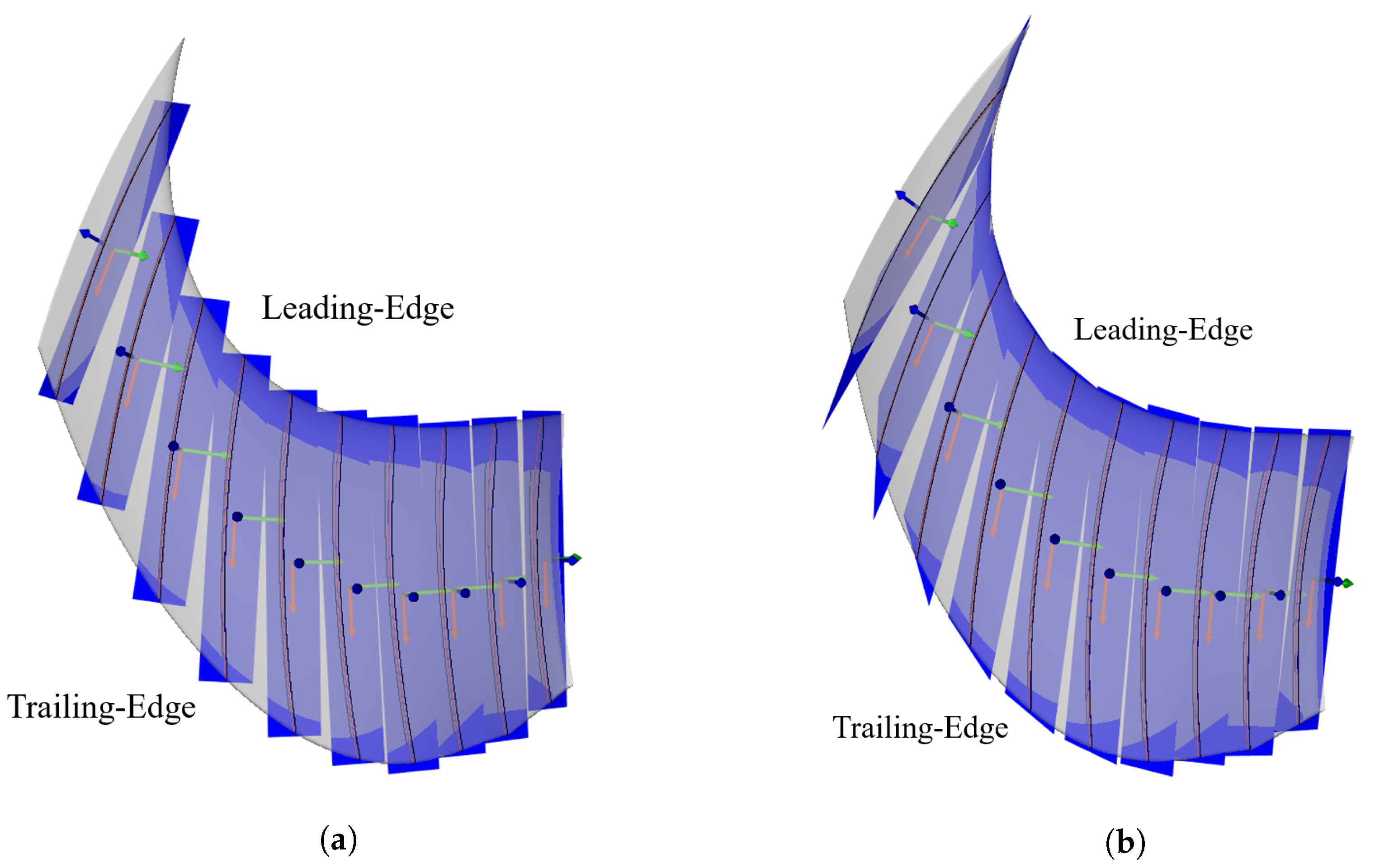
The implementation of the single-airfoil Amiet’s analytical formulations including the sweep-angle effect has been compared and validated with the work of Giez et al. [32] for the LE noise case, and with the work of Grasso et al. [13] for the TE noise case. The strip-theory approach is illustrated in Figure 7a for the LE noise case, where 10 blade strips have been generated together with their local reference frames at the center of the segments performing equidistant cuts along the radius line. An improvement taking into account the sweep angle is shown in Figure 7b, where the leading-edges of the blade planes are now locally parallel to the forward-skewed curvature of the blade.

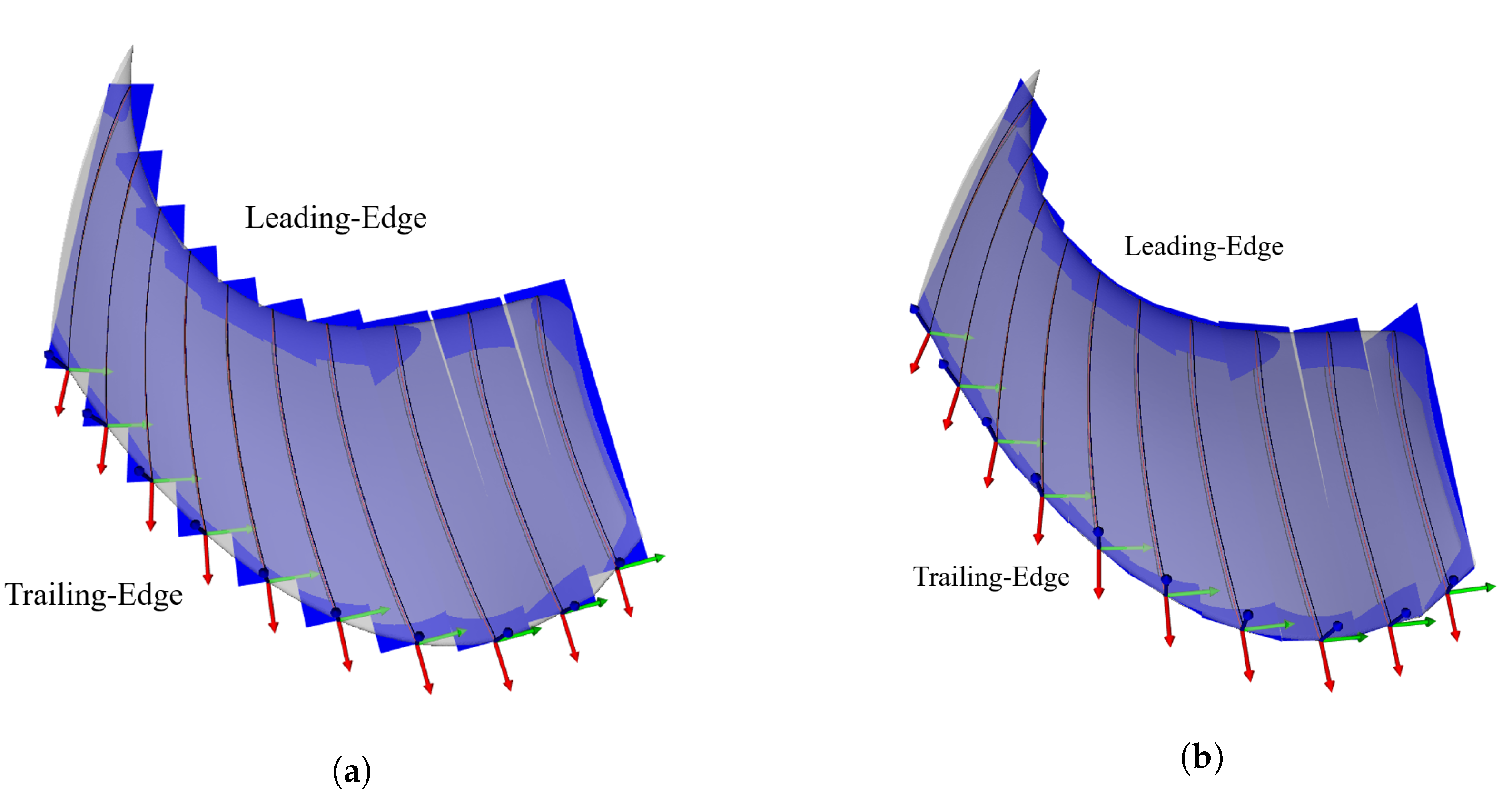
A similar approach has been implemented to carry out the blade segments for the TE formulation as shown in Figure 8. Nevertheless, for this specific case, the blade segments are obtained by subdividing the TE line into equidistant cuts. In fact, it was observed that when the blade is divided into evenly distributed segments over the radius, a systematic underestimation of about 2 dB in the far-field noise is appearing due to the fact that the strips would have a too short span. On the contrary, one can notice in Figure 8b that the trailing-edge line is completely covered using this distribution of the isoradial strips.

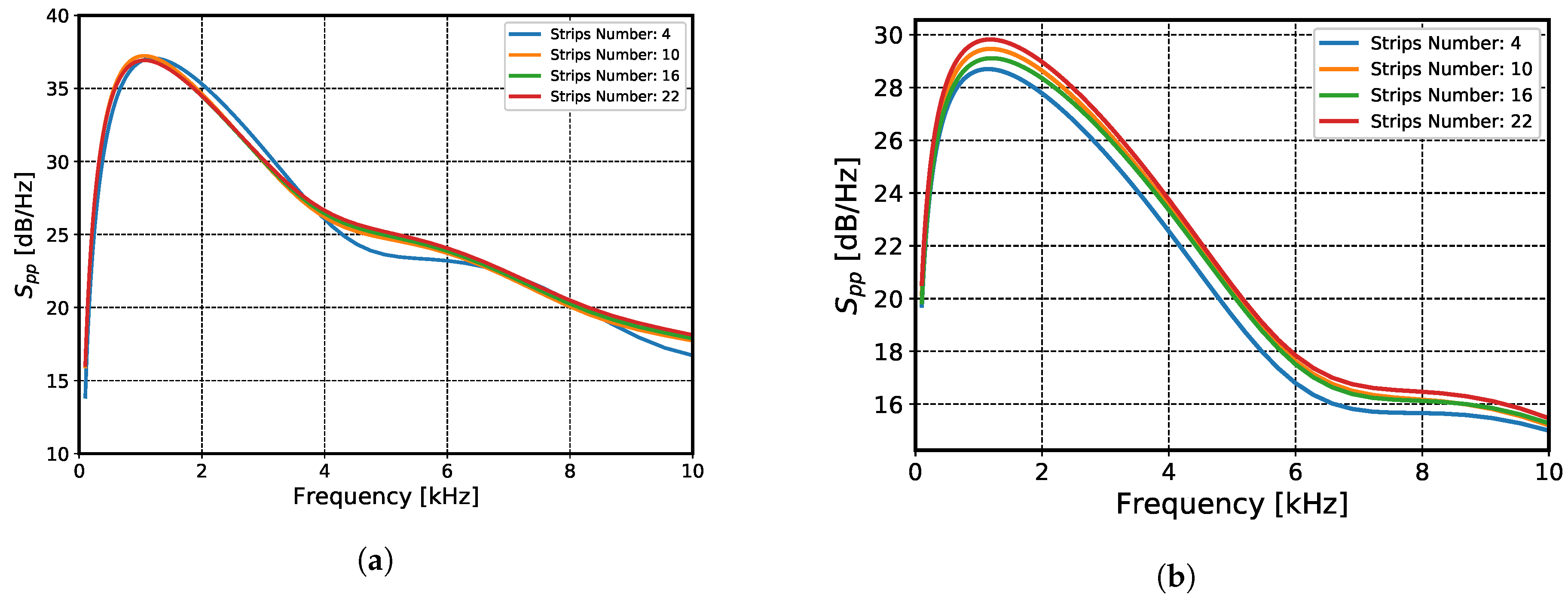
A convergence study was carried out in order to establish the minimum number of strips to acceptably discretize the noise emissions along the blade span. For both sound mechanisms, the blade is finally cut in 16 strips: this value is kept throughout the study. While for the LE case, illustrated in Figure 9a, the convergence is quite fast, for the TE case in Figure 9b small differences up to about 1 dB are depicted between the 16 and 22 strips cases. This is due to the 3D discretization of the blade as well as to the distribution of the strips over the most emitting areas.

5.1. Noise Distribution over the Strips

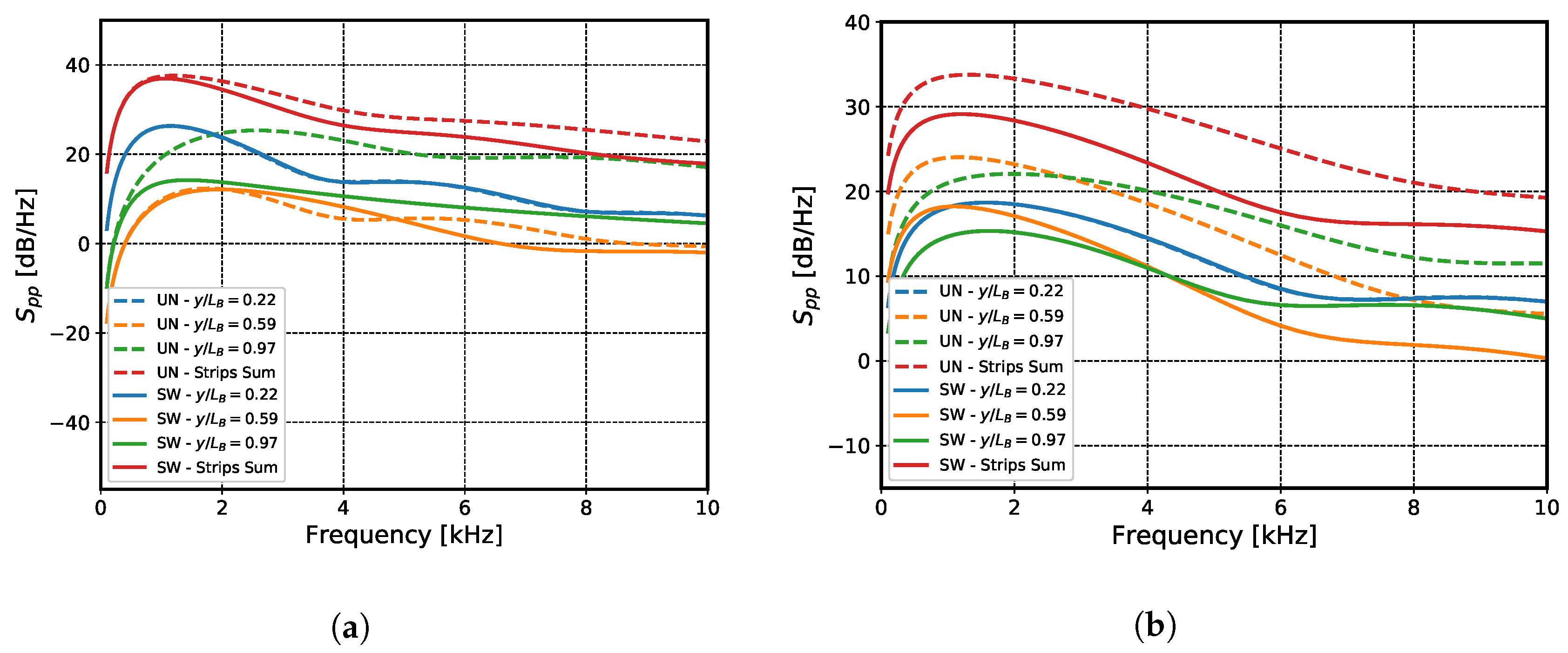
For the two noise mechanisms, the unswept classical Amiet’s formulations [16,17] are retrieved as a limit case where $\psi =0$. In Figure 10, the LE and TE noise methodologies are compared with respect to the unswept Amiet’s formulation. Three strips are reported with a respective distance from the hub of $y/L_B$. In Figure 10, one can generally notice that closer to the tip, the far-field sound predicted by the unswept approach is higher, due to the radial linear increase of the relative velocity. The effect of the sweep is to reduce, mainly in amplitude, the PSD of each strip. We mention that at $y/L_B=0.22$, the local blade sweep is near 0, and therefore the unswept (UN) and swept (SW) formulations give very close results.

For the LE case, depicted in Figure 10a, the unswept formulation shows higher PSD values nearer the tip and beyond 1.9 kHz. Nevertheless, for the swept formulation, the strip at $y/L_B=0.22$ is seen to be louder than the one at $y/L_B=0.59$ throughout all frequencies. For low to middle frequencies, this can be explained by the high values of $\overline{u^2}$, which are found in the range $0.15<y/L_B<0.45$, as depicted in Figure 4a. In fact, the mean square of the velocity fluctuations is directly linked to the turbulent kinetic energy content found in the RANS simulation and depicted in Figure 11a. This increase of $k_t$ has been found in other studies with similar fans, as Figure 9 in [25] illustrates. Particularly at the tip of the blade, where the curvature reaches around 70 degrees, considering the sweep angle leads to a substantial decrease of the emitted noise and, therefore, the strip at $y/L_B=0.22$ turns out to be the dominant one. This is an important result because it shows that we cannot assume in advance that the tip of the blade is the most emitting one just in view of the higher relative velocities. Thus, only considering the unswept classical Amiet’s formulation can lead to this erroneous conclusion. Analogously for the TE noise, the most emitting strip is at $y/L_B=0.22$, in the range where the $C_p$ reaches its peak, as depicted in Figure 5b.

5.2. Leading-Edge Upstream Extraction Location

It is not trivial to define the upstream chord distance at which the RANS data $\overline{u^2}$ and ${\Lambda }_f$ should be extracted in order to feed the turbulence fluctuations models. In Figure 11b, six strips are used for the SW LE sound case. On the x-axis the upstream chord percentage distance from the LE is defined, whereas, on the y-axis, the overall SPL has been calculated as the integral of the strip PSD over the frequency spectrum. Once again, one can notice that the most emitting strips are the ones in the $0.15<y/L_B<0.45$ interval, whilst the overall SPL curve of the strip closer to the tip is substantially reduced by the local high sweep angle. Except for the least emitting strip near the fan hub, the overall SPL of the remaining curves converges to a plateau between 10% and 15% of the chord upstream. For this reason, a value of 12% is used for the following results. On the other hand, for the TE formulation case, the boundary layers are extracted at 85% of the chord, as done in [12].

5.3. LE and TE Noise Comparison with Experimental PSD

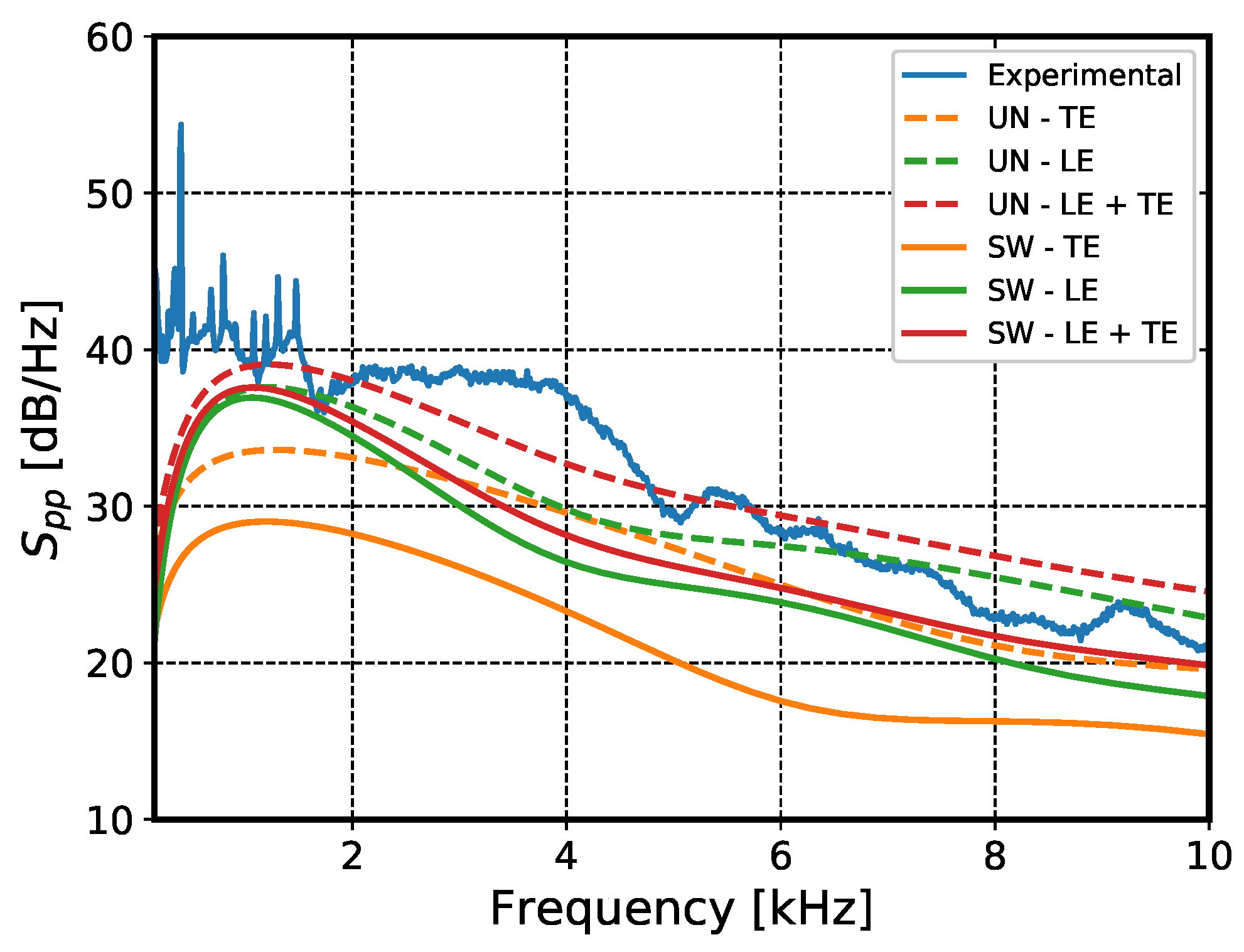
The acoustic far-field predicted results are compared in Figure 12 with the measured spectrum of the fan at its nominal operating condition. The experimental sound curve presents tonal contributions, particularly at the blade-passing frequency (around 400 Hz) and its harmonics not accounted for in the prediction methodology. When including the sweep-angle effect, the LE noise mechanism appears to be relevant throughout the all frequency spectrum, while still being comparable to the TE noise around 3.75 kHz and at very high frequencies. This is in agreement with the rotating beamforming result, on the same automotive fan, at the same working condition investigated by Amoiridis et al. [48] (see Figure 13), as well as with the results of Herold et al. [9]. The unswept behavior is fairly similar to the one computed in Figure 10 by Sanjose and Moreau in [12], on a similar but less forward-skewed automotive fan (H380EC1). We can affirm that the sum of the LE and TE sound mechanisms for the swept formulation is in fairly good agreement with the experimental curve, especially at high frequency, resulting in a better description of the noise emission with respect to the unswept classical Amiet’s formulation. The unswept case instead, overpredicts the radiated noise in this frequency range. As expected, the methodology is not suited to model the sound spectrum for very low-frequencies; in this region, most of the radiated sound is generated by subharmonic coherent vortical structures convected upstream within the gap between the fan shroud and the rotating ring [23,24]. Secondary flows with more broadband behavior as well as recirculation bubbles under the trailing-edge pressure side of the blade can also take place in the tip and near the hub regions [25], but their modeling would require higher-order CFD inputs to feed the semianalytical methods.

5.4. Sensitivity Study

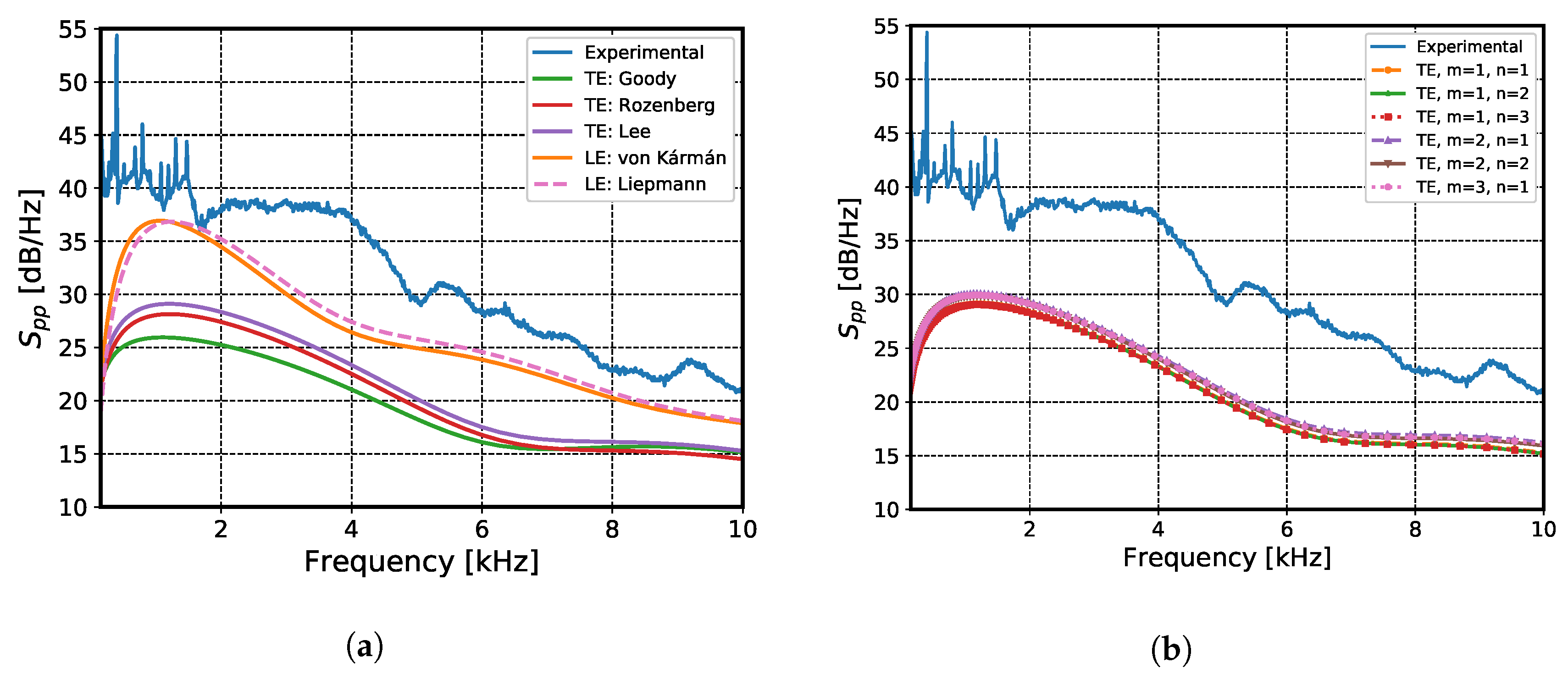
In Figure 12, the von Kármán’s model, Lee’s model, and the original Corcos’ model with $m=1$ and $n=1$ have been used to delineate the far-field results. Nevertheless, it is interesting to investigate which of the models proposed in Section 4 provide the best comparison with respect to the experimental far-field acoustics. Figure 13a shows that among the three semiempirical wall-pressure models, Lee’s and Rozenberg’s better compare with respect to Goody’s, the latter giving a PSD reduction of up to 3 dB. This is expected as Goody’s model does not account for the effect of adverse pressure gradients developing on the blades, and consequently underpredicts the low frequencies. This is consistent with the results reported by Sanjose and Moreau on the H380EC1 fan [12]. A negligible shift in frequency is encountered when employing the von Kármán’s or Liepmann’s models for the LE noise prediction, also in agreement with [12,49]. Several combinations of Butterworth-filter orders have been tested in Figure 13b, appearing to have a negligible effect on the TE noise prediction, with a relative difference of less than 1 dB.

6. Conclusions

We implemented a semianalytical methodology, based on Amiet’s theory, to predict the leading-edge and the trailing-edge noise mechanisms for an automotive fan with forward-skewed blades. The aim of the present work was to extend the low-order noise prediction methodology developed in [18], exploiting the same near-field steady RANS computation and comparing the results with the experimental ones. The blades have been divided into strips through isoradius cuts where the single-airfoil Amiet’s theory has been calculated, taking into account the local sweep angles for the leading and trailing edges separately.

The overall effect of considering swept blades with respect to the classical Amiet’s formulations is a reduction of the predicted noise for both sound mechanisms and throughout the all frequency spectrum. This mitigating effect is particularly efficient at the blade tip, where the highest values of local sweep angles are attained. In fact, the most emitting strips are found to be the ones within the interval $0.15<y/L_B<0.45$. A crucial consideration is that neglecting sweep effects can lead to the erroneous conclusion that the dominant strips are the ones at the tip of the blade, due to higher relative velocities, whereas in that area the forward curvature mitigates substantially the noise emission. Considering the sweep-angle effects also allows us to discern the relative importance between the LE and TE noise mechanisms, the former being globally dominant but comparable to the latter around 3.75 kHz and at very high frequencies, in agreement with [9,12,48].

A sensitivity analysis complements this work by studying three of the modeling key parameters. Firstly, the correct location at which one has to extract the CFD information to feed the LE noise model is proposed to be at 12% of the chord, upstream of the leading-edge location. Secondly, the semiempirical models that account for adverse pressure gradient flows are the best at comparing with the experimental results in agreement with [25]; specifically, Lee’s model exhibits the best trend. Thirdly, the relatively new Generalized Corcos’s model was implemented to calculate the spanwise integral length scale with a formulation that accounts for the coupled influence of the skewed wavenumbers on the spectral energy. Even though further investigations are required, the Butterworth-filter order coefficients seem to have a negligible influence on the far-field noise prediction.

References

- Moreau, S.; Roger, M. Advanced noise modeling for future propulsion systems. Int. J. Aeroacoust. 2018, 17, 576–599. [Google Scholar] [CrossRef]
- Allam, S.; Åbom, M. Noise reduction for automotive radiator cooling fans. In Proceedings of the FAN 2015, Lyon, France, 15–17 April 2015. [Google Scholar]
- Oerlemans, S. Reduction of wind turbine noise using blade trailing edge devices. In Proceedings of the 22nd AIAA/CEAS Aeroacoustics Conference, Lyon, France, 30 May–1 June 2016. [Google Scholar]
- Schäfer, R.; Böhle, M. Validation of the Lattice Boltzmann Method for Simulation of Aerodynamics and Aeroacoustics in a Centrifugal Fan. Acoustics 2020, 2, 735–752. [Google Scholar] [CrossRef]
- Metzger, F.B.; Rohrbach, C. Benefits of blade sweep for advanced turboprops. J. Propuls. Power 1986, 2, 534–540. [Google Scholar] [CrossRef]
- Henner, M.; Demory, B.; Franquelin, F.; Beddadi, Y.; Zhang, Z. Test Rig Effect on Performance Measurement for Low Loaded Large Diameter Fan for Automotive Application. In Volume 1A: Aircraft Engine; Fans and Blowers; American Society of Mechanical Engineers: Düsseldorf, Germany, 2014. [Google Scholar]
- Henner, M.; Demory, B.; Alaoui, M.; Laurent, M.; Behey, B. Effect of Blade Curvature on Fan Integration in Engine Cooling Module. Acoustics 2020, 2, 776–790. [Google Scholar] [CrossRef]
- Moreau, S.; Roger, M. Competing Broadband Noise Mechanisms in Low-Speed Axial Fans. AIAA J. 2007, 45, 48–57. [Google Scholar] [CrossRef]
- Herold, G.; Zenger, F.; Sarradj, E. Influence of blade skew on axial fan component noise. Int. J. Aeroacoust. 2017, 16, 418–430. [Google Scholar] [CrossRef]
- Roger, M.; Moreau, S.; Guedel, A. Broadband fan noise prediction using single-airfoil theory. Noise Control Eng. J. 2006, 54, 5–14. [Google Scholar] [CrossRef]
- Moreau, S. Turbomachinery Noise Predictions: Present and Future. Acoustics 2019, 1, 92–116. [Google Scholar] [CrossRef] [Green Version]
- Sanjosé, M.; Moreau, S. Fast and accurate analytical modeling of broadband noise for a low-speed fan. J. Acoust. Soc. Am. 2018, 143, 3103–3113. [Google Scholar] [CrossRef]
- Grasso, G.; Roger, M.; Moreau, S. Effect of sweep angle and of wall-pressure statistics on the free-field directivity of airfoil trailing-edge noise. In Proceedings of the 25th AIAA/CEAS Aeroacoustics Conference, Delft, The Netherlands, 20–23 May 2019. [Google Scholar]
- Roger, M.; Schram, C.; Moreau, S. On vortex–airfoil interaction noise including span-end effects, with application to open-rotor aeroacoustics. J. Sound Vib. 2014, 333, 283–306. [Google Scholar] [CrossRef]
- Rozenberg, Y.; Roger, M.; Moreau, S. Rotating Blade Trailing-Edge Noise: Experimental Validation of Analytical Model. AIAA J. 2010, 48, 951–962. [Google Scholar] [CrossRef] [Green Version]
- Amiet, R. Acoustic radiation from an airfoil in a turbulent stream. J. Sound Vib. 1975, 41, 407–420. [Google Scholar] [CrossRef]
- Amiet, R. Noise due to turbulent flow past a trailing edge. J. Sound Vib. 1976, 47, 387–393. [Google Scholar] [CrossRef]
- Zarri, A.; Christophe, J.; Schram, C.F. Low-Order Aeroacoustic Prediction of Low-Speed Axial Fan Noise. In Proceedings of the 25th AIAA/CEAS Aeroacoustics Conference, Delft, The Netherlands, 20–23 May 2019; p. 2760. [Google Scholar]
- Lee, S. Empirical Wall-Pressure Spectral Modeling for Zero and Adverse Pressure Gradient Flows. AIAA J. 2018, 56, 1818–1829. [Google Scholar] [CrossRef]
- Corcos, G.M. The structure of the turbulent pressure field in boundary-layer flows. J. Fluid Mech. 1964, 18, 353–379. [Google Scholar] [CrossRef]
- Roger, M.; Moreau, S. Back-scattering correction and further extensions of Amiet’s trailing-edge noise model. Part 1: Theory. J. Sound Vib. 2005, 286, 477–506. [Google Scholar] [CrossRef]
- Caiazzo, A.; D’Amico, R.; Desmet, W. A Generalized Corcos model for modelling turbulent boundary layer wall pressure fluctuations. J. Sound Vib. 2016, 372, 192–210. [Google Scholar] [CrossRef]
- Magne, S.; Moreau, S.; Berry, A. Subharmonic tonal noise from backflow vortices radiated by a low-speed ring fan in uniform inlet flow. J. Acoust. Soc. Am. 2015, 137, 228–237. [Google Scholar] [CrossRef]
- Moreau, S.; Sanjose, M. Sub-harmonic broadband humps and tip noise in low-speed ring fans. J. Acoust. Soc. Am. 2016, 139, 118–127. [Google Scholar] [CrossRef]
- Sanjose, M.; Lallier-Daniels, D.; Moreau, S. Aeroacoustic Analysis of a Low-Subsonic Axial Fan. In Volume 1: Aircraft Engine; Fans and Blowers; Marine; ASME: Montreal, QC, Canada, 2015. [Google Scholar]
- Bilka, M.; Anthoine, J.; Schram, C. Design and evaluation of an aeroacoustic wind tunnel for measurement of axial flow fans. J. Acoust. Soc. Am. 2011, 130, 3788–3796. [Google Scholar] [CrossRef]
- Menter, F.R. Two-equation eddy-viscosity turbulence models for engineering applications. AIAA J. 1994, 32, 1598–1605. [Google Scholar] [CrossRef] [Green Version]
- Sreenivasan, K.R. On the universality of the Kolmogorov constant. Phys. Fluids 1995, 7, 2778–2784. [Google Scholar] [CrossRef] [Green Version]
- Versteeg, H.K.; Malalasekera, W. An Introduction to Computational Fluid Dynamics: The Finite Volume Method, 2nd ed.; Pearson Education Ltd.: Harlow, UK; New York, NY, USA, 2007. [Google Scholar]
- Schlinker, R.; Amiet, R. Helicopter rotor trailing edge noise. In Proceedings of the 7th Aeroacoustics Conference, Palo Alto, CA, USA, 5–7 October 1987; AIAA: Palo Alto, CA, USA, 1981. [Google Scholar]
- Sinayoko, S.; Kingan, M.; Agarwal, A. Trailing edge noise theory for rotating blades in uniform flow. Proc. R. Soc. A Math. Phys. Eng. Sci. 2013, 469, 20130065. [Google Scholar] [CrossRef]
- Giez, J.; Vion, L.; Roger, M.; Moreau, S. Effect of the Edge-and-Tip Vortex on Airfoil Selfnoise and Turbulence Impingement Noise. In Proceedings of the 22nd AIAA/CEAS Aeroacoustics Conference, Lyon, France, 30 May–1 June 2016; AIAA: Lyon, France, 2016. [Google Scholar]
- Roger, M.; Carazo, A. Blade-Geometry Considerations in Analytical Gust-Airfoil Interaction Noise Models. In Proceedings of the 16th AIAA/CEAS Aeroacoustics Conference, Stockholm, Sweden, 7–9 June 2010. [Google Scholar]
- Rozenberg, Y. Modélisation Analytique du Bruit AéRodynamique à Large Bande des Machines Tournantes: Utilisation de Calculs MoyennéS de MéCanique des Fluides. Ph.D. Thesis, Ecole Centrale de Lyon, Ecully, France, 2007; p. 190. [Google Scholar]
- Christophe, J.; Anthoine, J.; Moreau, S. Amiet’s Theory in Spanwise-Varying Flow Conditions. AIAA J. 2009, 47, 788–790. [Google Scholar] [CrossRef]
- Christophe, J. Application of Hybrid Methods to High Frequency Aeroacoustics. Ph.D. Thesis, Universite Libre de Bruxelles, Brussels, Belgium, 2011. [Google Scholar]
- Volkmer, K.; Carolus, T. Correction: Aeroacoustic airfoil shape optimization utilizing semi-empirical models for trailing edge noise prediction. In Proceedings of the 2018 AIAA/CEAS Aeroacoustics Conference, Atlanta, GA, USA, 25–29 June 2018; American Institute of Aeronautics and Astronautics: Atlanta, GA, USA, 2018. [Google Scholar] [CrossRef]
- Goody, M. Empirical Spectral Model of Surface Pressure Fluctuations. AIAA J. 2004, 42, 1788–1794. [Google Scholar] [CrossRef]
- Küçükosman, Y.C.; Christophe, J.; Schram, C. Trailing edge noise prediction based on wall pressure spectrum models for NACA0012 airfoil. J. Wind Eng. Ind. Aerodyn. 2018, 175, 305–316. [Google Scholar] [CrossRef]
- Chase, D.M. Turbulent Boundary Layer Wall Pressure. J. Sound Vib. 1980, 70, 29–67. [Google Scholar] [CrossRef]
- Howe, M.S. Acoustics of Fluid-Structure Interactions, 1st ed.; Cambridge University Press: Cambridge, UK, 1998. [Google Scholar]
- Bradshaw, P.; Ferriss, D.H. Applications of a General Method of Calculating Turbulent Shear Layers. J. Basic Eng. 1972, 94, 345–351. [Google Scholar] [CrossRef]
- Rozenberg, Y.; Robert, G.; Moreau, S. Wall-Pressure Spectral Model Including the Adverse Pressure Gradient Effects. AIAA J. 2012, 50, 2168–2179. [Google Scholar] [CrossRef] [Green Version]
- Zagarola, M.V.; Smits, A.J. Mean-flow scaling of turbulent pipe flow. J. Fluid Mech. 1998, 373, 33–79. [Google Scholar] [CrossRef]
- Clauser, F.H. Turbulent Boundary Layers in Adverse Pressure Gradients. J. Aeronaut. Sci. 1954, 21, 91–108. [Google Scholar] [CrossRef]
- Coles, D. The law of the wake in the turbulent boundary layer. J. Fluid Mech. 1956, 1, 191–226. [Google Scholar] [CrossRef] [Green Version]
- Durbin, P.A.; Pettersson Reif, B.A. Statistical Theory and Modeling for Turbulent Flows; John Wiley & Sons, Ltd.: Hoboken, NJ, USA, 2011. [Google Scholar]
- Amoiridis, O.; Zarri, A.; Zamponi, R.; Christophe, J.; Schram, C.F.; Yakhina, G.; Moreau, S. Experimental Analysis of the Sound Radiated by an Automotive Cooling Module Working at Different Operational Conditions. In AIAA AVIATION 2020 FORUM; American Institute of Aeronautics and Astronautics: Reston, VA, USA, 2020. [Google Scholar] [CrossRef]
- Guérin, S.; Kissner, C.; Seeler, P.; Blázquez, R.; Carrasco Laraña, P.; de Laborderie, H.; Lewis, D.; Chaitanya, P.; Polacsek, C.; Thisse, J. ACAT1 Benchmark of RANS-Informed Analytical Methods for Fan Broadband Noise Prediction: Part II—Influence of the Acoustic Models. Acoustics 2020, 2, 617–649. [Google Scholar] [CrossRef]
Figure 1.
The relative velocity is plotted for an unsteady DES computation onto the isosurface obtained with the Q-criterion technique; large vortical structures are depicted in particular close to the ring and in the trailing-edge recirculating region near the hub.
Figure 2.
(a) ALCOVES anechoic chamber: upstream room with B&K microphones and open-rotor
configuration from [18]. (b) Suction-side 3D CAD model of the Valeo forward-skewed fan employed in
the steady RANS simulation.
Figure 3.
The RANS-based numerical results show similar azimuthal features over the
7 non-equally-distributed fan blades, making it possible to deal with them separately: in (a), the relative
velocity is illustrated on a plane normal to the fan rotating axis, showing higher velocities at the blade
trailing-edge tips; in (b), the distribution of pressure indicates that the most loaded zones are the blade
leading-edge tips.
Figure 4.
Inlet turbulence parameters are extracted from the steady-RANS computation in upstream
of the blade leading-edge line and depicted as functions of the spanwise normalized distance y/LB:
in (a), the mean square of the velocity fluctuations
is depicted; in (b), the characteristic length scale
of the turbulent eddies
is illustrated.
Figure 5.
Three isoradial cuts are plotted at 3 spanwise locations y/LB: (a) the boundary-layer velocity
profiles are depicted as functions of the non-dimensional boundary-layer distance yc/c with the red
dots corresponding to the boundary layer thickness δ; (b) the negative pressure coefficient Cp is plotted
as function of the chordwise nondimensional coordinate xc/c.
Figure 6.
(a) From [15], the rotating local airfoil reference frame is denoted. The fixed reference frame
defines the observer’s position. (b) Sweep-angle definition over the leading edge of the
fan blade; the rotated local reference frame
is determined.
Figure 7.
For the leading-edge case, the blade is divided into 10 segments: in (a), a classical unswept
leading-edge formulation can be used; in (b), the effect of the sweep is evaluated with blade strips
which have locally parallel leading-edges, following the blade forward-skewed curvature.
Figure 8.
For the trailing-edge case, the blade is divided into 10 segments: in (a), a classical unswept
trailing-edge formulation can be used; in (b), the effect of the sweep is evaluated with blade strips
which have locally parallel trailing-edges, following the blade forward-skewed curvature.
Figure 9.
Convergence study on the number of strips to use in order to acceptably discretize the noise
sources on the blade span: (a) leading-edge noise prediction case, (b) trailing-edge noise prediction case.
Figure 10.
Far-field sound power-spectral density (PSD) distribution over the blade span. The dashed
curves represent the classical Amiet’s theory, whilst the solid ones take into account the varying
sweep-angle: (a) leading-edge noise prediction case, (b) trailing-edge noise prediction case.
Figure 11.
The turbulent kinetic energy content is shown in (a); colored concentric circles represent the
isoradial locations at which the blade is cut in order to study the overall SPL of the strips shown in (b).
Here, the overall SPL is depicted against the upstream chord distance from the leading-edge point.
Figure 12.
PSD of the far-field emitted sound by the fan at its nominal working point: the solid red line representing the summation of trailing-edge (TE) and leading-edge (LE) noise contributions for the swept case (SW) is in fairly good agreement with the experimental curve in solid blue, especially at high frequency, resulting into a better description of the noise emission with respect to the unswept (UN) classical Amiet’s formulation shown in dashed line. In this plot, Lee’s model and Corcos’ model with and are employed for the TE noise prediction, whilst the von Kármán’s model is used for the LE noise prediction.
Figure 13.
A parametric study is proposed for the SW case by comparing the predicted results with
the measured ones: in (a), 3 semiempirical wall-pressure models Lee’s, Rozenberg’s, and Goody’s are
compared for the TE case; 2 turbulence velocity fluctuations models: von Kármán’s and Liepmann’s
are compared for the LE case. In (b), several combinations of the Corcos’ order coefficients m and n are
tested out.
Publisher’s Note: MDPI stays neutral with regard to jurisdictional claims in published maps and institutional affiliations. |
© 2020 by the authors. Licensee MDPI, Basel, Switzerland. This article is an open access article distributed under the terms and conditions of the Creative Commons Attribution (CC BY) license (http://creativecommons.org/licenses/by/4.0/).
Share and Cite
MDPI and ACS Style
Zarri, A.; Christophe, J.; Moreau, S.; Schram, C. Influence of Swept Blades on Low-Order Acoustic Prediction for Axial Fans. Acoustics 2020, 2, 812-832. https://0-doi-org.brum.beds.ac.uk/10.3390/acoustics2040046
AMA Style
Zarri A, Christophe J, Moreau S, Schram C. Influence of Swept Blades on Low-Order Acoustic Prediction for Axial Fans. Acoustics. 2020; 2(4):812-832. https://0-doi-org.brum.beds.ac.uk/10.3390/acoustics2040046
Chicago/Turabian StyleZarri, Alessandro, Julien Christophe, Stéphane Moreau, and Christophe Schram. 2020. "Influence of Swept Blades on Low-Order Acoustic Prediction for Axial Fans" Acoustics 2, no. 4: 812-832. https://0-doi-org.brum.beds.ac.uk/10.3390/acoustics2040046