
Efficient Forced Response Computations of Acoustical Systems with a State-Space Approach


Department of Engineering Acoustics, Faculty V of Mechanical Engineering and Transport Systems, Technische Universität Berlin, Einsteinufer 25, 10587 Berlin, Germany
*
Author to whom correspondence should be addressed.
Acoustics 2021, 3(3), 581-593; https://0-doi-org.brum.beds.ac.uk/10.3390/acoustics3030037
Submission received: 16 July 2021
/
Revised: 6 August 2021
/
Accepted: 7 August 2021
/
Published: 11 August 2021
(This article belongs to the Special Issue Advanced Modelling, Simulations and Measurements for Sound Insulation in Buildings)
Abstract
:State-space models have been successfully employed for model order reduction and control purposes in acoustics in the past. However, due to the cubic complexity of the singular value decomposition, which makes up the core of many subspace system identification (SSID) methods, the construction of large scale state-space models from high-dimensional measurement data has been problematic in the past. Recent advances of numerical linear algebra have brought forth computationally efficient randomized rank-revealing matrix factorizations and it has been shown that these factorizations can be used to enhance SSID methods such as the Eigensystem Realization Algorithm (ERA). In this paper, we demonstrate the applicability of the so-called generalized ERA to acoustical systems and high-dimensional input data by means of an example. Furthermore, we introduce a new efficient method of forced response computation that relies on a state-space model in quasi-diagonal form. Numerical experiments reveal that our proposed method is more efficient than previous state-space methods and can even outperform frequency domain convolutions in certain scenarios.
1. Introduction
A large class of acoustical systems can be classified as linear time-invariant (LTI) processes. Commonly, these systems are described by impulse response models; however, for certain modelling tasks, state-space descriptions of LTI systems can be advantageous compared to classical representations via the impulse response because they provide access to powerful model order reduction (MOR) techniques [1,2] and concepts of control theory [3].
Reduced order models are indispensable in applications where computational resources are a limiting factor, e.g., in real-time applications or in applications where models are evaluated perpetually. MOR aims at lowering the computational complexity of models of large-scale dynamical systems whilst conserving the system characteristics. Exemplary acoustical applications exist in [4,5,6,7], where reduced order state-space models are derived from a finite element method (FEM) of coupled vibro-acoustic systems with Sommerfeld boundary conditions for the analysis of radiation characteristics in the time domain. The reduction of the model order effectively enables transient time domain simulations of coupled vibro-acoustical systems that would otherwise be computationally infeasible with full order finite element models. Likewise, the MOR capabilities of state-space models have been successfully utilized for the reduced description of large fluid pressure fields in the areas of fluid dynamics [8,9] and thermoacoustics [10,11,12]. These reduced descriptions enabled the employment of feedback control strategies, among other things.
Similarly, state-space models are used for the design of feedback controllers that mitigate unwanted noise in the field of active noise control. In [13], a state-space model of structural vibrations in a vehicle is formulated from a coupled modal base that stems from FEM. The vibrations are then actively damped by inertial shakers with a feedback controller which is calculated on basis of the state-space model. Different modelling and control strategies for noise reduction in an acoustic duct are studied in [14,15,16].
Furthermore, state-space models can be superior over impulse response models when it comes to so-called forced response computations, i.e., the computation of the system output under given input excitations. As is demonstrated by means of a vibrating plate model in [17], state-space models are faster and more memory efficient than frequency domain convolutions if the output behaviour of the system is governed by a low number of poorly damped modes. The suitability and computational efficiency of state-space models has been studied further in the context of auralization [18,19]. In [20,21], state-space models are derived from head-related transfer function (HRTF) measurements. It is shown that the cost of forced response computations is much lower compared to finite impulse response filter arrays when combined with a model order reduction scheme. Due to the fact that the individual HRTFs have similar structure and are jointly described by a single state-space model, a reduction of model order is possible without compromising the reproduction quality.
Regardless of the use-case, state-space models can be obtained in different ways, either from physical knowledge of the system or from measurements. The former includes the construction of state-space models by discretization of the underlying differential equations or by associating the system modes with a dedicated states. The construction of state-space models from measurements belongs to the category of subspace system identification (SSID) problems. Depending on the kind of measurement data, there exist different algorithms such as the Eigensystem Realization Algorithm (ERA) [22], also known as Kung’s method [23], for impulse response data, as well as different SSID methods [24,25] for input-output data.
Several SSID algorithms, including ERA, rely on a singular value decomposition (SVD) [26] of the Hankel matrix, which makes them unfeasible for high-dimensional measurement data because of the cubic complexity of the SVD. Unlike HRTFs, general acoustic systems can have a much slower decay which implies longer impulse response measurements. Therefore, a measurement-based approach to state-space modelling was only possible for a limited set of LTI systems in the past. However, a generalized version of ERA has recently been introduced in [27,28] that replaces the SVD by an arbitrary orthogonal decomposition. This paves the way for the employment of highly efficient randomized rank-revealing matrix factorizations such as the CUR decomposition [29] or randomized SVD [30]. These low-rank approximations have a much lower memory demand and computational cost at an oftentimes negligible error increase. The computational cost can be reduced even further, when specialized matrix vector multiplication routines are incorporated that account for the structure of the Hankel matrix [26,28,31].
In this work, we demonstrate the applicability of generalized ERA with randomized SVD to acoustical systems by applying it to room impulse response (RIR) measurements. Furthermore, we show that state-space descriptions of acoustic LTI systems can be beneficial not only for MOR or system control but also for the computation of forced responses, because they can constitute computational savings compared to (frequency domain) convolutions.
The remainder of this paper is structured as follows: The subsequent Section gives a brief introduction into state-space descriptions and outlines the SSID method that will be used to construct state-space models from impulse response measurements. After that, approximations of the computational costs for different methods of forced response calculations are derived and we introduce a new efficient method of forced response calculation that is based on a state-space model in quasi-diagonal form. Section 3 introduces the measurement data that is used for the exemplary validation of the method. The quality of the identified models and the computational costs of forced response computations are presented in Section 4. Finally, the results are discussed in Section 5 and Section 6 concludes the paper.
2. Methods
2.1. State-Space Descriptions
Let denote the Hilbert space of square summable sequences. Any discrete-time LTI system with inputs and outputs is fully determined by its (matrix-valued) impulse response, i.e., the sequence
where , are the so-called Markov Parameters. For any input , we define the output by the convolution sum
Alternatively, a system can be described by the so-called state equations, a set of first-order linear difference equations of the form:
where is the so-called state of the system at time index , is called the (state) dimension of the system, the state matrix, the input map, the output map and the feedthrough matrix. For causal systems, the Markov parameters are then given by:
An important property of state-space systems is their invariance to similarity transformations. In other words, the transfer function and, equally, the Markov parameters of a system defined by the matrix quadruple are identical to those of the transformed system , where is an invertible matrix. This can be easily seen by plugging the transformed system into (3) and it is also intuitively clear, since the state of a system may be represented in different coordinate frames without changing its input-to-output behaviour.
2.2. Generalized ERA
We will now introduce ERA, the SSID method that is applied in this paper. Given measurements of the first , Markov parameters , , the so-called Hankel matrix is given by:
The Hankel matrix is of system theoretical relevance [1] and plays an important role in SSID. By plugging (3) into (4), the Hankel matrix can be factored into
the so-called observability matrix and controllability matrix . From this factorization, the matrix quadruple that defines the underlying system can be derived. In ERA, the system matrices B and C are directly read from and , whereas the state matrix A is obtained by computing a least-squares solution to
where the superscripts f and l denote the submatrix consisting of the first and last rows respectively. A so-called partial realization is then given by
where denotes the Moore-Penrose inverse. In the standard version of ERA [22], a factorization of the form (5) is obtained by an SVD of the Hankel matrix, i.e.,
and the diagonal entries of are called the Hankel singular values of the system. The observability and controllability matrices can then simply be chosen as
It has been proven in [27] that the SVD from (6) can be replaced by an arbitrary orthogonal rank approximation of the Hankel matrix such that the resulting realization approximates the system and that stability is retained under the same assumptions as Kung’s original method [23]. This technique is called the generalized ERA. In the following sections, we use generalized ERA in conjunction with the randomized SVD [30] as suggested in [28].
2.3. Forced Response Computations
In certain applications it may be necessary to compute the forced response of an LTI system. Towards that goal, let be an input sequence of length and assume that the system has inputs and outputs and that it is fully determined by Markov parameters. It then follows that any output sequence has at most non-zero entries.
There exist several strategies for the computation of the output y, some of which we will compare in regards to the computational cost in the following. The computational cost is defined as the number of floating point operations (flops), i.e., the number floating point additions and multiplications, that are required to compute every sample of the output y. For the classical time domain convolution according to (1), the cost is given by
In certain scenarios, e.g., if s and l are both large, the cost can become relatively high. To remedy this, the convolution is oftentimes performed in the frequency domain. For this, the input u and the single-channel impulse responses , , , are zero-padded to length and then transformed into the frequency domain by two real-to-complex discrete Fourier transforms (DFTs). The elementwise product of the complex spectra is formed and the result is transformed back into the time domain by a complex-to-real DFT. Both DFT variants need at least flops (for inputs of length , , this bound is exact) with the standard Radix-2 FFT algorithm [32]. Together with a cost of 6 flops per complex multiplication, this yields a minimal total cost of
for signals that are not necessarily of length . A drawback of the DFT approach is that it is not possible to pursue sample-wise stream processing schemes, because the input signals and impulse responses have to be transformed wholly. For real time applications, there exist block-partitioned frequency domain processing schemes that can be implemented at additional computational costs [33]. Looking at (7) and (8), it can be seen that both convolution methods scale superlinearly if the signal length l and measurement length s are increased simultaneously. Furthermore, doubling both the number of inputs m and outputs p will quadruple the cost in both cases.
An interesting alternative to convolutions is presented by a state-space approach. If the forced response computations are carried out in state-space according to (2), the cost is given by
in absence of feedthrough, i.e., . The cost now scales linearly with the signal lengths s and l and a doubling of both m and p will also lead to double the cost. Furthermore, the output is computed sample-wise, which inherently suits real-time applications. On the downside, the computational cost now additionally depends on the state dimension n and scales quadratically with it. Quite possibly, the state-space approach is computationally cheaper than a frequency domain convolution, but for systems with slowly decaying Hankel singular values, the congruous state dimension may be very large which implies an increased cost and memory demand.
The computational cost of (9) can be improved upon by transformation of the state-space model such that the state matrix A is in quasi-triangular form as suggested in [20,21]. With the Schur decomposition [26], every square matrix can be expressed as , where is orthogonal and is quasi-triangular. Hence, the cost of multiplying with the state matrix of the transformed system is reduced from a dense matrix-vector multiplication with flops to a Hessenberg matrix-vector multiplication with flops such that for the overall cost it holds:
Compared to (9), the computations are accelerated by a factor of roughly two, but the complexity still scales quadratically with n.
In this paper, we propose to take this conception even further and diagonalize the state matrix by means of an eigendecomposition [26]. It states that every non-defective matrix can be written as , where is a regular matrix containing the eigenvectors of A and is a diagonal matrix containing the complex eigenvalues of A. For such a decomposition, there exists a regular matrix , such that for and it holds
where has so-called quasi-diagonal structure, i.e., a block-diagonal matrix with real diagonal blocks , of size one or two that correspond to the complex eigenvalues , of A. For every real eigenvalue, the corresponding diagonal block is of size one and identical to the real eigenvalue. Since the complex eigenvalues of real matrices come in conjugated pairs, every pair of complex eigenvalues corresponds to a block with the real part of the eigenvalues on the diagonal and the imaginary parts on the antidiagonal. The state transformation with now yields a system in so-called canonical quasi-diagonal form and a multiplication with the state matrix can now be efficiently realized by a tridiagonal matrix-vector multiplication which implies that the overall cost now scales linearly with the state dimension n:
Note that although a state transformation with would yield a diagonal state matrix, the overall computational cost with a tridiagonal but real state matrix is lower, because complex arithmetic is avoided. However, if the processor has a specialized instruction set for complex arithmetic, a diagonal transformation may be adequate.
An overview over the computational complexities and storage costs of the previously presented methods is given in Table 1. For minimal realizations of causal discrete-time systems, the state-dimension n is bounded by s, which suggests that the scaling of our method is superior in both computational and storage costs over all other presented methods. This is especially the case if the system has a large number of inputs and outputs. However, a transformation into (quasi-)diagonal form is only possible if the state matrix is non-defective.
3. Example
3.1. Database
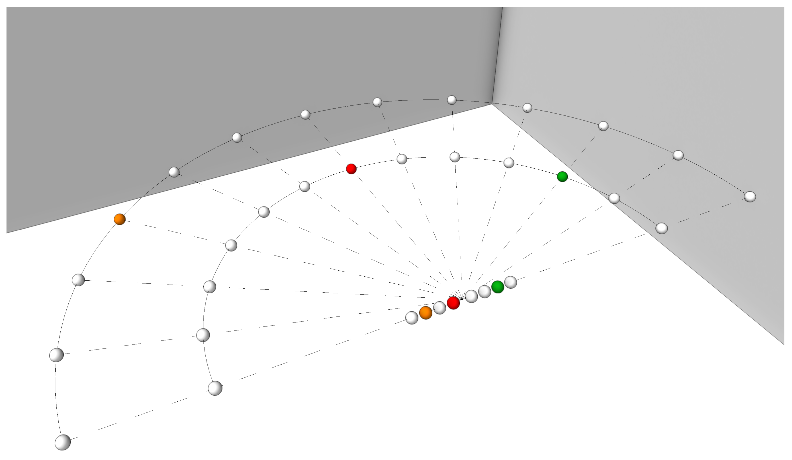
The SSID method outlined in Section 2.2 is applicable to arbitrary acoustical LTI systems. In the following, we will use it for the identification of a room acoustical system with measurement data from the Multichannel Impulse Response Database [34]. The database provides RIR measurements from sources that are distributed evenly over two semicircles to a linear microphone array with microphones which results in a total of 208 measurements for different reverberation and microphone array configurations. For the exemplary application in the following, we choose the scenario in which the room reverberation time was set to and the microphone spacings of the array were configured to . The geometric setup of the source and microphone arrangement is visualized in Figure 1 [34].
3.2. Preprocessing
The RIR measurements have a duration of 10 s at a sampling rate of . In order to avoid unnecessary computations, the RIR measurements are preprocessed such that only relevant information is contained in the input data. For this, the common delay among the measurements of approximately is removed and the RIRs are truncated to a total duration of which equals the reverberation time of the room. As stated in [34], the measurement speakers are only linear in the range of to . Therefore, after truncation, the RIRs are downsampled by a factor of two, which reduces the sampling rate to and the Nyquist frequency to . As a result, we use 208 RIRs with a length of samples as input to our method. Lastly, the RIRs are normalized such that
With this normalization, the energy of the single-channel transmissions will be approximately equal to one:
4. Results
After constructing the matrix-valued Markov parameters from the individual preprocessed RIRs, a rank 2000 approximation of the Hankel matrix was computed with randomized SVD [30]. Due to the implementation of a dedicated matrix-vector multiplication routine that exploits the Hankel structure [28,31], the full construction of the Hankel matrix was circumvented and the computations could easily be carried out on an Intel® Core™ i5-9400F CPU @ with of memory in under six minutes. In our example, the Hankel matrix has a size of 30,720 × 99,840 which would already require about of memory to explicitly construct. In contrast, the storage of the Markov parameters only required and the randomized rank 2000 SVD required about of memory in our case.
This rank 2000 decomposition served as a basis for the construction of all subsequent models. Firstly, a “full” realization with dimension 2000 was obtained by generalized ERA as described in Section 2.2 and partial realizations were constructed in a similar fashion but only taking the first 1000, 500 and 120 singular values and singular vectors as input, respectively. Additionally, a frequency-limited partial realization was obtained by MOR of the “full” realization with a frequency-limited Balanced Truncation along the lines of [35]. A frequency range of 100–1000 Hz was chosen for this realization together with a reduced model order of 120.
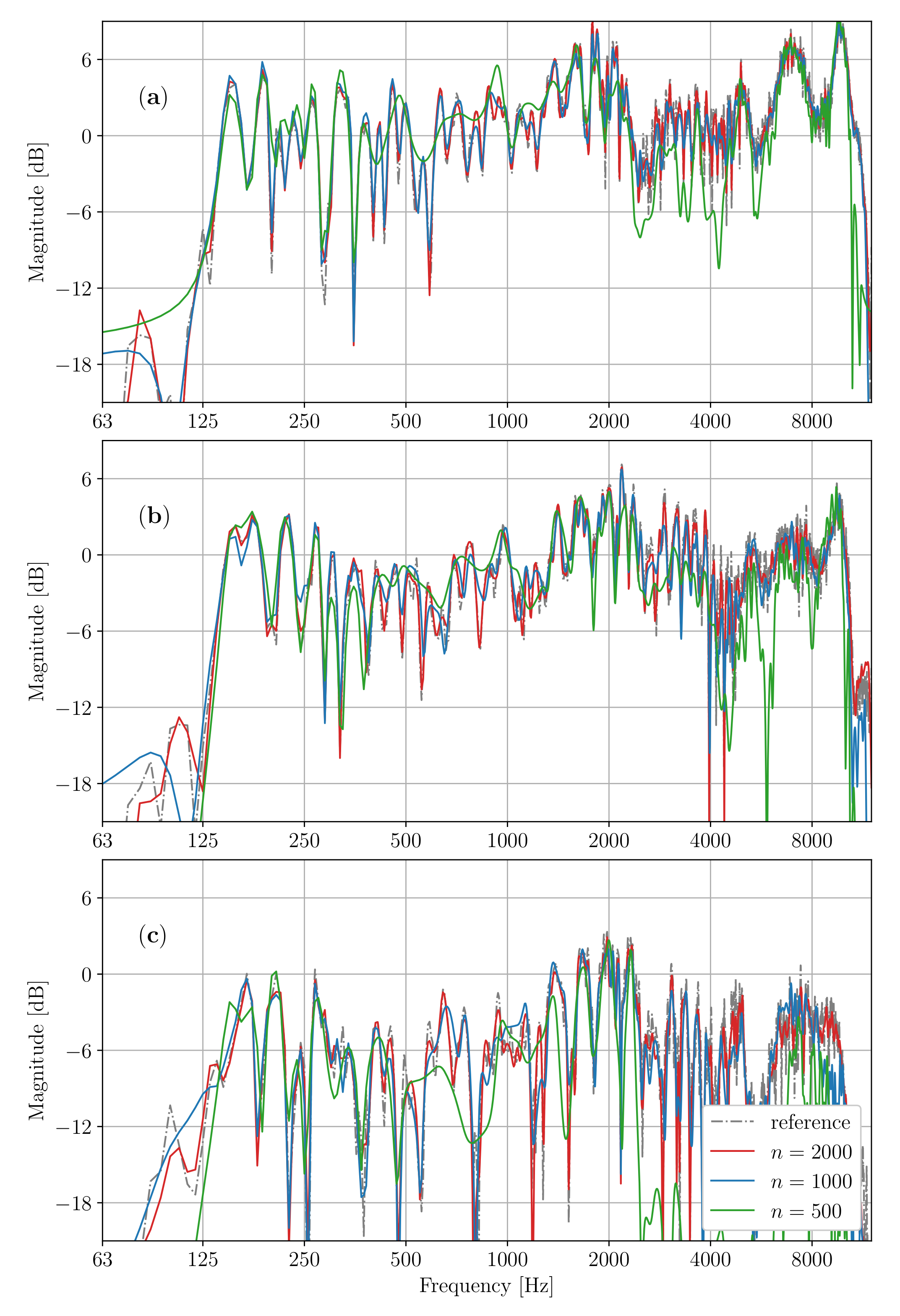
The single-channel magnitude responses of the three largest models are depicted in Figure 2 together with the magnitudes of the Fourier transform of the corresponding RIRs. Since we do not have access to the frequency dependent singular values of the transfer function of the room acoustical system, a comparison of the single-channel magnitude responses is feasible. The reproduction quality of the models is virtually identical across all 208 channels, which is why we limit the depiction to three arbitrarily selected channels. The magnitude responses of the order 2000 model are in very good agreement with the measurements across all frequencies. Decreasing the model order to 1000 still yields plausible approximations of the reference magnitudes, whereas the magnitudes of the model with order 500 exhibit more drastic deviations of the reference magnitude sporadically.
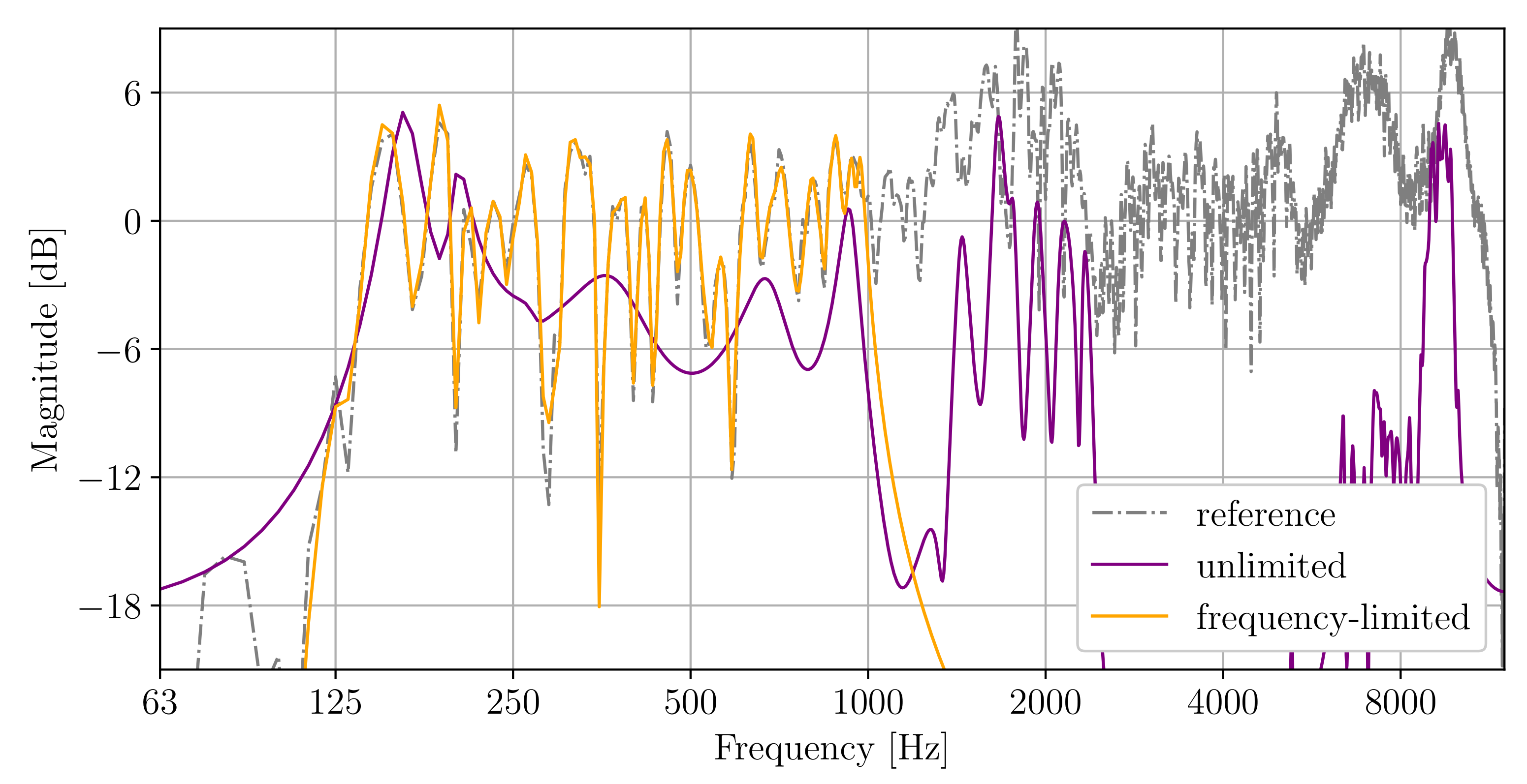
Figure 3 shows the single-channel magnitude responses of the models with order 120. Since, again, the reproduction quality is the same for all 208 channels, only one transmission channel is depicted. It can be clearly seen that the unlimited model is not capable of reproducing the reference magnitude response. In contrast, the frequency-limited model does so nearly perfectly in the given frequency range. Since the frequency-limited model stems from the “full” order 2000 realization, its model error is bounded by the “full” model. Seeing that the remaining small deviations of the frequency-limited model are also present in the order 2000 realization, it seems likely that the frequency-limited model could be even further improved upon if it was based on an even larger approximate factorization of the Hankel matrix.
Table 2 contains the -norms of the approximation error and frequency-limited approximation error
where denotes the RIR measurements, denotes the impulse response of the realization and denotes the frequency-limited Fourier transform with frequency interval , i.e.,
for . As mentioned above, we do not have access to the true system realization, hence we cannot compute the classical approximation errors in terms of norms of Hardy spaces such as the (frequency-limited) or norms. Instead, we consult the norm which is virtually identical to the norm.
With these models, forced response computations were carried out with the methods introduced in Section 2.3. A random input of duration, i.e., l = 24,000, was used in all cases and the required flops were measured with the Performance Application Programming Interface [36]. An overview of the theoretical costs and the required flops for the realizations, as well as the classical convolution methods, is given in Table 3. The computations were carried out in the Python programming language (v.3.9.4), for the convolutions we have made recourse to the respective SciPy (v.1.6.3) implementations [37]. The last column of the table shows the condition number of the state-space transformation Y. In case of the Schur decomposition, Y is orthogonal and its condition is always equal to one. For the (quasi-)diagonal transformation, the condition depends on the structure of the eigenvectors of A.
5. Discussion
The results of the previous show that the approximation error can be improved by increasing the model order (see Table 2) and that the identification of large realizations is possible on consumer grade computers. An example of a frequency-limited realization was included in order to emphasize the potential of a state-space approach when the model is truncated such that it solely captures necessary information. Similar approaches exist which allow for time-limited MOR [35,38].
We have validated the derived cost bounds for different methods of forced response computations with numerical experiments. For the state-space methods, the required flops were slightly higher than the derived bounds (see Table 3). This can be explained by additional computational overhead that is not captured in the idealized bounds. Contrarily, the required flops for the convolutions were lower than the derived bounds which is probably due to the highly optimized convolution routines of the SciPy package. For the large order 2000 model, the DFT-based convolution was the fastest among all methods, but our method was already more than 8 times faster than a classical convolution in the time domain. In contrast, the other two state-space methods were at least 3 times slower than the latter. In the frequency-limited case, our method outperformed the DFT-based convolution and was faster by a factor of about .
It is difficult to achieve a meaningful juxtaposition of a state-space approach and DFT-based convolution, because, as mentioned earlier, the output is computed sample-per-sample with a state-space approach and DFT-based convolution relies on the transformation of the entire signal or overlapping blocks. Therefore, even large scale state-space models can be advantageous for forced response calculations in real-time applications where latency is important. Oftentimes, real-time applications go hand-in-hand with limited computational resources. This problem is also remedied by state-space models, because the model order can be reduced to a point that fully exhausts the computational resources available.
As mentioned in Section 2.3, the state-matrix A can only be transformed into diagonal form if it is non-defective. A sufficient condition for A to be non-defective is that it possesses only distinct eigenvalues. Pragmatically speaking, it is highly unlikely that A will have repeated eigenvalues, since it is computed from measurement data. Even if, say, the measurement points in our example were arranged in a symmetrical fashion, the presence of measurement noise alone would disturb the eigenvalues of A enough for A to be non-deficient. It should be noted, that even a formally non-defective state matrix can lead to ill-conditioned state transformations if the state matrix is close to a defective matrix [39]. Therefore, the condition number of the state-transformation Y is provided in Table 3 as an a-posteriori measure of the “defectiveness” of A. From our observations, there seems to be a connection to the decay of the Hankel singular values, where the condition number of Y increases as the decay of the Hankel singular values slows down. From a mathematical standpoint, this connection is not immediately clear and this remains an interesting research direction for the future. However, the encountered condition numbers are still acceptable in our example. Furthermore, if the decay of the Hankel singular value is slow, the model order can be simply reduced further such that the condition of Y improves.
6. Conclusions
We have successfully constructed large state-space models of a room-acoustical example system from impulse response measurements with generalized ERA [28,40]. Because the example system does not possess a special structure and is already quite complex, the applicability of generalized ERA also applies to general acoustical systems, not only room acoustical systems. Additionally, we have introduced a new efficient method of forced response computation that relies on a state-space model in (quasi-)diagonal form. In this way, this paper extends the works of [18,19,20,21] by using a generalized version of ERA with randomized SVD to be able to identify larger systems from high-dimensional measurement data and by enabling the forced response computations of such large models with our new more efficient method.
Author Contributions
Conceptualization, A.J.R.P. and E.S.; methodology, A.J.R.P.; software, A.J.R.P.; validation, A.J.R.P.; formal analysis, A.J.R.P.; investigation, A.J.R.P. and E.S.; resources, E.S.; data curation, A.J.R.P.; writing—original draft preparation, A.J.R.P.; writing—review and editing, E.S.; visualization, A.J.R.P.; supervision, E.S.; project administration, E.S.; funding acquisition, A.J.R.P. and E.S. All authors have read and agreed to the published version of the manuscript.
Funding
This research received no external funding.
Data Availability Statement
The code is available under https://0-doi-org.brum.beds.ac.uk/10.5281/zenodo.5167288 (accessed on 11 August 2021). The input data for the exemplary application in this study are openly available at https://www.iks.rwth-aachen.de/en/research/tools-downloads/databases/multi-channel-impulse-response-database (accessed on 11 August 2021).
Conflicts of Interest
The authors declare no conflict of interest.
Abbreviations
The following abbreviations are used in this manuscript:
| DFT | Discrete Fourier Transform |
| ERA | Eigensystem Realization Algorithm |
| FEM | Finite Element Method |
| FFT | Fast Fourier Transform |
| HRTF | Head-related Transfer Function |
| LTI | Linear Time-invariant |
| MOR | Model Order Reduction |
| RIR | Room Impulse Response |
| SSID | Subspace System Identification |
| SVD | Singular Value Decomposition |
References
- Antoulas, A.C. Approximation of Large-Scale Dynamical Systems; Advances in Design and Control; Society for Industrial and Applied Mathematics: Philadelphia, PA, USA, 2005. [Google Scholar]
- Gugercin, S.; Antoulas, A.C. A Survey of Model Reduction by Balanced Truncation and Some New Results. Int. J. Control 2004, 77, 748–766. [Google Scholar] [CrossRef]
- Zhou, K.; Doyle, J.C.; Glover, K. Robust and Optimal Control; Prentice Hall: Upper Saddle River, NJ, USA, 1996. [Google Scholar]
- Van Ophem, S.; Atak, O.; Deckers, E.; Desmet, W. Application of a Time-Stable Model Order Reduction Scheme to an Exterior Vibro-Acoustic Finite Element Model. In Proceedings of the ISMA 2016, Leuven, Belgium, 19–21 September 2016; p. 14. [Google Scholar]
- Van de Walle, A.; Shiozawa, Y.; Matsuda, H.; Desmet, W. Model Order Reduction for the Transient Vibro-Acoustic Simulation of Acoustic Guitars. In Proceedings of the ISMA 2016, Leuven, Belgium, 19–21 September 2016; p. 12. [Google Scholar]
- Van de Walle, A.; Naets, F.; Deckers, E.; Desmet, W. Stability-Preserving Model Order Reduction for Time-Domain Simulation of Vibro-Acoustic FE Models. Int. J. Numer. Meth. Eng. 2017, 109, 889–912. [Google Scholar] [CrossRef]
- Van Ophem, S.; Deckers, E.; Desmet, W. Parametric Model Order Reduction without a Priori Sampling for Low Rank Changes in Vibro-Acoustic Systems. Mech. Syst. Signal Process. 2019, 130, 597–609. [Google Scholar] [CrossRef]
- Brunton, S.L.; Dawson, S.T.; Rowley, C.W. State-Space Model Identification and Feedback Control of Unsteady Aerodynamic Forces. J. Fluids Struct. 2014, 50, 253–270. [Google Scholar] [CrossRef] [Green Version]
- Ma, Z.; Ahuja, S.; Rowley, C.W. Reduced-Order Models for Control of Fluids Using the Eigensystem Realization Algorithm. Theor. Comput. Fluid Dyn. 2011, 25, 233–247. [Google Scholar] [CrossRef] [Green Version]
- Mangesius, H.; Polifke, W. A Discrete-Time, State-Space Approach for the Investigation of Non-Normal Effects in Thermoacoustic Systems. Int. J. Spray Combust. Dyn. 2011, 3, 331–350. [Google Scholar] [CrossRef]
- Illingworth, S.J. Acoustic State-Models Using a Wave Based Approach. In Proceedings of the 21st International Congress on Sound and Vibration 2014, ICSV 2014, Beijing, China, 13–17 July 2014; p. 8. [Google Scholar]
- Meindl, M.; Emmert, T.; Polifke, W. Efficient Calculation of Thermoacoustic Modes Utilizing State-Space Models. In Proceedings of the 23rd International Congress on Sound and Vibration, ICSV23, Athens, Greece, 10–14 July 2016; p. 9. [Google Scholar]
- De Oliveira, L.P.; Varoto, P.S.; Sas, P.; Desmet, W. A State-Space Modeling Approach for Active Structural Acoustic Control. Shock Vib. 2009, 16, 607–621. [Google Scholar] [CrossRef]
- Hull, A.J.; Radcliffe, C.J.; Southward, S.C. Global Active Noise Control of a One-Dimensional Acoustic Duct Using a Feedback Controller. J. Dyn. Syst. Meas. Control 1993, 115, 488–494. [Google Scholar] [CrossRef]
- Hong, J.; Akers, J.; Venugopal, R.; Lee, M.-N.; Sparks, A.; Washabaugh, P.; Bernstein, D. Modeling, Identification, and Feedback Control of Noise in an Acoustic Duct. IEEE Trans. Contr. Syst. Technol. 1996, 4, 283–291. [Google Scholar] [CrossRef] [Green Version]
- Petersen, C.D.; Fraanje, R.; Cazzolato, B.S.; Zander, A.C.; Hansen, C.H. A Kalman Filter Approach to Virtual Sensing for Active Noise Control. Mech. Syst. Signal Process. 2008, 22, 490–508. [Google Scholar] [CrossRef] [Green Version]
- Nijsse, G.; Verhaegen, M.; Schutter, B.D.; Westwick, D.; Doelman, N. State Space Modeling in Multichannel Active Control Systems. In Proceedings of the 1999 International Symposium on Active Control of Sound and Vibration, Ft. Lauderdale, FL, USA, 2–4 December 1999; Institute of Noise Control Engineering of the USA: Saddle River, NJ, USA, 1999; pp. 909–920. [Google Scholar]
- Georgiou, P.; Kyriakakis, C. Modeling of Head Related Transfer Functions for Immersive Audio Using a State-Space Approach. In Proceedings of the Conference Record of the Thirty-Third Asilomar Conference on Signals, Systems, and Computers (Cat. No.CH37020), Pacific Grove, CA, USA, 24–27 October 1999; Volume 1, pp. 720–724. [Google Scholar] [CrossRef] [Green Version]
- Georgiou, P.; Kyriakakis, C. A Multiple Input Single Output Model for Rendering Virtual Sound Sources in Real Time. In Proceedings of the 2000 IEEE International Conference on Multimedia and Expo, ICME2000, New York, NY, USA, 30 July–2 August 2000; Proceedings. Latest Advances in the Fast Changing World of Multimedia (Cat. No.00TH8532). Volume 1, pp. 253–256. [Google Scholar] [CrossRef]
- Adams, N.; Wakefield, G. Efficient Binaural Display Using MIMO State-Space Systems. In Proceedings of the 2007 IEEE International Conference on Acoustics, Speech and Signal Processing, ICASSP’07, Honolulu, HI, USA, 15–20 April 2007; Volume 1, pp. I-169–I-172. [Google Scholar] [CrossRef]
- Adams, N.H.; Wakefield, G.H. State-Space Synthesis of Virtual Auditory Space. IEEE Trans. Audio Speech Lang. Process. 2008, 16, 881–890. [Google Scholar] [CrossRef]
- Juang, J.N.; Pappa, R.S. An Eigensystem Realization Algorithm for Modal Parameter Identification and Model Reduction. J. Guid. Control Dyn. 1985, 8, 620–627. [Google Scholar] [CrossRef]
- Kung, S. A New Identification and Model Reduction Algorithm via Singular Value Decomposition. In Proceedings of the 12th Asilomar Conference on Circuits, Systems and Computers, Pacific Grove, CA, USA, 6–8 November 1978; pp. 705–714. [Google Scholar]
- Verhaegen, M.; Dewilde, P. Subspace Model Identification Part 1. The Output-Error State-Space Model Identification Class of Algorithms. Int. J. Control 1992, 56, 1187–1210. [Google Scholar] [CrossRef]
- Van Overschee, P.; de Moor, B. N4SID: Numerical Algorithms for State Space Subspace System Identification. IFAC Proc. Vol. 1993, 26, 55–58. [Google Scholar] [CrossRef]
- Golub, G.H.; Van Loan, C.F. Matrix Computations, 4th ed.; Johns Hopkins Studies in the Mathematical Sciences; The Johns Hopkins University Press: Baltimore, MD, USA, 2013. [Google Scholar]
- Kramer, B.; Gorodetsky, A.A. System Identification via CUR-Factored Hankel Approximation. SIAM J. Sci. Comput. 2018, 40, A848–A866. [Google Scholar] [CrossRef]
- Minster, R.; Saibaba, A.K.; Kar, J.; Chakrabortty, A. Efficient Algorithms for Eigensystem Realization Using Randomized SVD. SIAM J. Matrix Anal. Appl. 2021, 42, 1045–1072. [Google Scholar] [CrossRef]
- Friedland, S.; Mehrmann, V.; Miedlar, A.; Nkengla, M. Fast Low Rank Approximations of Matrices and Tensors. Electron. J. Linear Algebra 2011, 22, 1031–1048. [Google Scholar] [CrossRef] [Green Version]
- Halko, N.; Martinsson, P.G.; Tropp, J.A. Finding Structure with Randomness: Probabilistic Algorithms for Constructing Approximate Matrix Decompositions. SIAM Rev. 2011, 53, 217–288. [Google Scholar] [CrossRef]
- Lu, L.; Xu, W.; Qiao, S. A Fast SVD for Multilevel Block Hankel Matrices with Minimal Memory Storage. Numer. Algorithms 2015, 69, 875–891. [Google Scholar] [CrossRef]
- Van Loan, C. Computational Frameworks for the Fast Fourier Transform; Number Vol. 10 in Frontiers in Applied Mathematics; Society for Industrial and Applied Mathematics (SIAM): Philadelphia, PA, USA, 1992. [Google Scholar]
- Wefers, F. Partitioned Convolution Algorithms for Real-Time Auralization; Number Band 20 in Aachener Beiträge Zur Technischen Akustik; Logos Verlag Berlin GmbH: Berlin, Germany, 2015. [Google Scholar]
- Hadad, E.; Heese, F.; Vary, P.; Gannot, S. Multichannel Audio Database in Various Acoustic Environments. In Proceedings of the 2014 14th International Workshop on Acoustic Signal Enhancement (IWAENC), Juan-les-Pins, France, 8–11 September 2014; pp. 313–317. Available online: https://www.iks.rwth-aachen.de/en/research/tools-downloads/databases/multi-channel-impulse-response-database (accessed on 11 August 2021). [CrossRef]
- Gawronski, W.; Juang, J.N. Model Reduction in Limited Time and Frequency Intervals. Int. J. Syst. Sci. 1990, 21, 349–376. [Google Scholar] [CrossRef]
- Barry, D.; Danalis, A.; Jagode, H. Effortless Monitoring of Arithmetic Intensity with PAPI’s Counter Analysis Toolkit. In Tools for High Performance Computing 2018/2019; Mix, H., Niethammer, C., Zhou, H., Nagel, W.E., Resch, M.M., Eds.; Springer International Publishing: Cham, Switzerland, 2021; pp. 195–218. [Google Scholar] [CrossRef]
- SciPy 1.0 Contributors; Virtanen, P.; Gommers, R.; Oliphant, T.E.; Haberland, M.; Reddy, T.; Cournapeau, D.; Burovski, E.; Peterson, P.; Weckesser, W.; et al. SciPy 1.0: Fundamental Algorithms for Scientific Computing in Python. Nat. Methods 2020, 17, 261–272. [Google Scholar] [CrossRef] [PubMed] [Green Version]
- Benner, P.; Werner, S.W. Frequency- and Time-Limited Balanced Truncation for Large-Scale Second-Order Systems. Linear Algebra Appl. 2021, 623, 68–103. [Google Scholar] [CrossRef]
- Akinola, R.O.; Freitag, M.A.; Spence, A. The Calculation of the Distance to a Nearby Defective Matrix. Numer. Linear Algebra Appl. 2014, 21, 403–414. [Google Scholar] [CrossRef]
- Kramer, B.; Gugercin, S. Tangential Interpolation-Based Eigensystem Realization Algorithm for MIMO Systems. Math. Comput. Model. Dyn. Syst. 2016, 22, 282–306. [Google Scholar] [CrossRef]
Figure 1.
Schematic representation of the geometric setup of the source and microphone positions, represented by spheres, in a room with the microphone array at the centre of the semicircles (not to scale). The coloured spheres indicate transmission channels that are analyzed in the following section.

Figure 2.
Magnitude responses of the reference measurement and the partial realizations with model orders 2000, 1000 and 500 for different single-channel transmission paths. The panels show the transmissions: (a) Source location to receiver number 4 (red spheres in Figure 1), (b) source location to receiver number 7 (green spheres in Figure 1) and (c) source location to receiver number 2 (orange spheres in Figure 1).

Figure 3.
Magnitude responses of the reference measurement, the partial realization with model order 120 and the frequency-limited partial realization with model order 120 and frequency range 100–1000 Hz for the single-channel transmission path from source location to receiver number 4 (red spheres in Figure 1).


Table 1.
Computational complexities and storage costs for different methods in Bachmann–Landau (“big O”) notation.
Table 1.
Computational complexities and storage costs for different methods in Bachmann–Landau (“big O”) notation.
| Method | Computational Cost | Storage Cost |
|---|---|---|
| Convolution, time domain | ||
| Convolution, frequency domain | ||
| State-space, dense | ||
| State-space, Hessenberg | ||
| State-space, diagonal |
Table 2.
The norms of the approximation error and the frequency-limited approximation error as defined in (10) for the different realizations. The frequency interval is chosen as with sampling rate .
Table 2.
The norms of the approximation error and the frequency-limited approximation error as defined in (10) for the different realizations. The frequency interval is chosen as with sampling rate .
| Model Order | Frequency-Limited | ||
|---|---|---|---|
| 2000 | no | 1.99 | 1.50 |
| 1000 | no | 3.46 | 2.59 |
| 500 | no | 7.45 | 5.16 |
| 120 | no | 12.74 | 8.52 |
| 120 | yes | 14.09 | 2.07 |
Table 3.
Theoretical costs C, as derived in Section 2.3, and actually required flops F for forced response computations of the different methods. The last column contains the condition number of the state transformation matrix Y (frequency-limited case in brackets).
Table 3.
Theoretical costs C, as derived in Section 2.3, and actually required flops F for forced response computations of the different methods. The last column contains the condition number of the state transformation matrix Y (frequency-limited case in brackets).
| Method | n | C/[Mflops] | F/[Mflops] | |
|---|---|---|---|---|
| Convolution, time domain | 43,616 | 38442 | - | |
| Convolution, frequency domain | 932 | 760 | - | |
| State-space, dense | 226,387 | 227,223 | - | |
| State-space, Hessenberg | 2000 | 115,197 | 129,121 | 1 |
| State-space, quasi-diagonal | 4008 | 4567 | 1838.5 | |
| State-space, dense | 57,515 | 57,934 | - | |
| State-space, Hessenberg | 1000 | 29,760 | 33,244 | 1 |
| State-space, quasi-diagonal | 2004 | 2284 | 855 | |
| State-space, dense | 14,838 | 15,048 | - | |
| State-space, Hessenberg | 500 | 7920 | 8794 | 1 |
| State-space, quasi-diagonal | 1002 | 1143 | 100 | |
| State-space, dense | 1022 | 1074 | - | |
| State-space, Hessenberg | 120 | 631 | 684 | 1 |
| State-space, quasi-diagonal | 240 | 275 | (17.7) 12.5 | |
| , l = 24,000, , | ||||
Publisher’s Note: MDPI stays neutral with regard to jurisdictional claims in published maps and institutional affiliations. |
© 2021 by the authors. Licensee MDPI, Basel, Switzerland. This article is an open access article distributed under the terms and conditions of the Creative Commons Attribution (CC BY) license (https://creativecommons.org/licenses/by/4.0/).
Share and Cite
MDPI and ACS Style
Pelling, A.J.R.; Sarradj, E. Efficient Forced Response Computations of Acoustical Systems with a State-Space Approach. Acoustics 2021, 3, 581-593. https://0-doi-org.brum.beds.ac.uk/10.3390/acoustics3030037
AMA Style
Pelling AJR, Sarradj E. Efficient Forced Response Computations of Acoustical Systems with a State-Space Approach. Acoustics. 2021; 3(3):581-593. https://0-doi-org.brum.beds.ac.uk/10.3390/acoustics3030037
Chicago/Turabian StylePelling, Art J. R., and Ennes Sarradj. 2021. "Efficient Forced Response Computations of Acoustical Systems with a State-Space Approach" Acoustics 3, no. 3: 581-593. https://0-doi-org.brum.beds.ac.uk/10.3390/acoustics3030037