
Experimental Results on Actuator/Sensor Failures in Adaptive GPC Position Control


Faculty of Automatic Control, Robotics and Electrical Engineering, Institute of Robotics and Machine Intelligence, Poznan University of Technology, ul. Piotrowo 3a, 60-965 Poznan, Poland
Actuators 2021, 10(3), 43; https://0-doi-org.brum.beds.ac.uk/10.3390/act10030043
Submission received: 6 January 2021
/
Revised: 19 February 2021
/
Accepted: 24 February 2021
/
Published: 27 February 2021
(This article belongs to the Section Precision Actuators)
Abstract
:This work relates to the reliable generalized predictive control issues in the case when actuator or sensor failures take place. The experimental results that form the basis from which the conclusions are drawn from have been obtained in the position control of a servo drive task, and extend the results from the prior research of the author, dedicated to velocity control problems. On the basis of numerous experiments, it has been shown which configuration of prediction horizons is most advantageous from the control performance viewpoint in the adaptive generalized predictive control framework, to cope with the latter failures, and related to a minimum performance deterioration in comparison with the nominal, i.e., failure-free, case. This case study is the main novelty of the presented work, as the other papers available in the field rather focus on additional modifications of the predictive control framework, and not leaving possible room for optimization/alteration of prediction horizons’ values. The results are shown on the basis of the experiments conducted on the laboratory stand with the Modular Servo System of Inteco connected to a mechanical backlash module to cause actuator/sensor failure-like behavior, and with a magnetic brake module to show the performance in the case of an unexpected load.
1. Introduction
Full knowledge of the plants streamlines the design of control systems with parameters tuned using both classical schemes, such as of Ziegler-Nichols for PID controllers, or other, optimization-based. The proper tuning of controller parameters enables the control system to operate at high fidelity, with good performance; although, when the plant is not fully known, or when its parameters change over time, the tuning to fixed gains becomes ambiguous, giving rise to the need of adaptive control. The adaptive control is used to gain information concerning the model of a plant, adapting the controller’s parameters to improve performance of the closed-loop system [1]. Estimates of controller parameters or parameters of the model of the plant are obtained on-line in the course of identification. This approach is used in various control concepts and can be applied to predictive control as well.
Predictive control is popular in academic research or industry for its simplicity and successful industrial applications. The generalized predictive control (GPC) considered in the paper might be, apart from the dynamic matrix control (DMC), the most successful representative among predictive control proposals, and the application of the quadratic programming problem to solve the GPC task is widely used. Predictive control and receding-horizon control have been lately introduced to the industry, where the optimization stage is performed at repeating time instants [2,3]. In the two approaches mentioned before, optimization procedures are either fully off-line, where the formula describing the control signal is found analytically, as in the generalized predictive control (GPC), or are found based on an iterative optimization. Either way, the computational burden must be taken into account, and all approaches that can reduce it are worth considering to enable implementation of this method in real-time.
As per constraints being ubiquitous in control applications, the way of handling them is an important issue. Omitting constraints at the design stage might result in control deterioration, specifically for demanding plants. Taking constraints into consideration at the synthesis stage, results, however, in a quadratic programming problem, which is a frequent reformulation of the generalized predictive control framework. There exist ways to incorporate the constraints into the GPC algorithm without increasing the computational burden, such as transforming the optimization task to a linear complementarity problem or by using Lagrange relaxation techniques. There also exist numerous approaches to obtain stabilizing GPC control laws.
In the paper, the GPC controller is implemented using the C-MEX S-function [4,5] and is used to control the rotation angle (position of the shaft) of Inteco’s Modular Servo System, using a USB interface and LAPACK library to conduct necessary matrix calculations, to perform hardware-in-the-loop experiments. The point of interest for this well-known control approach is to verify the behaviour of the control system in the case of actuator/sensor failures to check the applicability of the GPC method (or its robustness) against unexpected work regimes. These include imprecise measurements or unexpected changes in the control signal, resulting from, for example, actuator failures or saturating inputs. In addition, the situation an when unexpected load (torque) acts on the shaft is also considered and modelled as brake failure here, easily implementable in the Modular Servo System.
The paper extends the results presented in [6], where actuator/sensor failure has been considered in the case of velocity control to the position control task, leading to different results, as per varied impact of faults/failures on the behaviour of the control system. Here, the position control is of a main concern, with results referred to the case of nominal performance (without failures) defining combinations of controller parameters enabling maintaining good performance of the closed-loop system.
In the situation when the identification procedure fails to find proper parameter estimates, or there is a fault of a different type in the system, the performance of the control system deteriorates. One can address this situation from a robust performance of adaptive control viewpoint by checking what fault types do not cause significant deterioration, and for which configuration of the GPC controller. Whether the control system enables maintaining expected control performance in the case of failures of its components is a vital topic. The design-based approaches for robust control aim at choosing controller parameters to enhance its robustness capabilities against uncertainty, which can also mean failures of its elements, as presented in [7,8,9]. Another approach is a switching control law that chooses appropriate controllers for the current work regime, as in the case of the predictive control [10].
A reconfigurable approach to model predictive control is presented in [11], wherein the case of redundant inputs to an MIMO plant, it is possible to steer the plant to the saved set of states, using the estimator constructed to evaluate actuator capacity. The authors in [12] present a predictive control approach to fault tolerant control, supported by simulation results, by introducing a supervising layer. They trace the fault tolerant ability of predictive control back to [13], dividing predictive control action in case of failures to passive and active strands. The first one recognizes faults as additional dynamic constraints, whereas the latter use modifications of a model, bank of controllers (switching feature that has been mentioned above) or adaptation approaches. The authors of [14] combine predictive control with fault detection and isolation mechanisms to deal with the uncertainties and to improve excitation conditions for the fault isolation algorithm. A study of modification of feasible sets in predictive control is presented in [15], combined with an interesting application to a part of Barcelona’s sewer network. However, these references do not analyse the internal ability of predictive control to tolerate faults from a prediction horizon viewpoint.
Proper selection of predictive control’s horizons is an important topic, strongly related to performance in the closed-loop system. Usually, their choice is a function of both plant characteristics and demands imposed on the control system. Of course, having a model available results in the possibility to perform an automatic choice of their values. Such a topic has been introduced in [16], where the authors have introduced the tuning mechanism, allowing compensation of external disturbances by optimizing MPC’s parameters to increase the effectiveness of the system. In the paper, two cases are concerned, namely the case with a perfect model available, and, as a more practical case, when there is some uncertainty about the model. As a result it has been shown that control quality has improved considerably. The same approach could potentially be adopted to perform tuning when some fault scenario is adopted.
Similarly, the choice of prediction control horizons is referred to in [17], in the form of an analysis of the impact of various horizon values on adaptive model predictive control for a multivariable plant. The basic results state that larger control horizons lead to better closed-loop system performance, at the cost of increase in computational burden. The authors call for the need to identify a compromise between the performance and the time consumed to solve the optimization task. As a result, an optimal choice of control horizon values is obtained.
As another example, the authors of [18] have adopted a step-response method of a simplified first-order model of the plant to tune model predictive control parameters by some heuristic rules, to show the use of their method in three practical cases, including non-minimum-phase or unstable plants. Finally, one could tune the parameters of the predictive controller by using the method adopted in [19], especially in the case of a failure scenario, to quickly amend their values to those resulting in optimal performance, with no prior knowledge concerning the model of the plant.
In this paper, the performance of the closed-loop system controlled by the GPC is compared to the case when possible failures occur in position control tasks. The result of this analysis forms the novelty of this research in the form of the answer whether the generalized predictive control law can avoid performance deterioration, in the case of actuator and sensor failures, and in the function of controller parameters, namely, prediction horizons. With reference to the above-cited publications, it is clear that the ability of the MPC to cope with failure-like situations ’by itself’ should also be of interest. This paper extends the results presented in [5], where the GPC controller has been implemented to work in real-time mode. Secondly, it extends the results of [20] where performance robustness of the control law against simulation results and theoretical results versus sampling period is considered. Finally, as stated previously in [6], a GPC controller is considered, though in a velocity profile tracking task. In this paper, position control is considered, resulting in different conclusions.
All the results are obtained on the basis of a series of experiments, conducted on Inteco’s Modular Servo System with the GPC controller implemented on an FPGA board, to conduct hardware-in-the-loop experiments, and enabling rapid prototyping of control algorithms to evaluate their performance. The experimental setup is described on the basis of [5,6,21].
In Section 2, a short description of the laboratory stand is given, accompanied with the derivation of the model of the plant for the position control task. Section 3 delivers a general description of the GPC controller, taken from [5], which must be included to ensure the paper is coherent. Section 4, Section 5, Section 6 and Section 7 present the main results of the position control experiments, and the Section 8 summarizes the paper.
2. Experimental Setup
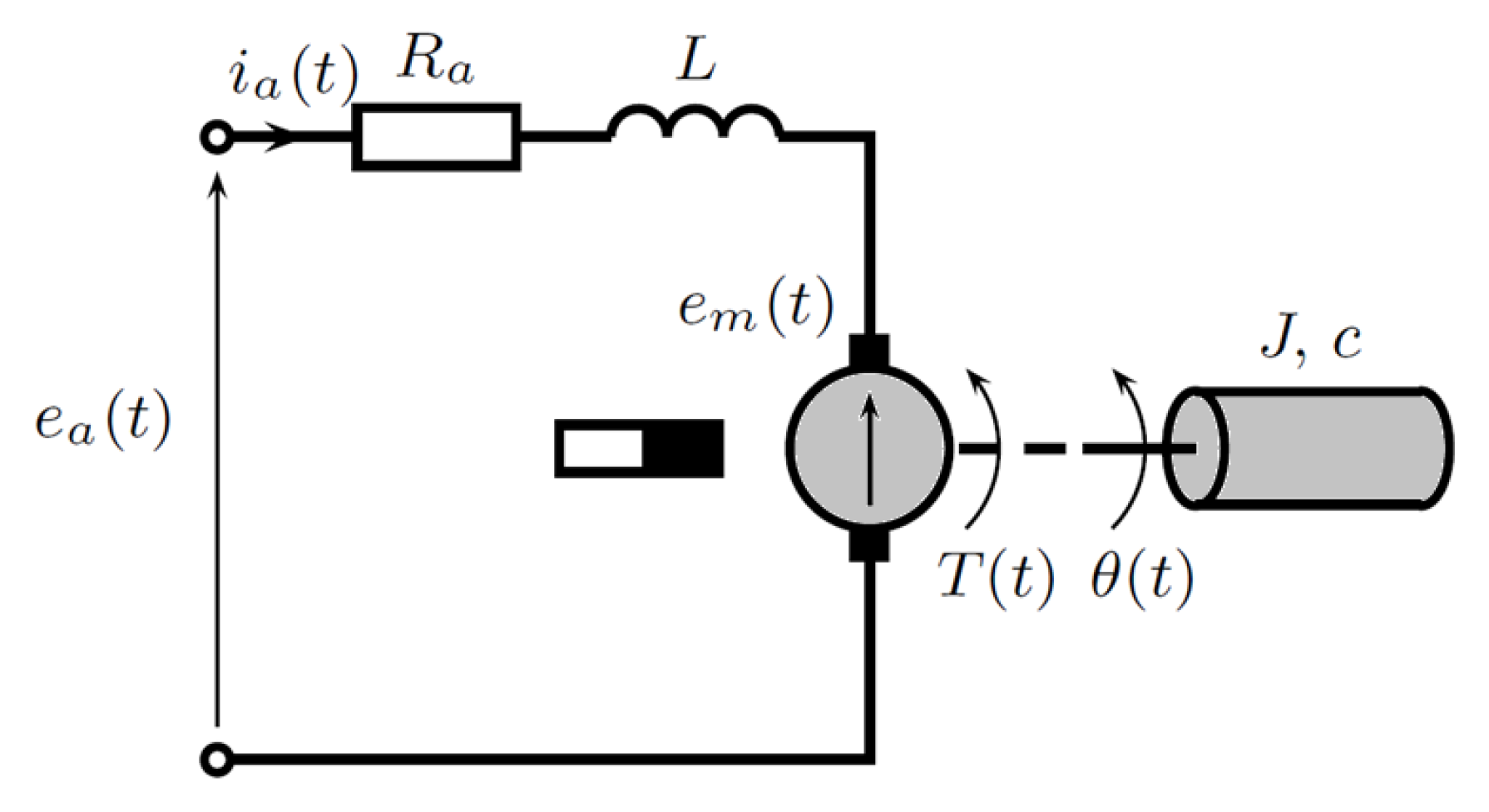
The considered experimental setup consists of a DC Buehler motor [5,6,21]: 12 V, 77 W, 250 mNm, speed 3000 rpm, current 4.7 A, the tachogenerator and the inertia load (brass cylinder, 2 kg, diameter 66 mm, length 68 mm), as shown in Figure 1 [22,23]. The DC motor drives the inertia load and tachogenerator, which is connected directly to the DC motor, with voltage proportional to the angular velocity . Additional modules of the laboratory setup include encoder or magnetic brake modules, as well as a backlash module. The encoder is used to obtain information about the rotation position of the shaft, without the need to integrate the velocity signal.
The command input is fed to the servo drive from an input-output card used by Simulink Coder in order to work in a real-time regime. C-MEX S-functions have been used to implement the controller algorithm and estimation scheme, which has been downloaded to the FPGA board. The control armature voltage is limited to , and is presented in the paper in a dimensionless form as , to present the calculated control signals that are subject to cut-off saturation while performing hardware-in-the-loop experiments.
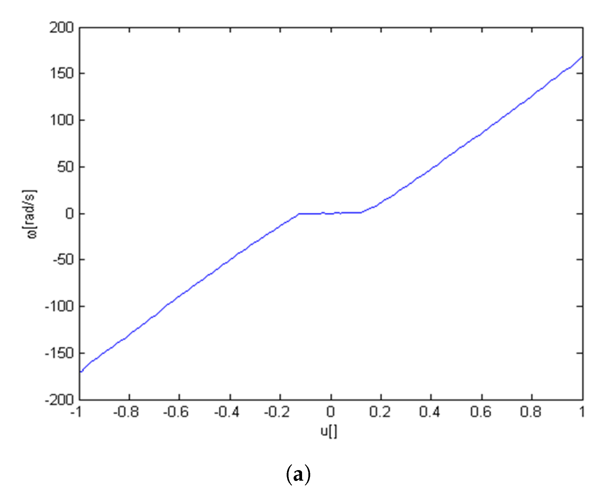
As the nonlinearities present in the considered servo drive include: saturation (of the control signal), dead-zone nonlinearity of a static type as per friction and neglectful mechanical elasticity, one can assume that the control signal can be fed through the inverse static characteristic of the static nonlinearity, leading to linear system equations (when no saturation occurs in dynamic states) [5,21].
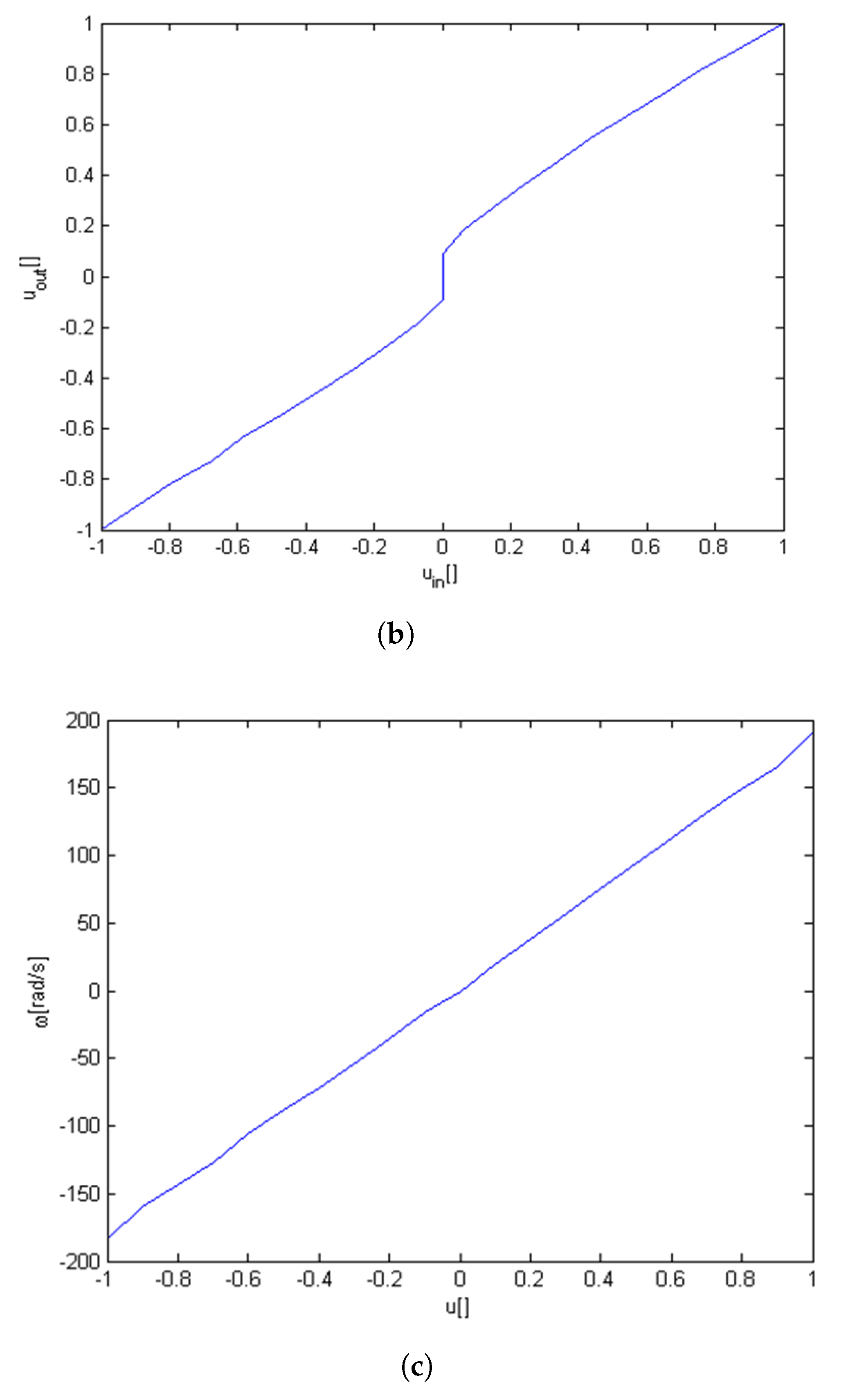
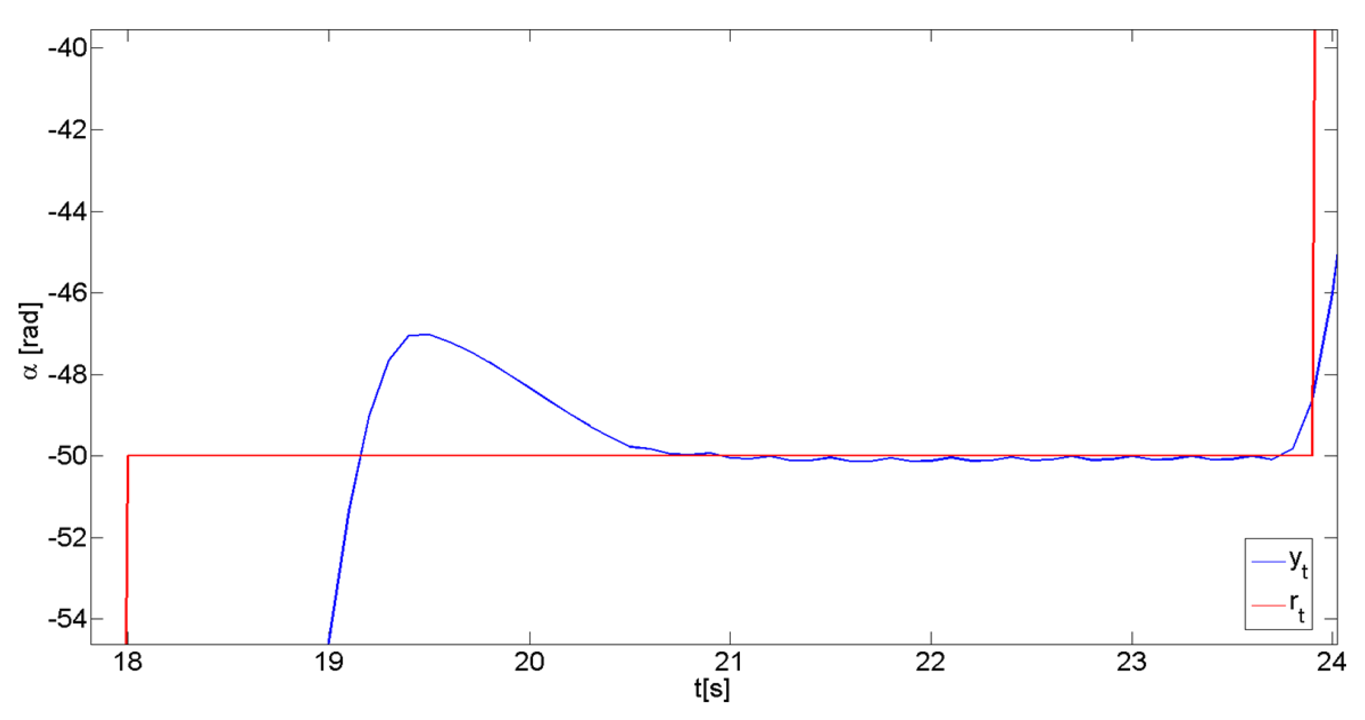
It is to be stressed that when the shaft stabilizes at the position reference value, and the velocity is near zero, the control signal must change rapidly, as the system is insensitive to near-zero signals, which results from the static characteristics presented in Figure 2. These rapid changes in the control signal do not cause sudden changes in the position of the shaft, from the above reasons. A sample illustration is presented in Figure 3.
In accordance with [5], and in the velocity control task, the following formula describes the armature loop on the basis of Kirchoff’s voltage law:
Having assumed that we have a constant flux and electromagnetic force proportional to the rotational speed , as well as the electromechanical torque proportional to the armature current, one gets on the basis of the d’Alembert law of forces
Now, neglecting the armature inductance, the ideal continuous-time model transfer function becomes
with:
As can be seen, the model is very simple, though still accurate [21], enabling good control performance on its basis. The simplicity of the model will streamline the derivation of the analytical form of the predictive control law, and makes this control scheme applicable in a real-time environment, even on systems with low computational power, by omitting the stage of the Diophantine equations solution.
Obviously, velocity- and position-control models differ only by the integration operation, which is standardly performed in the GPC framework at the output of the velocity controller, and represented as the sum operator. However, when the integration operation in the model is taken into account, the sum operator becomes necessary, and the same control law, as derived in the case of velocity control [5,6], can be used here for position control. At the same time, its derivation is the same as in the latter references.
It is assumed that the ZOH-discretized model of this plant is taken into consideration when implementing the GPC algorithm with the sampling period of T = 0.1 s, with voltage input and velocity output, and with the sum operator at the output exchanged for interior integration property, with the encoder output fed back to the controller.
In addition, to justify the selection of a simple model, a series of experimental campaigns has been set to apply the Akaike Information Criterion, which for ARMAX-type models and polynomials describing the model with (9) is defined by
where N is the number of samples, is the variance of residuals (prediction errors), calculated for the parameter estimates of the n-order model,
where:
abiding standard notation from the field of identification.
Having performed a series of experiments in a position control task (input u—voltage, output y—rotation angle of the shaft) with , initial estimates in RLS scheme close to 0, unity forgetting factor and the initial value of a diagonal covariance matrix set at 100 times the unity matrix, the results from Table 1 have been obtained.
The best estimate of the order of the plant has been taken as (voltage input vs. rotational angle output).
When one is interested in the rotational speed control task, the model becomes a simple, first-order inertia, with its ideal values at
identified by an RLS algorithm in a long horizon [24].
In order to streamline the reading of the paper, the notation used in the paper has been summarized in Table 2.
3. Plant Model in the Position Control Task
After linearization of the static characteristics of the plant, and with a measurement noise corrupting the output of the closed-loop system, the model of the plant takes the form [5]:
where and are input and output signal samples, respectively, is assumed to be a white noise with zero mean value and d is a dead time. The introduced polynomials are given as:
Citing after [5], tracking of a reference signal known samples in advance is ensured by the use of the GPC scheme [2,13], where the controller computes consecutive control signals to minimize the following performance index:
where: is an optimal i-step output prediction, is a control signal weight, and are control and prediction horizons, respectively. The weight can severely modify the performance of the closed-loop system, as its improper choice might result in resaturations of control signal or rapid control actions to be taken.
Abiding a standard procedure, by solving a pair of the following Diophantine equations [2]:
where i denotes the output prediction step, the following polynomials can be used ():
Having introduced the above polynomials, step output prediction can be calculated as a sum of forced and free responses:
where:
- is the output prediction, is an impulse response matrix, i.e.,with entries from ,
- is a calculated control signal vector,
- is a free response vector.
In the case of no constraints imposed on the control signal, and for (13), an explicit formula for the control signal can be given as:
As already presented, the Inteco Modular Servo System drive can be modeled as the first-order inertia in the velocity control task, and its discrete-time model is given with , , , i.e.,
and in the case of the position tracking task, the control signal changes (21) are fed to the plant, which integrates them, and as a result, reacts similarly to the model taken in velocity control [6].
An exemplary form of prediction (20) can be presented, say, in two steps ahead (a general rule can be observed from the structure of this prediction) on the basis of the Diophantine equations:
which streamlines generation of control signals according to (21). Furthermore, , , , for example, the measurement noise is identified to be of a white noise type, which in general is a practical case.
The details of implementation in C code are given in [5], and results of actuator/sensor failure behaviour of the system in the velocity control task are given in [6]. These follow the same analysis method and can be similarly presented in a graphical way as in the paper. As already stated, this paper aims at extending the results to the position control task, with the solution of a set of Diophantine equations obtained without solving any matrix inverse problems and simply by observing the relations in (23), which substantially streamlines the implementation of the controller.
The predictive controller has been implemented as a C-MEX S-function, using standard C commands, dynamic tables, and a Lapack library to enable matrix operations. The S-function framework admitted to splitting the code into identifiable routines related to the updates of the internal states of the controller (its memory between the consecutive sampling periods), updates at its output, and current operations performed at every sampling period. Similarly, the identification routine has been implemented as a C-MEX S-function, with its internal states connected to the covariance matrix, as well as to prior estimates. The identification routine has been fed with samples of the output and the constrained input of the plant, and triggered every sampling period to update estimates, as in Figure 4. The complete listings in C can be obtained from [5].
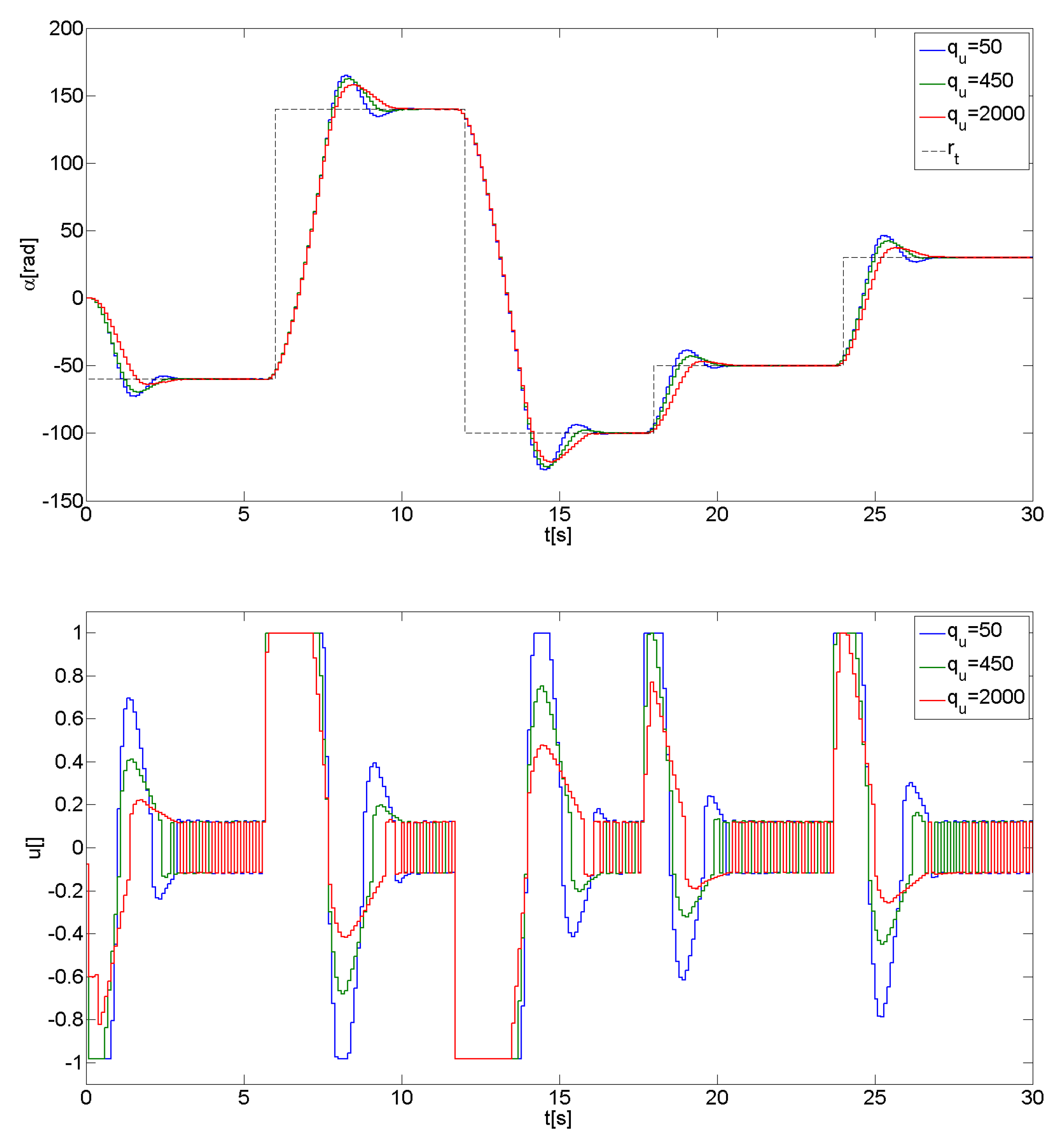
A good choice of the control effort weight results in high performance of the control system. On the basis of initial simulations based on an identified model in the fault-free case, for a set of weighing factors, it has been observed that an increase in above 450 resulted in a decrease in control signal values, limited here to one. Further increase above decreased jerks in the output signals, as well as smoothed the control signal, see Figure 5. Finally, this parameter has been set at . Both control re-saturation as well as tracking issues need to be tacked out by a proper choice of the latter parameter.
The next sections present experimental results obtained from the laboratory stand with a sampling period of .
4. Considered Schemes of Actuator or Sensor Failures
Classical controllers tolerate failures of actuators or sensors to a limited extent. In actual implementations, the actuators may be subjected to all types of failures of one form or the other, thus it is of practical interest to identify the configuration of a controller that might be called reliable. For reliable controller design there are multiple methods to include sensor or actuator failure information into the closed-loop system design process to ensure robust stability or robust performance. Some of the approaches available in the literature usually treat this problem as the control outage problem, not as a partial failure issue. This could be, furthermore, related to sensor failure issues. As in the case of the velocity control task [6], all the reported experimental results have been carried out in a fully adaptive system using the on-line RLS identification scheme of the model of the plant in the control system, with the initial estimates equal to half of their true values. The ’true’ estimates of the plant parameters have been identified prior, in a long time horizon for sufficiently exciting input signal and forgetting factor equal to unity [1]. The presented results are connected to changes in classical performance indices, such as integral of the absolute error (IAE) and integral of the squared error (ISE) calculated on the basis of continuous-time signals from the tracking system, in the whole experiment horizon. The following formulae provide the values of performance indices with e as the tracking error:
where denotes a time instant, and t defines the time instant related to the moment of observation, usually equal to the duration of a single experiment.
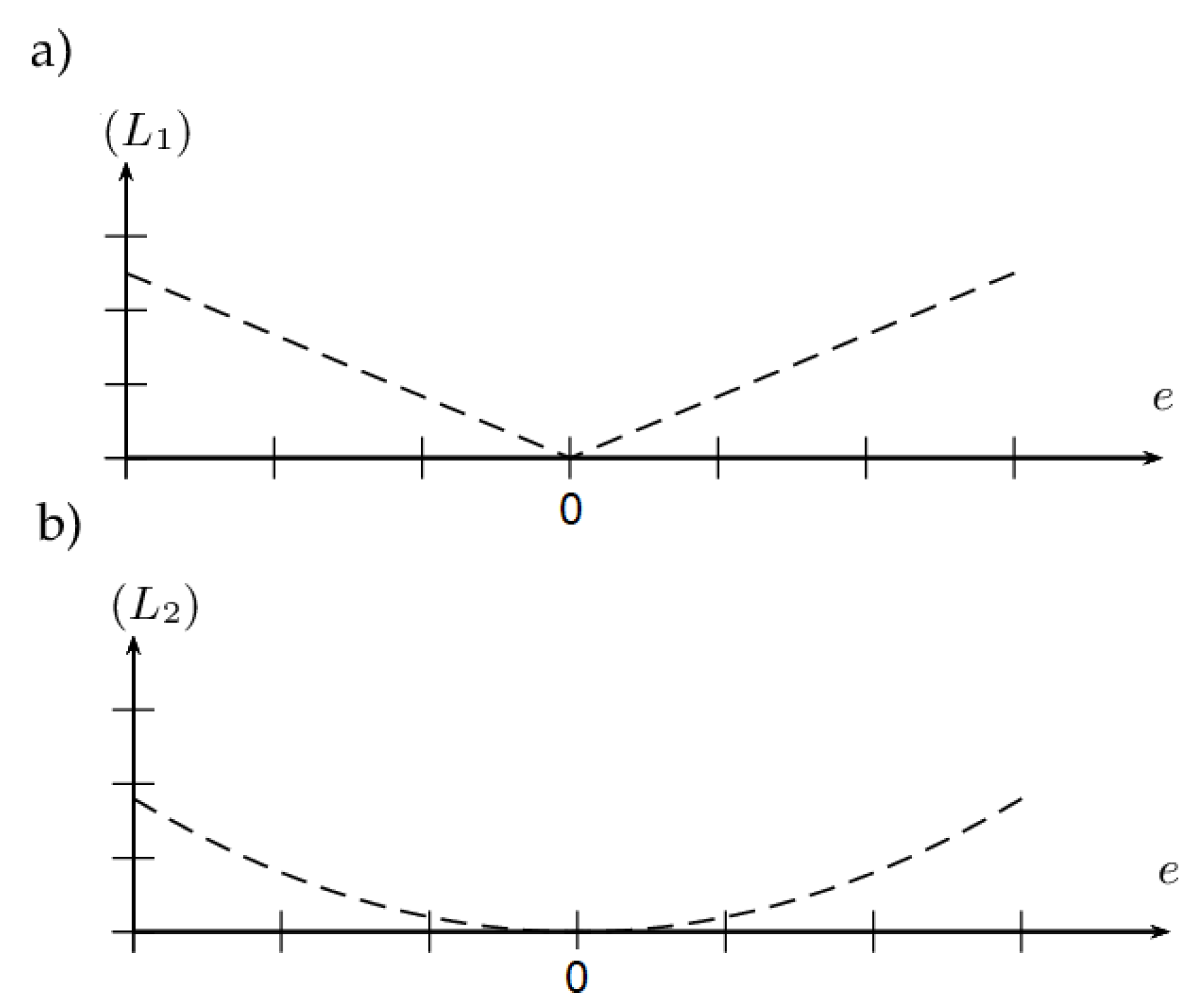
Sub-performance index expressions are related to and penalties imposed on the error, which could be visualized in the form of the penalty function plot, as in Figure 6. The larger the value of the error, with respect to its zero value when the penalty reaches its minimum, the greater the impact of the error on the overall value of a performance index. In the case of IAE, the errors cause linear increase with respect to the increase in the amplitudes of errors, whereas in the case of ISE, the larger errors cause a more severe penalty, and near-zero errors are almost dismissed.
Every measurement series for a particular failure considered has been carried out as a set of individual 55 experiments (all allowable configurations), repeated four times, with mean values presented, to diminish the impact of possible outliers.
When considering the robustness of the GPC control scheme of this plant in unmodelled situations, as in [6], the below-listed cases have been considered:
- Tachogenerator failure (mechanical backlash module between brass cylinder and encoder),
- Actuator failure (mechanical backlash module between DC motor and brass cylinder),
- Break failure (magnetic brake module included in the system).
The performance indices have been depicted as differences between the case with the selected failure model and the nominal case with no failure (for a particular choice of configuration of the prediction horizons, and averaged over four trials to diminish the impact of possible erroneous measurements on their values), both in the sense of absolute value change and relative (i.e., percentage) change—positive values refer to performance deterioration, i.e., increase in performance indexes, and negative—improvement. The values have been presented as colors depicted in triangular areas as per above-mentioned allowable prediction horizon configurations. Obviously the values of indices vary between the sub-figures, as a function of the norm, which forms a sub-integral term. Since the choice of configuration parameters is done over a discrete set of values, the neighbouring points may have different values related to the performance indices’ values. One should interpret the values not on the basis of a single configuration, but rather on the basis of a tendency in an area. This is the same as with the short-sightedness phenomenon widely discussed in the conditioning technique approach to anti-windup compensation in the case of input constraints, which might be somewhat related to desaturation properties of the control signal by a proper choice of horizons in predictive control or the weight.
5. Sensor Failure Case
Sensor faults may appear and evolve in a variety of forms, impeding the way the faults are represented for control and estimation purposes. As in the case of a general identification problem, the faults may be represented by a parametric or a nonparametric approach, and may be included in the synthesis stage. Parametric representations of the faults often result in models of plants that are affine in parameters to pursue with recursive identification schemes. On the other hand, one could simply verify the ability of the adopted control scheme to cope with sensor faults, for different configurations of controller parameters.
When the mechanical backlash unit is connected in series with the DC motor, and precedes the brass cylinder module and the encoder, the sensor failure case is modelled. For such a case, changes of the signals in dynamic states are generated by the encoder only after a full rotation of the shaft is made, making the tracking system insensitive to a position translation smaller than one rotation. With such a configuration of the system, four series of measurements have been carried out, in analogy to the series presented in [5].
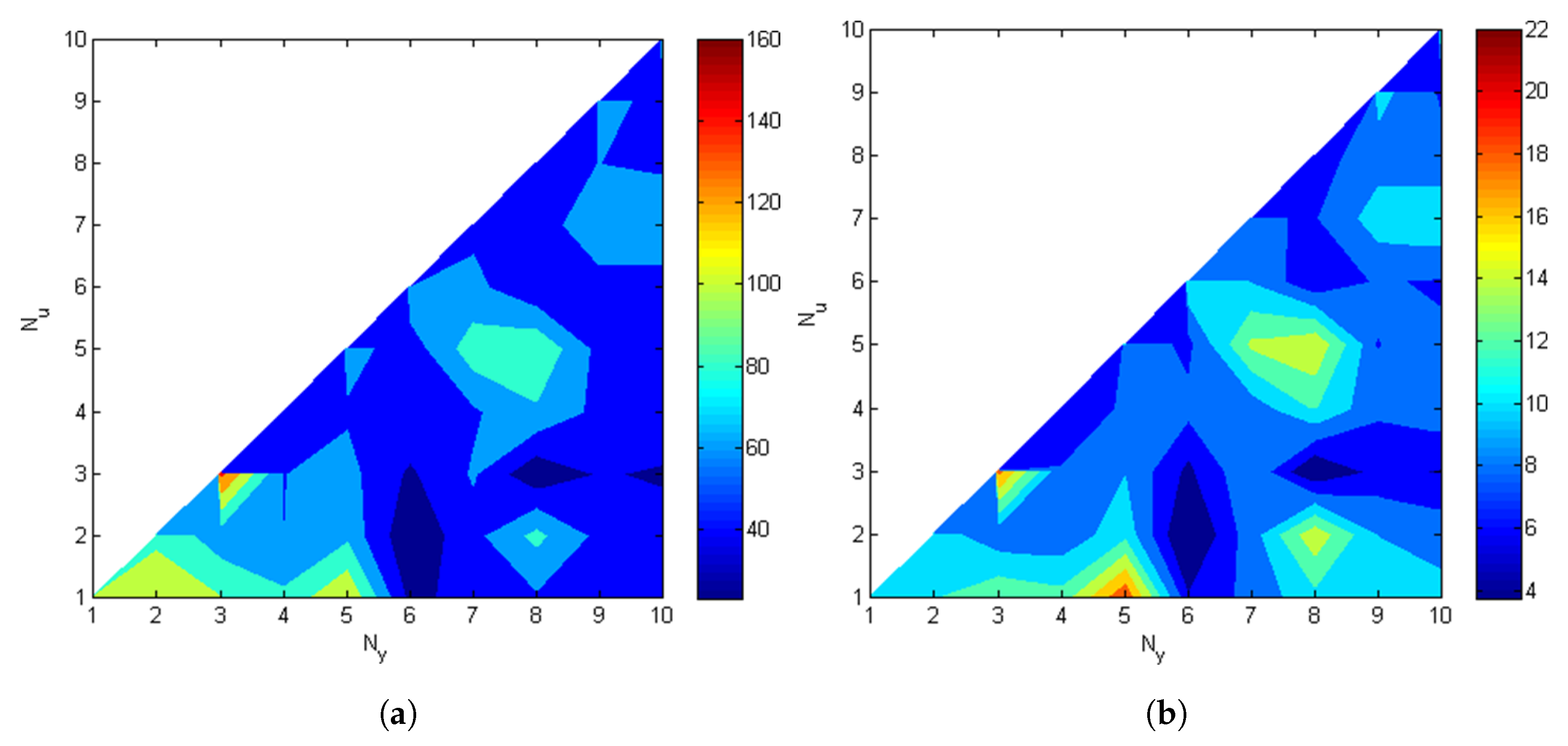
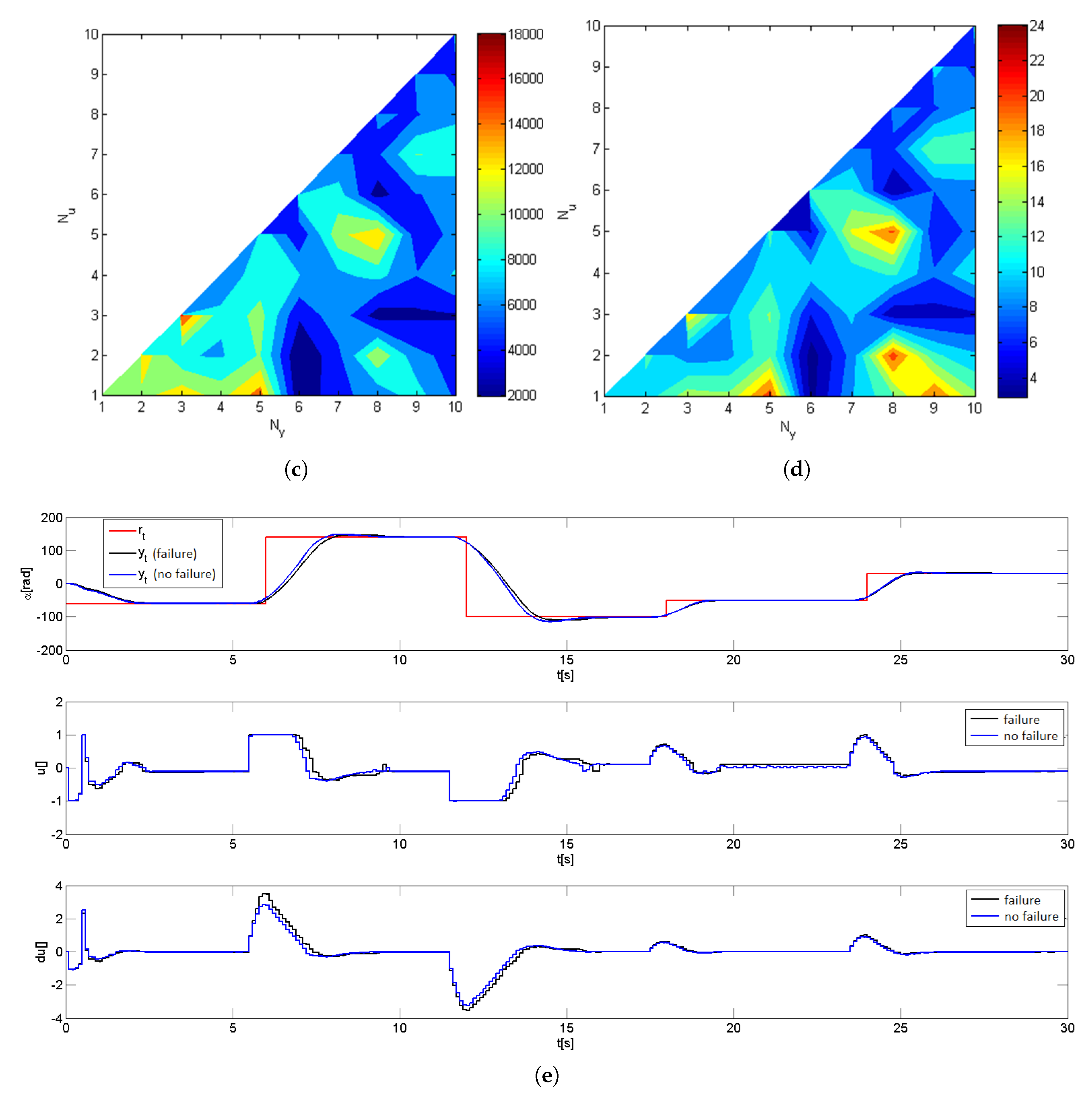
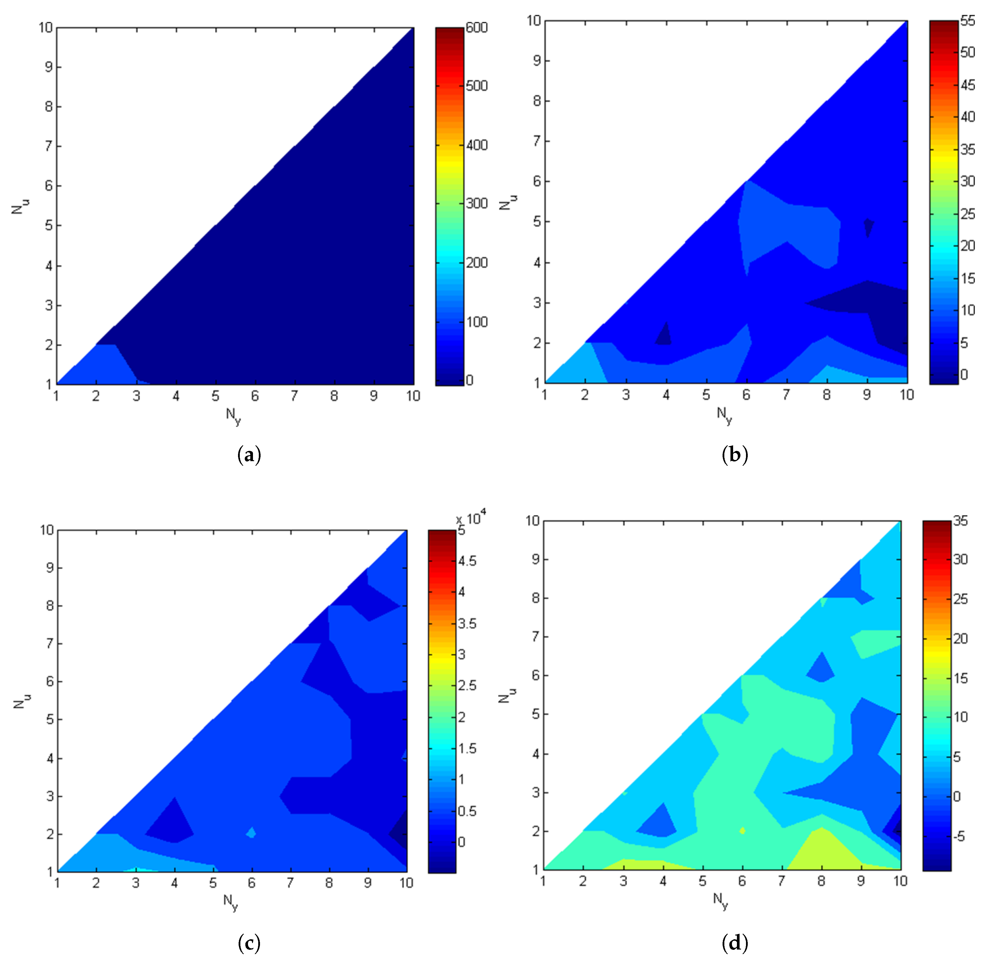
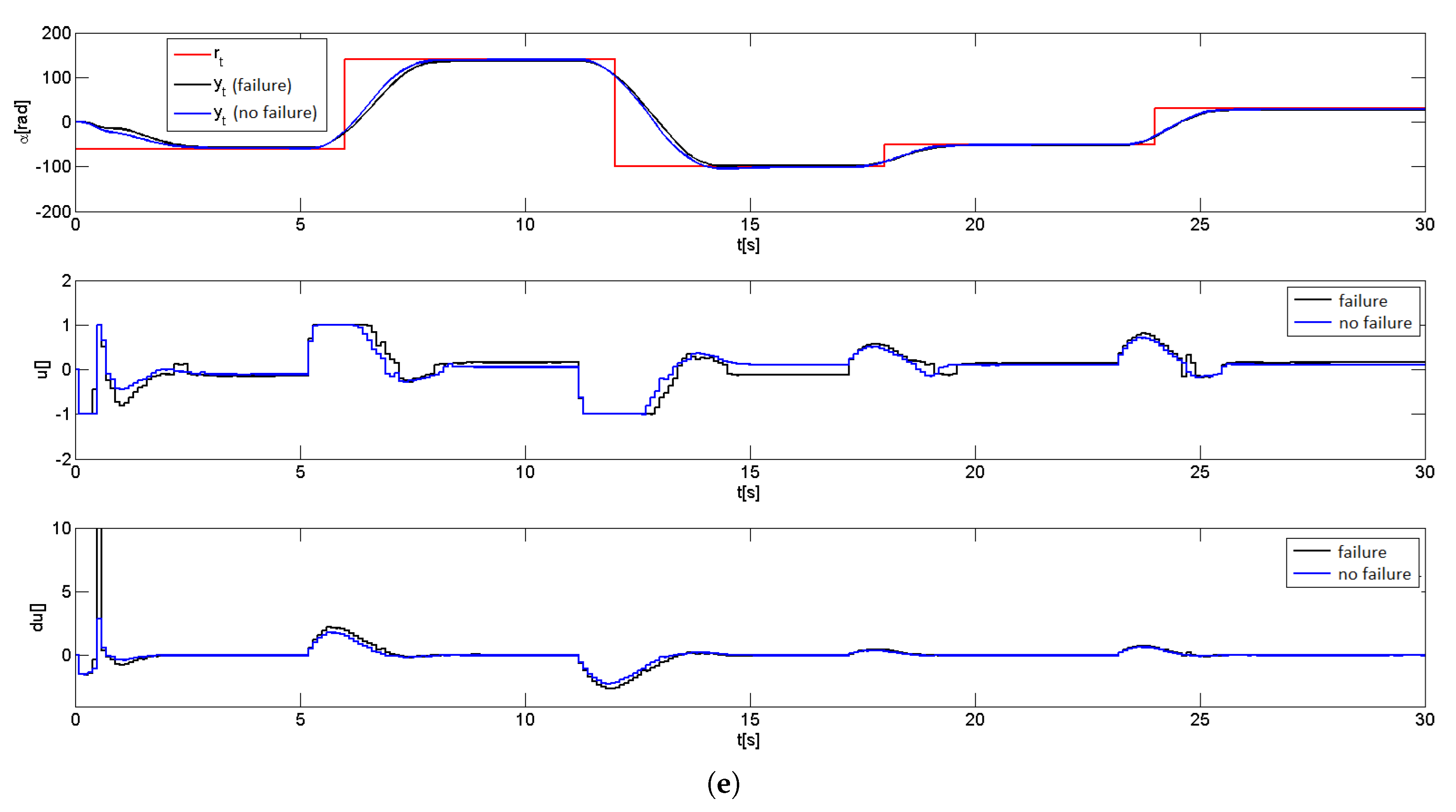
As stated above, the results are averaged over a number of trials. Nevertheless, the results exceeding the doubled mean value of all performance indexes have been additionally cut-off at the level of the mean value. Figure 7a–d presents the cut-off and averaged results. As can be seen in the graphical representation of the results, the introduction of the sensor failure model at gives a drastic performance deterioration, with a 75% increase in ISE, and 95% increase in IAE before the cut-off operation, as reported in classical literature, and related to one-step control. The best absolute and relative results have been achieved when has taken small values and has been at approximately six, i.e., circa a half of T (estimated to be 1.06 s). For this particular configuration, Figure 7e, presents the results of a sample experiment in the situation with and without actuator failure with the same configuration of the controller.
For the failure of this kind, the advantageous policy, ensuring the smallest performance deterioration, is to keep a relatively long and short . In this case, the control signal ensures fast transients, the control action is not extended to a number of future samples, which improves the adaptation process. As in the case of the velocity control [6], larger control signal horizons cause deterioration of the performance during reverse of the shaft.
6. Actuator Failure Case
Robustness of feedback control systems gives rise to an implicit fault tolerance, to some extent. Faults that take place under the closed-loop control are prone to be compensated by the control actions. The same applies when the MPC is used at the control level, and despite the unavailability of the knowledge of the fault, the MPC controller automatically might take advantage of the fault tolerance in this control scheme.
Having connected the mechanical backlash module between the DC motor and the brass cylinder, one can model actuator failure-like behaviour in a repeatable way. The instantaneous change in the rotation angle of the shaft of the motor does not cause an immediate rotation of the brass cylinder. Such a configuration of the experimental setup disables the possibility to track reference signals, again, smaller in amplitude than one rotation of the shaft, since the system has an inherent dead-zone there.
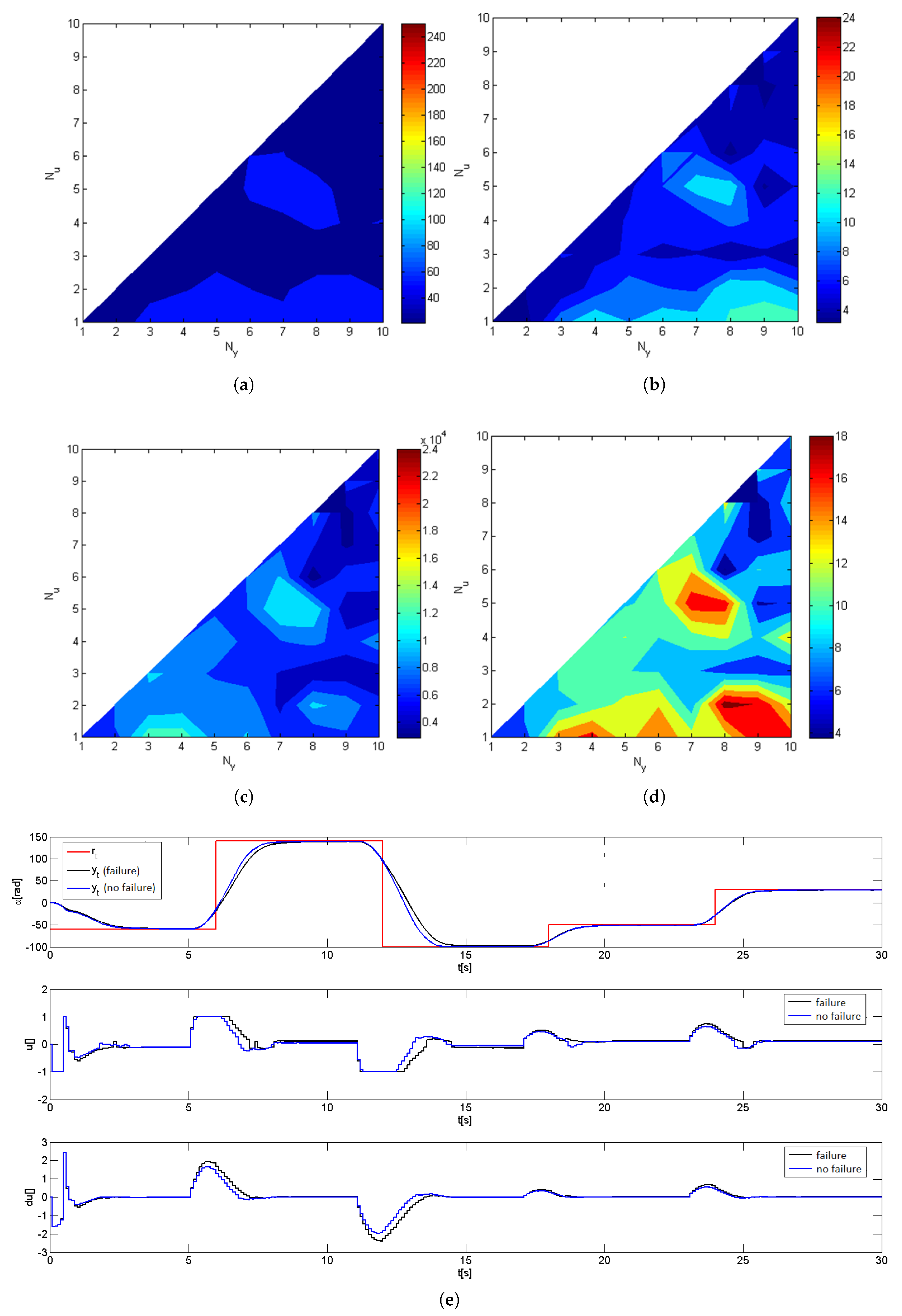
As in the case of sensor failure case, the actuator failures mostly degrades the performance in the case of short control horizons (Figure 8). The proper configuration in this case would be to select large values of and short , for example, the configuration with and , where the performance indexes noted a slight improvement, both in IAE and ISE. The sample result, where a steady-state error of 2 ÷ 3 rad can be observed, is presented in Figure 8e.
The reciprocal situation has been described in [6], where this particular failure had no impact on the steady-state performance, but on increasing the dominating time constant of the closed-loop system, as in this case. In the position control task, when failure occurs, the shaft rotates slower, leading to longer saturation period in the control signal, making adaptation conditions worse.
7. Brake Failure Case
To perform this stage of experiments, the laboratory stand has been modified and required the installation of the magnetic brake unit between the brass cylinder and the encoder. Along the rotation of the shaft, due to Faraday’s law of induction, the current is induced in which magnetic fields generate the load torque, according to Lenz’s law, in the form of a step change, kept until the end of the experiment. In this part of the experiment, two measuring series have been performed, each composed of 55 simple measurements (see Figure 9).
The worst performance degradation, as in the case of prior experiments concerning two failure modes, leading to 25% deterioration in IAE and 19% deterioration in ISE indices, is observed for (the cut-off level for the outliers has been chosen previously). Good results have been obtained for the configurations with large , and the smallest impact of brake failure on the performance of the system has been observed for , and , . A sample result of the experiment has been presented in Figure 9e.
In contrast to the velocity control, brake failure (i.e., introduction of braking past some failure) results in changes with the control signal and affects the dynamics of the closed-loop system, as the dominating time constant increases (not visible from formulas describing the model, as this phenomenon is not taken into account there). In the case of the velocity control task from [6], it has even been possible to improve the control performance, which is not visible in the current research. The translation from one angle to the other takes simply more time.
8. Summary and Conclusions
Figure 10 presents three selected configurations depicting the tracking performance as the function of the IAE performance index value. In the case of low-IAE value, control rate change is at its lowest, giving rise to poor excitation conditions of the identification algorithm. On the contrary, when the controller’s parameter combination is selected to obtain a high value of the IAE index, the system is more dynamic, the control signal changes abruptly, causing faster adaptation of the estimates of the parameters of the plant to their true values. This factor must also be taken into account in all the three selected failure modes in the adaptive control system.
A situation of failures of the control system and their impact on predictive controller behaviour in such cases, to obtain a reliable control system, where performance degradation is neglectful, and the configurations of prediction horizons ensuring the latter, have been identified and presented in the paper. The author has not found any references in the research as to whether the GPC scheme can tolerate any failures either in the actuator or sensor, which has given rise to this research concerning position control. Such an analysis might be of practical interest, especially when the results are obtained from real-world hardware.
In the case of the considered sensor failure, the predictive scheme ensured retaining the best control performance for short control horizon, and long prediction horizon, as the predicted response samples (forced and free) enabled one to improve control performance by observing an eventual increase in the cost function. Similar conclusions hold in the case of actuator failure, this time enabling slight improvement in control performance. This can be thought of as the result of long-horizon planning for a large horizon. In order to minimize the effects of accidental break failure, the control horizon needs to be increased to compensate for the need to exert greater/longer control actions.
It is to be added that on the contrary to the case of the velocity control task, in position control, the linearization, which has obviously been imprecise, caused small steady-state errors to appear with amplitudes 0.5 ÷ 1 rad, which are neglectful here.
Funding
This research was funded by the Poznan University of Technology grant number 0214/SBAD/0220, and the APC was funded by Poznan University of Technology.
Institutional Review Board Statement
Not applicable.
Informed Consent Statement
Not applicable.
Data Availability Statement
Not applicable.
Acknowledgments
The author wishes to express his gratitude to Pawel Szczygiel for invaluable help in conducting experiments for this paper.
Conflicts of Interest
The author declares no conflict of interest.
References
- Åström, K.J.; Wittenmark, B. Adaptive Control; Addison-Wesley: Boston, MA, USA, 1989. [Google Scholar]
- Camacho, E.; Bordons, C. Model Predictive Control; Springer: London, UK, 1998. [Google Scholar]
- Zietkiewicz, J.; Kozierski, P.; Giernacki, W. Particle swarm optimisation in nonlinear model predictive control; comprehensive simulation study for two selected problems. Int. J. Control 2020, 1–17. [Google Scholar] [CrossRef]
- The Mathworks. Real-Time Workshop. User’s Guide. 2015. Available online: https://edulab.unitn.it/nfs/Manualistica/Software/MathWorksGuide/rtw/rtw_gs.pdf (accessed on 19 February 2021).
- Horla, D. C-code implementation of an adaptive real-time GPC velocity controller for a servo drive. In Proceedings of the 17th International Conference on Mechatronics, Prague, Czechia, 7–9 December 2016; pp. 1–6. [Google Scholar]
- Horla, D. Adaptive predictive controller for a servo drive – actuator/sensor failure study experiments. In Proceedings of the 14th International Conference on Informatics in Control, Automation and Robotics, Madrid, Spain, 26–28 July 2017; pp. 551–558. [Google Scholar]
- Yang, G.-H.; Wang, J.L.; Soh, Y.C. Reliable LQG control with sensor failures. IEE Proc. Control Theory Appl. 2000, 147, 433–439. [Google Scholar] [CrossRef]
- Yang, Y.; Yang, G.-H.; Soh, Y.C. Reliable control of discrete-time systems with actuator failures. IEE Proc. Control Theory Appl. 2000, 147, 428–432. [Google Scholar] [CrossRef]
- Zuo, Z.; Ho, D.W.C.; Wang, Y. Fault tolerant control for singular systems with actuator saturation and nonlinear perturbation. Automatica 2010, 46, 569–576. [Google Scholar] [CrossRef]
- Mhaskar, P.; Gani, A.; Christofides, P.D. Fault-tolerant control of nonlinear processes: Performance-based reconfiguration and robustness. In Proceedings of the American Control Conference, Minneapolis, MN, USA, 14–16 June 2006. [Google Scholar]
- Knudsen, B.R.; Faulwasser, T.; Jones, C.N.; Foss, B. Incipient Actuator Fault Handling Nonlinear Model Predictive Control. IFAC-PapersOnLine 2017, 50, 15922–15927. [Google Scholar] [CrossRef]
- Bavili, R.E.; Khosrowjerdi, M.J.; Vatankhah, R. Active Fault Tolerant Controller Design using Model Predictive Control. J. Control Eng. Appl. Inform. 2015, 17, 68–76. [Google Scholar]
- Maciejowski, J. Predictive Control with Constraints; Pearson: London, UK, 2001. [Google Scholar]
- Xu, F.; Puig, V.; Ocampo-Martinez, C.; Olaru, S.; Niculescu, S.-I. Robust MPC for Actuator-fault Tolerance using Set-based Passive Fault Detection and Active Fault Isolation. Int. J. Appl. Math. Comput. Sci. 2017, 27, 43–61. [Google Scholar] [CrossRef] [Green Version]
- Ocampo-Martinez, C.; Guerra, P.; Puig, V.; Quevedo, J. Actuator Fault-tolerance Evaluation of Linear Constrained Model Predictive Control using Zonotope-based Set Computations. J. Syst. Control Eng. 2007, 221, 915–926. [Google Scholar] [CrossRef]
- Nebeluk, R.; Ławryńczuk, M. Tuning of Multivariable Model Predictive Control for Industrial Tasks. Algorithms 2021, 14, 10. [Google Scholar] [CrossRef]
- Shiquan, Z.; Anca, M.; Sheng, L.; De Keyse, R.; Ionescu, C. Effect of Control Horizon in Model Predictive Control for Steam/Water Loop in Large-Scale Ships. Processes 2018, 6, 265. [Google Scholar]
- Ionescu, C.; Copot, D. Hands-on MPC tuning for industrial applications, Bulletin of the Polish academy of sciences. Tech. Sci. 2019, 67, 925–945. [Google Scholar]
- Horla, D.; Sadalla, T. Optimal tuning of fractional-order controllers based on Fibonacci-search method. ISA Trans. 2020, 104, 287–298. [Google Scholar] [CrossRef] [PubMed]
- Horla, D. Robust performance of sampled-data adaptive control of a servo drive. From simulation to experimental results. J. Autom. Mob. Robot. Intell. Syst. 2015, 9, 3–8. [Google Scholar]
- Horla, D. Minimum variance adaptive control of a servo drive with unknown structure and parameters. Asian J. Control 2013, 15, 120–131. [Google Scholar] [CrossRef]
- Inteco. Modular Servo System USB Version Installation Manual; 2015; Available online: http://www.inteco.com.pl/user-support/ (accessed on 19 February 2021).
- Inteco. Modular Servo System User’s Manual; 2015; Available online: https://www.a-lab.ee/man/Servo-user-manual.pdf (accessed on 19 February 2021).
- Ljung, L. Recursive Identification Algorithms; Technical Report; Linköping University: Linköping, Sweden, 2000. [Google Scholar]
Figure 1.
Diagram of the experimental setup.

Figure 2.
Linearization of the static characteristics of the plant. (a) Static characteristic of a servo drive; (b) Static characteristic of the compensator; (c) Final static characteristic of the linearized plant.
Figure 2.
Linearization of the static characteristics of the plant. (a) Static characteristic of a servo drive; (b) Static characteristic of the compensator; (c) Final static characteristic of the linearized plant.


Figure 3.
Position tracking with , , s.

Figure 4.
Setup to obtain values of AIC.

Figure 5.
A proper choice of for , .

Figure 6.
Penalty function plots vs. error, (a) , (b) penalty functions.

Figure 7.
Experimental results concerning sensor failure with , s. (a) Absolute IAE change; (b) Relative IAE change; (c) Absolute ISE change; (d) Relative ISE change; (e) Tracking performance with and without sensor failure, , .
Figure 7.
Experimental results concerning sensor failure with , s. (a) Absolute IAE change; (b) Relative IAE change; (c) Absolute ISE change; (d) Relative ISE change; (e) Tracking performance with and without sensor failure, , .


Figure 8.
Experimental results concerning actuator failure with , s. (a) Absolute IAE change; (b) Relative IAE change; (c) Absolute ISE change; (d) Relative ISE change; (e) Tracking performance with and without actuator failure, , .
Figure 8.
Experimental results concerning actuator failure with , s. (a) Absolute IAE change; (b) Relative IAE change; (c) Absolute ISE change; (d) Relative ISE change; (e) Tracking performance with and without actuator failure, , .


Figure 9.
Experimental results concerning brake failure with , s. (a) Absolute IAE change; (b) Relative IAE change; (c) Absolute ISE change; (d) Relative ISE change; (e) Tracking performance with and without brake failure, , .
Figure 9.
Experimental results concerning brake failure with , s. (a) Absolute IAE change; (b) Relative IAE change; (c) Absolute ISE change; (d) Relative ISE change; (e) Tracking performance with and without brake failure, , .

Figure 10.
Selected experiments on the basis of integral of the absolute error (IAE) values, with , s.
Figure 10.
Selected experiments on the basis of integral of the absolute error (IAE) values, with , s.


Table 1.
AIC criterion values for .
| n | 1 | 2 | 3 | 4 | 5 |
|---|---|---|---|---|---|
| AIC(n) |
Table 2.
Notation used throughout the paper.
| Symbol | Meaning |
|---|---|
| y | output signal (rotation angle of the shaft) |
| rotational velocity of the shaft | |
| v | calculated control signal |
| u | applied/constrained control signal |
| r | reference signal |
| disturbance signal affecting model’s output | |
| q | time-shift operator (discrete-time domain) |
| sampling period | |
| , | control and output prediction horizons |
Publisher’s Note: MDPI stays neutral with regard to jurisdictional claims in published maps and institutional affiliations. |
© 2021 by the author. Licensee MDPI, Basel, Switzerland. This article is an open access article distributed under the terms and conditions of the Creative Commons Attribution (CC BY) license (http://creativecommons.org/licenses/by/4.0/).
Share and Cite
MDPI and ACS Style
Horla, D. Experimental Results on Actuator/Sensor Failures in Adaptive GPC Position Control. Actuators 2021, 10, 43. https://0-doi-org.brum.beds.ac.uk/10.3390/act10030043
AMA Style
Horla D. Experimental Results on Actuator/Sensor Failures in Adaptive GPC Position Control. Actuators. 2021; 10(3):43. https://0-doi-org.brum.beds.ac.uk/10.3390/act10030043
Chicago/Turabian StyleHorla, Dariusz. 2021. "Experimental Results on Actuator/Sensor Failures in Adaptive GPC Position Control" Actuators 10, no. 3: 43. https://0-doi-org.brum.beds.ac.uk/10.3390/act10030043
Note that from the first issue of 2016, this journal uses article numbers instead of page numbers. See further details here.