
Tracking Control of Pneumatic Artificial Muscle-Activated Robot Arm Based on Sliding-Mode Control


1
Graduate Institute of Automation Technology, National Taipei University of Technology, Taipei 10608, Taiwan
2
Department of Mechanical Engineering, National Chin-Yi University of Technology, Taichung 41170, Taiwan
3
Department of Mechanical Engineering, National Chung Cheng University, Chiayi 621301, Taiwan
4
Advanced Institute of Manufacturing with High-Tech Innovations, National Chung Cheng University, Chiayi 621301, Taiwan
*
Author to whom correspondence should be addressed.
Actuators 2021, 10(3), 66; https://0-doi-org.brum.beds.ac.uk/10.3390/act10030066
Submission received: 3 February 2021
/
Revised: 18 March 2021
/
Accepted: 19 March 2021
/
Published: 22 March 2021
(This article belongs to the Special Issue Actuators in Robotic Control)
Abstract
:This study discusses a circular trajectory tracking function through a proposed pneumatic artificial muscle (PAM)-actuated robot manipulator. First, a dynamic model between a robot arm and a PAM cylinder is introduced. Then the parameters thereof are identified through a genetic algorithm (GA). Finally, PID is used along with a high-order sliding-mode feedback controller to perform circular trajectory tracking. As the experimental results show, the parameters of sampling time and moment of inertia are set to accomplish the trajectory tracking task in this study. In addition, the maximum error between the objective locus and the following locus was 11.3035 mm when applying theta-axis control to the circular trajectory of the robot arm with zero load or lower load. In an experiment of controller comparison, the results demonstrate that a high-order sliding-mode feedback controller is more robust in resisting external interference and the uncertainty of modeling, making the robot arm have good performance when tracking.
1. Introduction
In recent years, with the rise of interdisciplinary concepts and the trend toward mechanical automation, automated robots have gradually begun to stand out in various industrial markets, such as service and medical treatment. Especially in the field of biomedicine, improvements in the quality of life and in the aging population have greatly evoked a demand for medical services, and shortage of medical personnel has become a problem that the entire medical industry must confront, where what a physiotherapist does is a labor-intensive job, combined with a frequent occurrence of accidents, sports injuries, and occupational injuries, making rehabilitation robots even more valuable [1,2]. The movements performed by rehabilitation robots cover all four extremities, and for different types of patients, upper-extremity rehabilitation robots have to perform different rehabilitation tasks. Therefore, numerous upper-extremity rehabilitation robots have been developed in the market to assist physiotherapists in their medical tasks [3,4]. Moreover, the demand for rehabilitation tasks is very high in poststroke patients [5,6]. The robot arm used in this study to carry out rehabilitation is designed for stroke patients. Since there are still many machines using a gear reducer and motor as drivers in the medical field, it is often easy to directly apply force to the patient, causing secondary injuries, where the purpose of the motion trajectory is to implement rehabilitation on the patient’s elbow and shoulder. As a result, the pneumatic artificial muscle (PAM) cylinder flexibility can be used to reduce the risk of injuring users. A PAM cylinder is an air-pressurized actuator, with the McKibben type being one of the most renowned actuators [7,8]. A McKibben-type PAM cylinder has the advantages of light weight, flexibility, and nonlinear passive flexibility compared with other actuators [9]. In recent years, PAMs have been frequently used in research studies related to robots, which include modeling and compensation [10,11,12,13,14,15] and control methods [16,17,18]. PAM cylinders have been commercialized by the JSR Corporation and are mainly used for robotics-related applications. McKibben-type PAM cylinders have rubber hoses on the inside and are covered with a fabric mesh on the outside. When the internal rubber hose is pressurized, the pressure inside pushes the hose wall, and the rubber hose is thereby shortened; the contractile force generated is the power source of the actuator’ pneumatic energy. A delay always occurs when a muscle cylinder is repeatedly acting. Minh et al. [19] used proportional flow control servo valves to control PAM cylinders, mainly by experimentally establishing equal-distance, equal-pressure, and equal-delay models, feedforward, and compensation, with good control results. Loukianov et al. [20] provide the concept of sliding-mode control (SMC), where the fundamental idea is to force the system to enter a preset stable space, which is called a sliding plane. The system is restrained in the workspace once it enters, and then it slips toward the control target along the sliding plane. Sárosi et al. [21] used a sliding mode for a robotic arm, driven by a pneumatic muscle actuator. Shen [22] utilized the SMC to collocate with the proportional flow control servo valve to control a PAM cylinder, which is mainly purposed to design the SMC plane for the linear motion control of dual PAM cylinders, as well as to calculate the model and controller parameters via the equivalent control law and mode-switching control (MSC), to form a closed-loop system. Furat and Eker [23] used the second-order SMC to improve the system performance, in which the sliding plane is to be collocated with the second-order sliding plane of PID. From the experiment outcomes, it is provided that resistance to uncertainty and interference of this second-order SMC raises significantly compared with that of the first-order SMC and traditional PID controller.
2. Materials and Methods
2.1. Materials and Experimental Setup
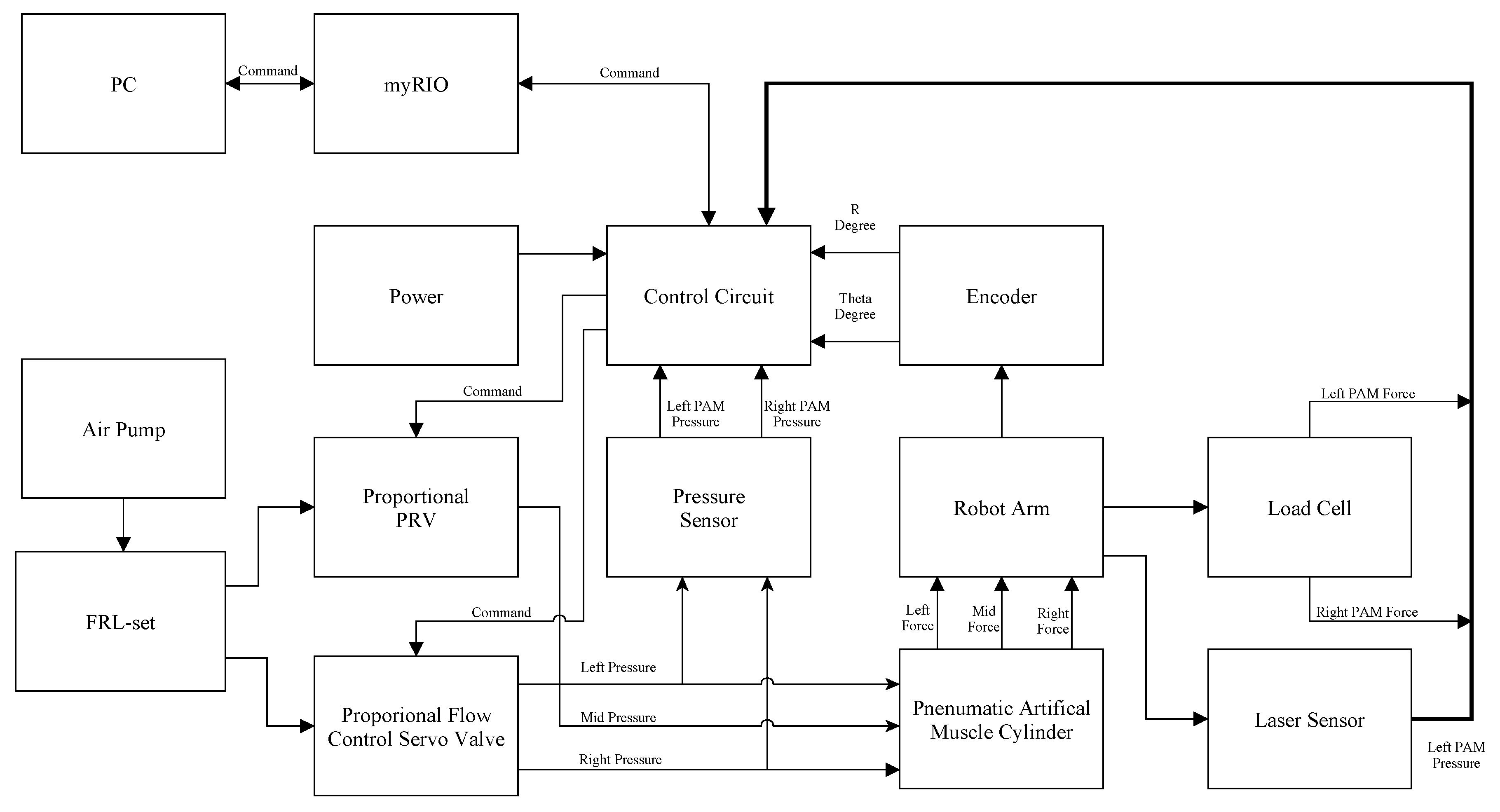
The electromechanical system and structure of the robot arm used in this research is shown in Figure 1: the control terminal consists of a host and a real-time monitoring system, where Windows OS is applied in the host and LabVIEW is used to compile the real-time monitoring program to communicate with the embedded controller. The control flow is that the host delivers the command to the robot arm for the trajectory, and then transfers the data with regard to the trajectory coordinates as well as the correspondent joint angles of the robot arm via forward kinematics to the real-time monitoring system for control. Furthermore, the information feedback by angle, pressure, and force sensor is matched and used to perform tracking. The electromechanical system includes the control system, pneumatic system, robot arm, and detection system. The control system in this study includes the PC, the monitoring and transmission system of the myRIO controller developed by NI, the proportional flow control servo valve (VPPM-6L-L-1-G18-0L10H-V1N) developed by Festo to drive the middle PAM cylinder pulling the R axis as shown in Figure 3, and the proportional flow control servo valve (MPYE-5-M5-010-B) also developed by Festo to drive the two-side PAM cylinders to control the rotation of theta axis. The pneumatic system includes a 3.5 HP air compressor. The robot arm system includes a robot arm with two degrees of freedom and a robot arm joint driven by the PAM cylinder developed by Festo. The motion sketches of the robot arm can be seen in this figure, including the movable joint position, encoder position, and PAM position. The detection system includes an optical rotary encoder, which can detect the angular variation of rotation of each joint of the robot arm; the S-type tension force sensor to measure the force of the PAM applied to the joint; the precision laser rangefinder developed by Keyence to measure the length of the PAM cylinder; and the pressure gauge developed by Festo to measure the inner pressure of the PAM cylinder (SPAB-P10R-G18-NB-K1). In addition, the specifications of other hardware and equipment are shown in Table 1.
2.2. Introduction of a Dynamic Model
2.2.1. Analysis of Motion of Joint Angle and Terminal Point of a Robot Arm System
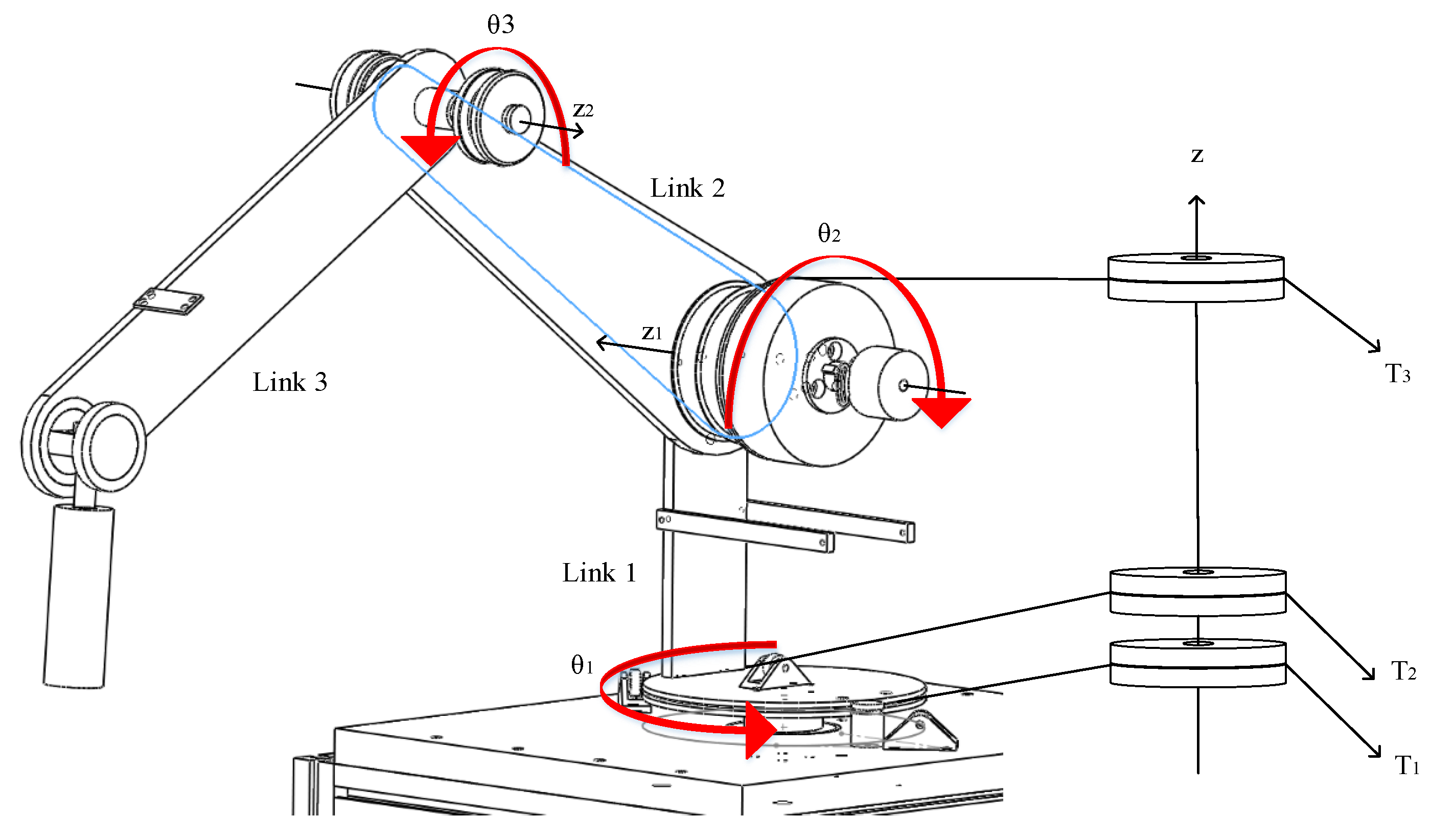
The concept of design of a robot arm in this study mainly aims at executing the planar motion for rehabilitation, in which the robot arm actually consists of three connecting rods. The robot arm has two degrees of freedom because of the mechanism restraint, where the purpose is to generate the motion trajectories on the XY plane of the same Z axis. In order to maintain the end effector of the robot arm to be in motion on the XY plane of the same Z axis, the mechanism design is as shown in Figure 2. The robot arm’s base joint 1 is driven by two sets of artificial muscle cylinders at the same time. When joint 1 rotates, it drives the end effector of the robot arm to rotate at an angle relative to the Z axis. Additionally, to maintain the end effector on the same planar level, the timing belt is used to connect the timing gear 2 of the connecting rod 3 and the timing gear 1 of the connecting rod 2. Due to the connection of the timing belt, the connecting rod 3 simultaneously rotates when the connecting rod 2 is rotary. The rotary angle of joint 1 is defined as , the rotary angle of joint 2 is defined as , and the rotary angle of joint 3 is defined as . Because the gear ratio between joints 2 and joint 3 is two, the angular relation of joints 2 and 3 is as follows:
where the timing gear of joint 2 is brought by an external pulley system, in which the latter is driven by a set of artificial muscle cylinder as shown in Figure 3. Through the design concept of this mechanism, the end effector of the robot arm can be maintained on the same level of the XY plane. Joint 1 is put in motion by the two-sided PAM cylinders pulling a steel rope with each other, while joint 2 is driven by the middle PAM cylinder pulling a steel rope. Joint 1 controls the angle of the end effector of the robot arm projected on a polar coordinate system from the XY plane, while joints 2 and 3 control the radius of the end effector projected on a polar coordinate system from the XY plane. Due to the stroke restraint of an artificial muscle cylinder, the angular range of the end effector rotation is ±15°, while the range of motion of the radius of a polar coordinate system is subject to the range of 10~600 (mm) due to the mechanical restraint.
In this study, we adopt a robot arm with multiple connecting rods, where the base is fixed and the other terminal is so-called the end effector. In order to plan for the trajectory control in the future, kinematics must be used here to define the transforming relationship between two coordinate systems: joint coordination and Cartesian coordination. This study mainly uses the two axial trajectories to track control; therefore, the forward kinematics of the robot arm will be introduced here. The robot arm in this research consists of three connecting rods, where Cartesian coordination is used for the trajectory descriptions in this mission. Considering a robot arm with n degrees of freedom, where the angle is represented as , assuming that the Cartesian coordination of the robot arm is , then the correspondent relationship can be obtained, as in Equation (2).
Denavit and Hartenber (homogeneous transformation matrix, D–H) is used here to define each joint on each coordinate system. Through this methodology, the homologous relationship of the two coordinate systems can be described. Considering the transforming relationship between the positions at and of the two adjacent coordinate systems, there are four important parameters needed when defining the D–H methodology: is the rotary angle of the Z axis corresponding to the previous coordinate system at , is the displacement along the Z axis after the previous coordinate system rotates in the Z axis, is the displacement after the previous coordinate system moves along the Z axis and then the X axis, and is the rotary angle along the X axis after moving along the X axis. After the coordinate transformation of the four coordinates described above, the homogeneous transformation matrix for D–H parameters can be acquired, which is Equation (3):
Relative to the initial position, the correspondent relationship of the robot arm is the function of joint angles, and then the coordinate of the robot arm can be obtained, as in Equation (4).
2.2.2. Dynamic Math and Model of Proportional Flow Control Servo Valve of PAM Cylinder
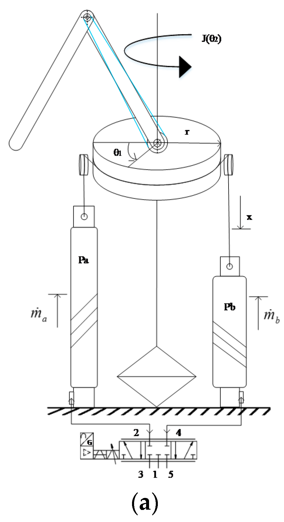
Except for the relativity between the joint angle and the terminal point of the aforementioned robot arm system in Section 2.2.1, the mechanism used in this study also includes the PAM cylinder described in Section 2.2.2. As a result, a model of systematic mathematics is introduced in this section, where the model sketch is shown in Figure 3. It can be divided into three major categories, which include the rotary-load dynamic equation, force dynamic equation, and flow-rate dynamic equation.
In order to prove the rotary-load dynamic equation, this study is referred to the linear MBK system (mass-damper-spring system) to acquire the dynamic, as in Equation (6):
where (kg·mm2) is the moment of inertia of the robot arm; B (kg·mm2/s) is the system damper; is the rotary angular velocity of the robot arm in the theta axis; is the rotary angular acceleration of the robot arm in the theta axis; and (kg·mm/s2) are, respectively, the two forces generated when the PAM cylinder is in motion; and r is the rotary radius of the base axis of the robot arm.
A major power source of the robot arm used in the force dynamic equation is the air pressure inside the hose of the PAM cylinder. Hence, to acquire the force when the two PAM cylinders are activated, the force dynamic equation is required to obtain the pressure–force relationship. This model is represented by the principle of virtual work proposed by Chou and Hannaford, as shown in Equation (7):
where and are the works in regard to input and output, respectively. Therefore, and , where is the force applied by the PAM cylinder; and are the length and volume inside the hose, respectively; is the absolute pressure inside the hose of the PAM cylinder; and is the air pressure of the experiment environment. In order to compute , the fabrics used to cover the PAM cylinder is set to be nonextendable to fix the length thereof, where the volume V of the PAM cylinder is obtained as in Equation (8):
where L is the length of the PAM cylinder (i.e., ), which is the weaving angle of the fabric mesh covering the PAM cylinder; is the diameter of the PAM cylinder (i.e., ); and is the length of fabrics, which is the cycle number of fabrics. Combining Equations (7) and (8), the result is Equation (9):
The relationship when the PAM cylinder is in motion along rotary tools is shown in Equation (10).
is the initial length of the PAM cylinder. Because of , the relationship of the active forces and of the PAM cylinder after combining the equations can be obtained, as in Equation (11):
Use Equations (11) to (6), and then the rotary angle of Equation (12) can be acquired:
Because the proportional flow control servo valve is selected to be the controller in this research, a differential must be performed on the pressure when building the model in order to obtain the first-order differential dynamic equation as in Equation (13):
The pressure variation of the two PAM cylinders can be acquired through differentiation with the ideal gas law, which is shown in Equation (14):
where is the specific heat of air, is the ideal gas constant, is the gas temperature under the experiment environment, and is the variation flow-in/flow-out air mass of the two PAM cylinders. Therefore, the expression of the volume and volume variation of the two PAM cylinders when they are in motion can be proved, as in Equation (15):
Use Equations (14) and (15) into Equation (13), and then we can obtain Equation (16):
where and are the specific kinetic energies of the two PAM cylinders, and is the work applied to joint 1 by the two PAM cylinders.
From the preceding paragraphs, it is shown that the variation rations of air mass and vary along with the opening/closing degree of the proportional flow control servo valve utilized in this study. From the literature [6,7], the formula for the rate of change of air mass is known, so it can be used in Equation (17) to represent the relationship between air flow and valve opening:
where
is the control command of the calculation of the valve opening, and the relationship of the two PAM cylinders is ; and , respectively, represent the upper limit and lower limit of the charged air pressure; is the parameter for the ventilation of the valve opening; and is the parameter used to distinguish the flow-rate formula . Combining the relationships of the control command of the two aforementioned PAM cylinders, and can be concluded, which can be used in Equation (16) to obtain Equation (19):
2.3. Parameter Identification of the Dynamic Model
2.3.1. Parameter Identification of the Model of the Proportional Flow Control Servo Valve
In Section 2.2.2, the model of the proportional flow control servo valve is introduced. In this section, the parameter identification of the model of the proportional flow control servo valve is introduced to achieve the relation in regard to the fundamental open-loop control via control commands and control voltage commands. As a result, the major difference of a proportional flow control servo valve is response speed; by controlling the dimension of the valve opening, the PAM cylinder can be less restrained by the response speed of the hardware when charging or venting. However, the relationship between valve opening and gas flow rate must first be defined before controlling the degree of valve opening. The characteristic graph of the controller used in this study is nonsymmetrical. However, for the convenience and universality of model establishing, the design of the symmetrical relation is used for the control command when defining the flow-rate dynamic equation on valve opening to match this system, that is . Hence, a half-sided characteristic graph is chosen in this study to build the equation of the characteristic curve for curve fitting and the fitting result, whose answer can be proved by reversing the calculation after acquiring the opening percentage of the valve. In order to simplify the calculation of the system, the two relationships are exchanged for refitting, and the relationship is proved. Afterward, the refitting result is used for the information regarding the standard regular flow rate of a proportional flow control servo valve provided by Festo Corporation. Each parameter can be acquired with respect to the control voltage command and driven proportional flow control servo valve, as shown in Table 3.
2.3.2. Using a Genetic Algorithm to Find the Optimum Parameters for a Dynamic Model
The dynamic model in the system is interfered by many factors. To obtain the optimum model parameter, a genetic algorithm applied with real numbers is adopted in the study to pursue a better solution within a specific range to acquire better control effects on performing trajectory tracking on a robot arm in the future. A genetic algorithm is a method of random searching. An ordinary genetic algorithm can be categorized as a duodecimal system and real-number system. This study utilizes the latter, in which the merit compared with the former is less limited by resolution.
The parameters of the dynamic model in this research include the moment of inertia of min time on the R axis of the robot arm, moment of inertia of MAX time on the R axis of the robot arm, air pressure on the R axis of the robot arm, air pressure under the experiment environment, pressure from the pressure supplier, coefficient B of a system damper, specific heat of air γ, ideal gas constant R, gas temperature T under the experiment environment, length of the PAM cylinder at the initial status of the system, radian of the PAM cylinder D at the initial status of the system, fabric length b of the PAM cylinder, ventilation parameter of the valve opening , parameter used to distinguish the flow-rate equation, output control voltage command and the actual voltage conversion, where the air pressure under the experiment environment is the constant , from the pressure supplier is a stable , the specific heat of air γ is 1.4, the ideal gas constant R is 0.287 , and the gas temperature T under the experiment environment is 293 (K); hence the genetic configurations inside the chrome include , , B, , D, b, , , and .
This study aims to solve the optimal solution of the fitness function. As a result, it is rather important to define the fitness function, which must accurately present the relationship of the chromosome and its best solution. Additionally, it is always expected to narrow the error on the control as much as possible, so pursuit of the min fitness function is defined in this study to be the criterion for judgement. The fitness function is defined by the inverse of the sum of the root mean squared error (RMSE) of the angles on the theta axis plus the RMSE of the pressure, in which the latter consists of the left part and the right part. Based on this principle, we mean to evaluate whether or not the angles and pressures of the two PAM cylinders generated from the parameters of the model and measured in the actual experiment are the optimal solutions. The fitness function of the system model is defined as Equation (20):
Fitness (t) is the value of the fitness function during the sampling time t for the dynamic model of the robot arm. , , and represent the measured angles on theta axis and the pressures of the two PAM cylinders during the ith sampling time, while , , and are the estimates through model calculation.
The study is a traditional one with real numbers, and then an elite strategy is used to retain the best chromosome. The method is to retain the optimal solution of the generation of parents to the generation of children, and ultimately end the evolution by configuring the number of evolutions. The configurations for the genetic algorithm in this study are sample number at 500, algebra at 1000, mutation rate at 0.4, and mating rate at 0.6. After the calculation, the fitness function through the genetic algorithm is Equation (20). The range of configuration for each parameter of the aforementioned fitness function and the correspondent optimal outcomes through a genetic algorithm are shown in Table 4.
2.4. Extended Sliding-Mode Feedback Controller and Parameter Identification
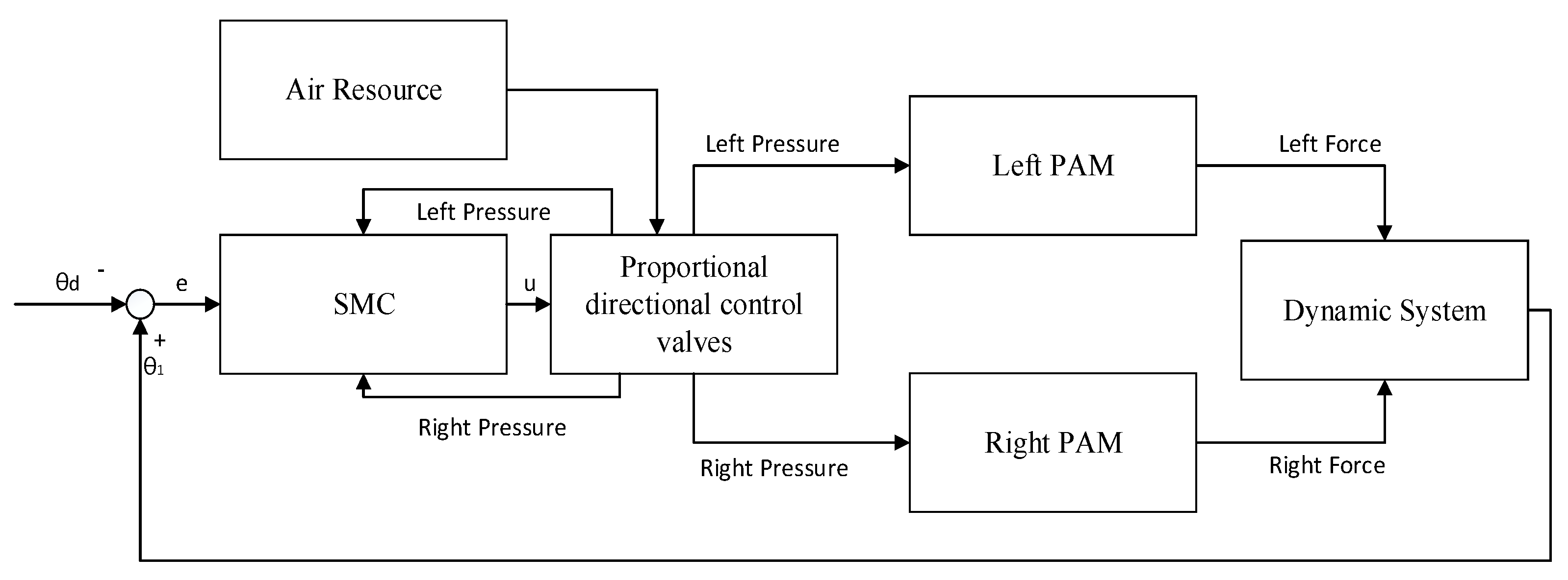
This section will introduce the controller and the parameter configurations of the controller used in this study. The fundamental concept of SMC is to force the system to enter a predesigned sliding plane. At the beginning, the system moves toward the plane, and then slides to the target point of control once entering the plane. As a result, for SMC a different sliding plane design will end in different effects on the system. The study designs a high-order SMC feedback controller [4]; the flow chart of the system control is shown in Figure 4.
The error of angle : is the trajectory of the tracking angle, and u is the control voltage command. The sliding plane for the high-order sliding-mode control (HOSMC) designed in this research is represented in Equation (21):
In SMC, the control command can be decomposed into the equivalent control law and the switching control law, which can be represented by Equation (22):
where represents the equivalent control law of HOSMC, and the switching control law. The equivalent control law defines the first derivative on a sliding plane to be 0, which is Equation (23):
Use Equations (21) to (23), and then combine with Equation (19), and the equivalent control law equation of HOSMC can be obtained, as in Equation (24):
where and : and are the simulated estimates from and . As for the part of the switching control law, the study uses the concept of a sliding layer proposed by Slotine (1983), so the switching control law equation is to be designed as Equation (25):
where is the width of the saturation region. From Equation (25), a sliding plane can be observed, which consists of two parts: the first one is the nonsaturation region , and the second one is the saturation region . The main purpose for designing the saturation region is to avoid vibration occurrence. When the system is in the nonsaturation region, the control law is selected as and as on the contrary. This method is able to effectively shrink the switching intensity within the saturation region, in which the width configuration of the saturation region can be satisfying if only a high-frequency vibration does not occur in the system.
Referring to the literature [5], the dynamic model of this system is represented as Equation (16); however, since the parameters of a robot arm cannot be accurately measured, it is modified to Equation (26):
where and represent the uncertainties of the dynamic system, and d is the external disturbance.
The influence brought by the uncertainties and external disturbance can be written as Equation (27):
Use Equation (27) into Equation (26); then the estimated dynamic model can be modified as Equation (28):
Use Equation (22) into Equation (26); then we can obtain Equation (29):
Eventually, we use Equation (29) into the sliding plane for the first derivative, and then we can acquire Equation (30):
To prove whether the high-order sliding-model designed in this study can stabilize the system controlled, as well as maintain the error of control on of the sliding plane, a Lyapunov function is selected as Equation (31):
Differentiate in regard to time, and we can obtain Equation (32).
Use Equation (30) into Equation (32), and then we can obtain Equation (33).
From the preceding descriptions, it is shown that when a system is under conditions with max uncertainties and external disturbance, and the value of exceeds the uncertainties and external disturbance of the system, a Lyapunov function is capable of guaranteeing that the trajectory tracking to the SMC system will be restrained on the sliding plane.
After building the dynamic model of the robot arm, the parameter identification of the controller is discussed next. In order to prevent the parameter adjustment in the experiment from diverging the system, as well as reduce the adjustment time, this study utilizes a real-number genetic algorithm to search the parameters of each controller (for introduction on genetic algorithm, please see Section 2.3.2) to define the criteria of reference for the experimental adjustment. To find out the parameters of each controller, this study adopts the closed-loop method by inputting the default values of the system model of the robot arm and the commands of trajectory tracking to calculate the optimal solution for the control command.
Because the robot arm is activated to act by the pulling of the two PAM cylinders with each other, where the inner force shrinks the MAX swing amplitude designed by the original mechanism (the swing amplitude originally designed is ±15°), a ±0.22 rad (=12.605°) sine trajectory is used as our target trajectory to simulate the possible trajectories carried out in the future. Therefore, the main purpose of this study for using the controller is to control the angle and to ensure the controllability of the robot arm under the two extreme statuses (min and MAX status on the R axis). Hence, the fitness function used to pursue the optimal solution is defined as the sums of the RMSE of the angles under the two aforementioned extreme statuses. The control variables of HOSMC are shown in Equations (24) and (25), which include λ, G, and . If the fitness function is defined through the RMSE of angle, the range of parameter identification and the outcomes can be acquired as shown in Table 5. The configuration of a genetic algorithm includes sampling number at 500, algebra at 1000, mutation rate at 0.4, and mating rate at 0.6.
Use the optimal solutions into the simulation, and the outcomes can be obtained as the error of angle of the first axis (), and the RMSE is 0.0207° when the centers of mass of the second axis and the third axis of the robot arm are at the closest distance ( = 0). Besides, the RMSE of the error of angle of the first axis () is 0.1318° when the centers of mass of the second axis and the third axis of the robot arm are at the farthest distance ( = 180).
3. Results and Discussion
3.1. Experiment and Discussion on the Fixed Moment of Inertia of a Robot Arm
To investigate the two extreme statuses of a robot arm, experiment and discussion are needed. According to the information regarding the hardware specs, it is shown that the quickest response time of this controller is 8 ms. As a result, we will discuss the configuration of sampling time and the fixed moment of inertia of the theta control of a robot arm in this section.
3.1.1. Configuration of Sampling Time
This section utilizes HOSMC to investigate the influence on precision of trajectory tracking by sampling time. The trajectory in the experiment is a ±10° sine, where the controller is traditionally designed by adopting the switching control law. Hence, the width of the saturation region is 0, and the parameters of the controller are λ = 12.5 and G = 150 to be used for the comparison of influence when the sampling times are 20 ms and 10 ms, respectively. The summaries thereof are shown in Table 6. We can see that the lower the sampling time, the better the tracking. In conclusion, we decided to adopt 10 ms as our sampling time for the subsequent experiments.
3.1.2. Investigation on the Fixed Moment of Inertia of a Robot Arm Controller
This study investigates the fixed moment of inertia of a robot arm controller. The experimental conditions are established to control the theta axis of the system via HOSMC and PID controller. The preceding section discussed the tracking precision under two extreme statuses. However, regarding the real control of the robot arm, we cannot completely simulate the actual situations of a robot arm, such as friction of the robot arm, friction of the PAM cylinder fabrics, and inertia of the robot arm when oscillating. As a result, we will use the optimal solutions of HOSMC parameters as what we have obtained in Section 2.3.2 as the criteria for the adjustment on actually controlling the robot arm. The PID parameters were tuned by the Ziegler–Nichols rule. The tracking trajectory is a ±10° sine, where the moments of inertia under the two extreme statuses should be adjusted to = 36,000 and = 276,077, and the parameter configurations of each controller are shown in Table 7.
Through the aforementioned configurations, the experiment is performed under the conditions of the fixed moment of inertia of a robot arm, whose outcomes are shown in Table 8. The error of the HOSMC controller is smaller than that of the PID controller, in which the former also has a better performance on both a shorter axis and a longer axis, and the difference on a longer axis is even more significant.
3.2. Circular Trajectory Tracking Based on Robot Arm Control
This section enables a robot arm to perform circular trajectory tracking with dual axes simultaneously. The radius of the circle is configured at 100 mm, and the principle of judgment is on the contour error [15] of the circle. According to the equation of motion proposed in the preceding paragraphs, we can accord with inverse kinematics to acquire the trajectories for reference at and of the robot arm.
3.2.1. Outcomes at Zero Load
This experiment compares the performances at zero load of robot arm controllers; the axis represents the PID controller, where the parameter configurations are proportional is 3, integral is 0.12, and derivative is 0.04. The control parameter configurations of the axis are in Table 9. The results are shown in Table 10:
The results demonstrate that on the tracking circular trajectory, the performance is better on the controlling theta axis and circular trajectory if the PID controller is applied on the second axis () and collocates the HOSMC controller on the first axis (), compared with the PID controller.
3.2.2. Outcomes at a Lower Load
This experiment compares the performances of the circular trajectory tracking of each robot arm controller at a lower load, where the main purpose is to investigate the robustness of each controller through the disturbance incurred by the load when the robot arm is in motion. The parameter configurations of each controller are the same as the ones set in the preceding experiment at zero load, and an object is hung, whose weight is 0.91 kg; the results of control are shown in Table 11.
From the table above, it can be observed that every controller has a certain degree of robustness when tracking the circular trajectory under the condition of a lower load of a robot arm, and the HOSMC controller has a better performance. The experimental results are shown in Figure 5 and Figure 6.
From the discussion above, we are able to see that each controller has a certain level of robustness. To find the controller with better robustness, we additionally perform a rotation experiment on under the condition of and the longest radius of the robot arm and compare the HOSMC controller with the PID controller. The results demonstrate that the HOSMC controller has a better performance. It can be recognized from Table 12 that the robustness of the HOSMC controller is better than that of the PID controller when the robot arm is at a lower load. Hence, better tracking results can be obtained by applying the HOSMC controller in the robot arm.
4. Conclusions
The robot arm and the dynamic model of the PAM cylinder can be applied to the hardware structure of the combination of the PAM cylinder, robot arm, and proportional flow control servo valve, as well as to the circular trajectory tracking, the undefined parameters in the dynamic model acquired by a genetic algorithm, and the parameter identification of a high-order sliding-mode feedback controller. This essay compares a PID controller and an HOSMC controller in using the precision of circular trajectory tracking. The experimental outcomes show that the maximum error between the objective locus and the following locus is 11.3035 mm (5.65%) (HOSMC controller), which not only solves the uncertainty problem when building the model more effectively, but also enables the robotic arm to have superior performance when tracking.
Author Contributions
Conceptualization, C.-J.L. and C.-H.D.; methodology, C.-J.L.; software, T.-Y.S.; validation, H.-T.Y., W.-L.C. and T.-Y.S.; formal analysis, C.-H.D.; investigation, W.-L.C.; resources, C.-J.L.; data curation, H.-T.Y.; writing—original draft preparation, W.-L.C.; writing—review and editing, C.-J.L.; visualization, C.-J.L.; supervision, C.-J.L.; project administration, C.-J.L.; funding acquisition, C.-J.L. All authors have read and agreed to the published version of the manuscript.
Funding
This research was funded by Ministry of Science and Technology of the Republic of China, Taiwan for financially/partially supporting, grant number MOST 108-2221-E-027-112-MY3 and The APC was funded by MOST 108-2221-E-027-112-MY3.
Institutional Review Board Statement
Not applicable.
Informed Consent Statement
Informed consent was obtained from all subjects involved in the study.
Data Availability Statement
Not applicable.
Conflicts of Interest
The authors declare no conflict of interest.
References
- Brahmi, B.; Saad, M.; Rahman, M.H.; Ochoa-Luna, C. Cartesian trajectory tracking of a 7-DOF exoskeleton robot based on human inverse kinematics. IEEE Trans. Syst. Man Cybern. Syst. 2019, 49, 600–611. [Google Scholar] [CrossRef]
- Kubota, S.; Abe, T.; Kadone, H.; Fujii, K.; Shimizu, Y.; Marushima, A.; Ueno, T.; Kawamoto, H.; Hada, Y.; Matsumura, A.; et al. Walking ability following hybrid assistive limb treatment for a patient with chronic myelopathy after surgery for cervical ossification of the posterior longitudinal ligament. J. Spinal Cord Med. 2019, 42, 128–136. [Google Scholar] [CrossRef] [PubMed]
- Kwakkel, G.; Kollen, B.J.; Krebs, H.I. Effects of robot-assisted therapy on upper limb recovery after stroke: A systematic review. Neurorehabil. Neural Repair 2008, 22, 111–121. [Google Scholar] [CrossRef]
- Riener, R.; Nef, T.; Colombo, G. Robot-aided neurorehabilitation of the upper extremities. Med. Biol. Eng. Comput. 2005, 43, 2–10. [Google Scholar] [CrossRef] [PubMed] [Green Version]
- Veerbeek, J.M.; van Wegen, E.; van Peppen, R.; van der Wees, P.J.; Hendriks, E.; Rietberg, M.; Kwakkel, G. What is the evidence for physical therapy poststroke? A systematic review and meta-analysis. PLoS ONE 2014, 9, e87987. [Google Scholar] [CrossRef] [PubMed] [Green Version]
- Pollock, A.; Farmer, S.E.; Brady, M.C.; Langhorne, P.; Mead, G.E.; Mehrholz, J.; van Wijck, F. Interventions for improving upper limb function after stroke. Cochrane Database Syst. Rev. 2014, CD010820. [Google Scholar] [CrossRef] [PubMed]
- Daerden, F.; Lefeber, D.; Verrelst, B.; Van Ham, R. Pleated pneumatic artificial muscles: Actuators for automation and robotics. In Proceedings of the 2001 IEEE/ASME International Conference on Advanced Intelligent Mechatronics, Como, Italy, 8–12 July 2001; pp. 738–743. [Google Scholar]
- Chou, C.P.; Hannaford, B. Measurement and modeling of McKibben pneumatic artificial muscles. IEEE Trans. Robot. Autom. 1996, 12, 90–102. [Google Scholar] [CrossRef] [Green Version]
- Huang, J.; Cao, Y.; Xiong, C.H.; Zhang, H.T. An echo state gaussian process-based nonlinear model predictive control for pneumatic muscle actuators. IEEE Trans. Autom. Sci. Eng. 2019, 16, 1071–1084. [Google Scholar] [CrossRef]
- Xie, S.-L.; Liu, H.-T.; Mei, J.-P.; Gu, G.-Y. Modeling and compensation of asymmetric hysteresis for pneumatic artificial muscles with a modified generalized Prandtl–Ishlinskii model. Mechatronics 2018, 52, 49–57. [Google Scholar] [CrossRef]
- Yang, H.; Chen, Y.; Sun, Y.; Hao, L. A novel Kriging-median inverse compensator for modeling and compensating asymmetric hysteresis of pneumatic artificial muscle. Smart Mater. Struct. 2018, 27, 115019. [Google Scholar] [CrossRef]
- Cveticanin, L.; Zukovic, M.; Biro, I.; Sarosi, J. Mathematical investigation of the stability condition and steady state position of a pneumatic artificial muscle-Mass system. Mech. Mach. Theory 2018, 125, 196–206. [Google Scholar] [CrossRef]
- Kalita, B.; Dwivedy, S.K. Nonlinear dynamics of a parametrically excited pneumatic artificial muscle (PAM) actuator with simultaneous resonance condition. Mech. Mach. Theory 2019, 135, 281–297. [Google Scholar] [CrossRef]
- Chen, Y.L.; Zhang, J.H.; Gong, Y.J. Novel design and modeling of a soft pneumatic actuator based on antagonism mechanism. Actuators 2020, 9, 107. [Google Scholar] [CrossRef]
- Martens, M.; Boblan, I. Modeling the static force of a festo pneumatic muscle actuator: A new approach and a comparison to existing models. Actuators 2017, 6, 33. [Google Scholar] [CrossRef] [Green Version]
- Anh, H.P.H.; Son, N.N.; Kien, C.V. Adaptive neural compliant force-position control of serial PAM robot. J. Intell. Robot. Syst. 2018, 89, 351–369. [Google Scholar] [CrossRef]
- Anh, H.P.H.; Kien, C.V.; Son, N.N.; Nam, N.T. New approach of sliding mode control for nonlinear uncertain pneumatic artificial muscle manipulator enhanced with adaptive fuzzy estimator. Int. J. Adv. Robot. Syst. 2018, 15, 1729881418773204. [Google Scholar] [CrossRef]
- Nguyen, H.T.; Trinh, V.C.; Le, T.D. An adaptive fast terminal sliding mode controller of exercise-assisted robotic arm for elbow joint rehabilitation featuring pneumatic artificial muscle actuator. Actuators 2020, 9, 118. [Google Scholar] [CrossRef]
- Minh, T.V.; Tjahjowidodo, T.; Ramon, H.; Van Brussel, H. Cascade position control of a single pneumatic artificial muscle-mass system with hysteresis compensation. Mechatronics 2010, 20, 402–414. [Google Scholar] [CrossRef]
- Luk’yanov, A.; Dodds, S.; Vittek, J. Observer-based attitude control in the sliding mode. Trans. Built Environ. 1970, 22. [Google Scholar] [CrossRef]
- Sárosi, J.; Gyeviki, J.; Véha, A.; Toman, P. Accurate position control of PAM actuator in Lab VIEW environment. In Proceedings of the 2009 7th International Symposium on Intelligent Systems and Informatics, Subotica, Serbia, 25–26 September 2009; pp. 301–305. [Google Scholar]
- Shen, X.R. Nonlinear model-based control of pneumatic artificial muscle servo systems. Control Eng. Pract. 2010, 18, 311–317. [Google Scholar] [CrossRef]
- Furat, M.; Eker, I. Second-order integral sliding-mode control with experimental application. ISA Trans. 2014, 53, 1661–1669. [Google Scholar] [CrossRef] [PubMed]
Figure 1.
Structure of the electromechanical system of a robot arm.

Figure 2.
Transmission sketch of a robot arm.

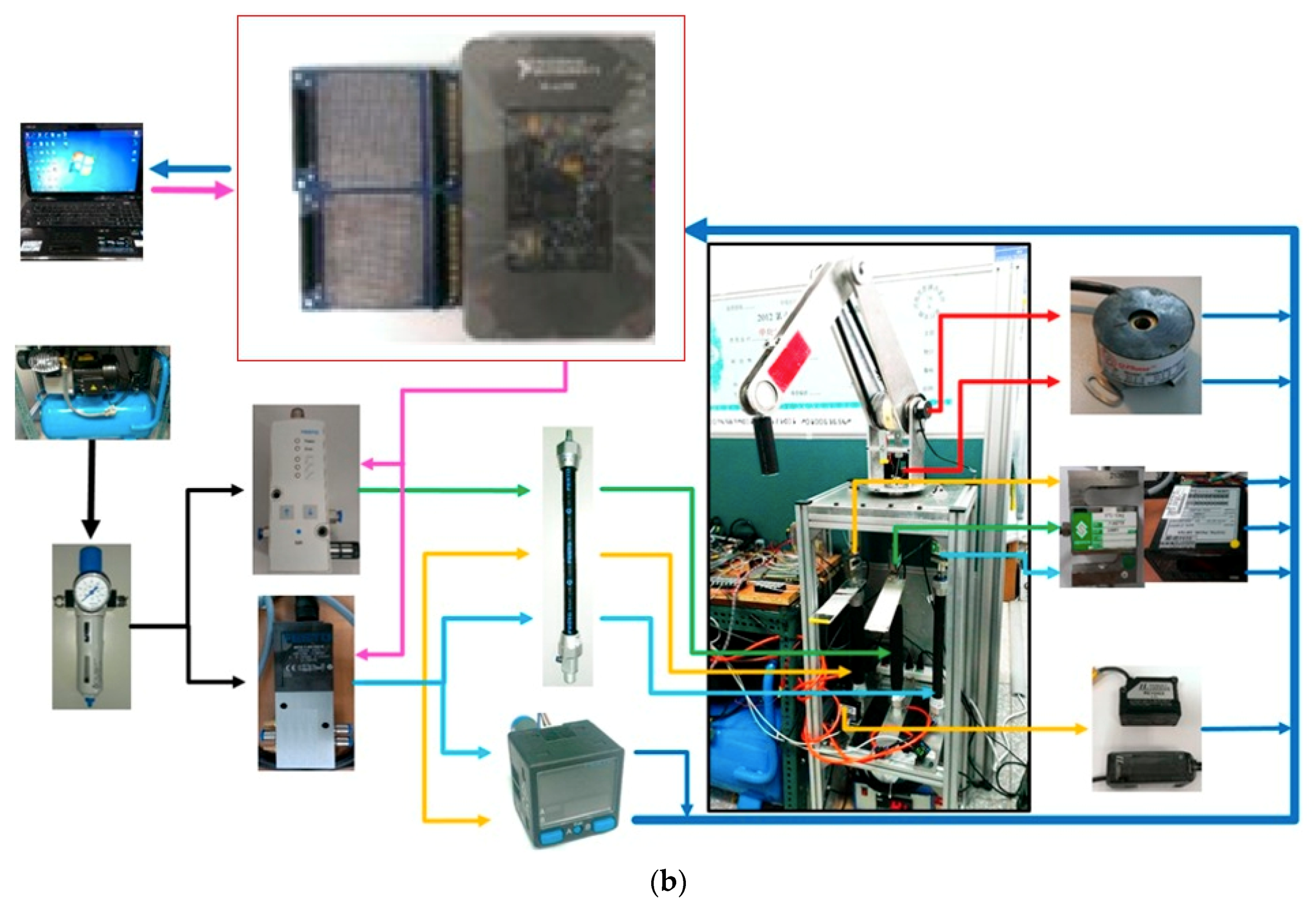
Figure 3.
(a) Transmission sketch of a robot arm, (b) experimental setup.


Figure 4.
Overall view of system and SMC feedback controller system graph.

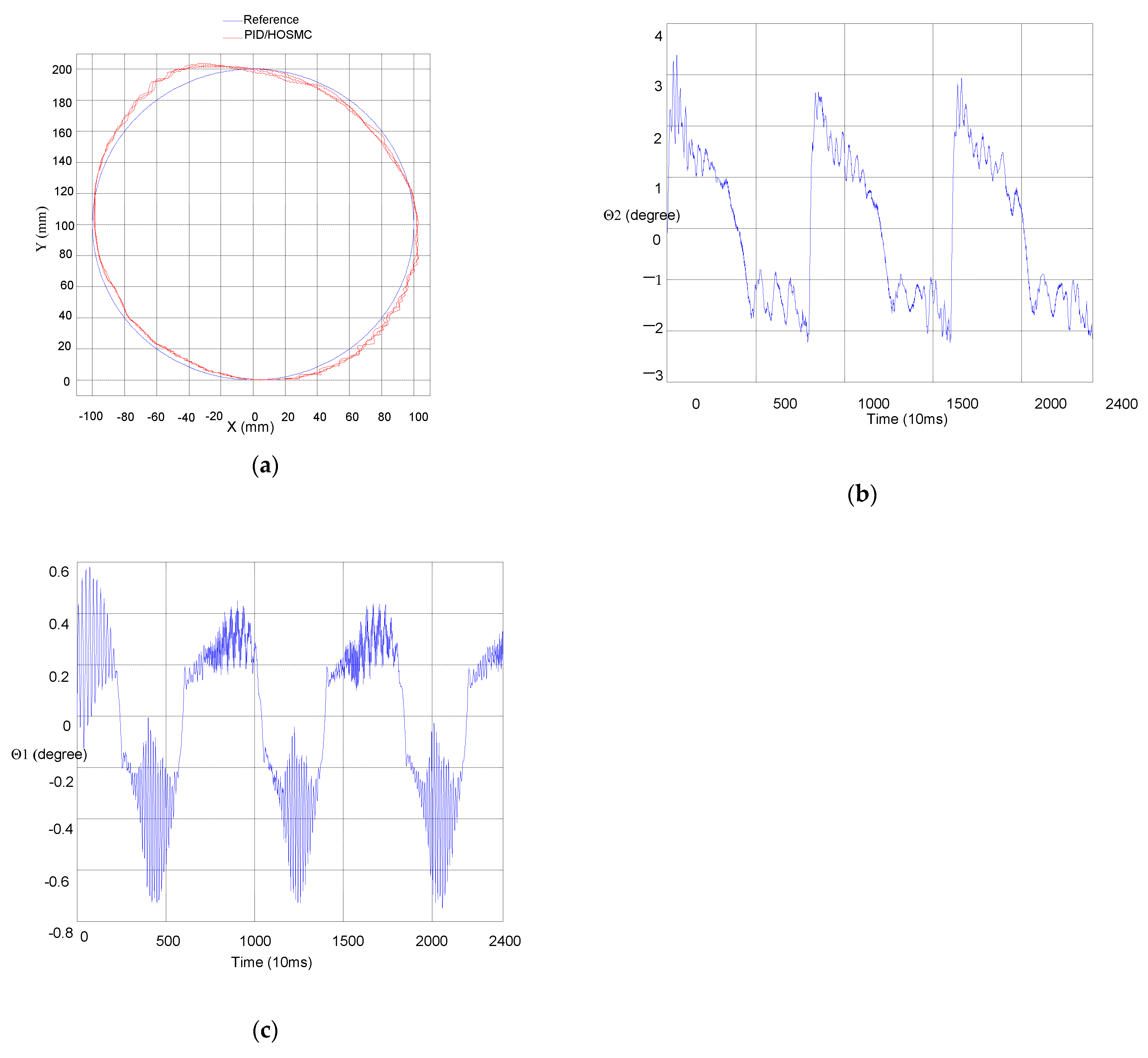
Figure 5.
Results of the tracking circular trajectory of a robot arm (the axis uses PID, and the axis uses HOSMC controllers): (a) results of the tracking circular trajectory of a robot arm (the axis uses PID, and the axis uses HOSMC controllers); (b) tracking error of the axis at a lower load; (c) tracking error of the axis at a lower load.

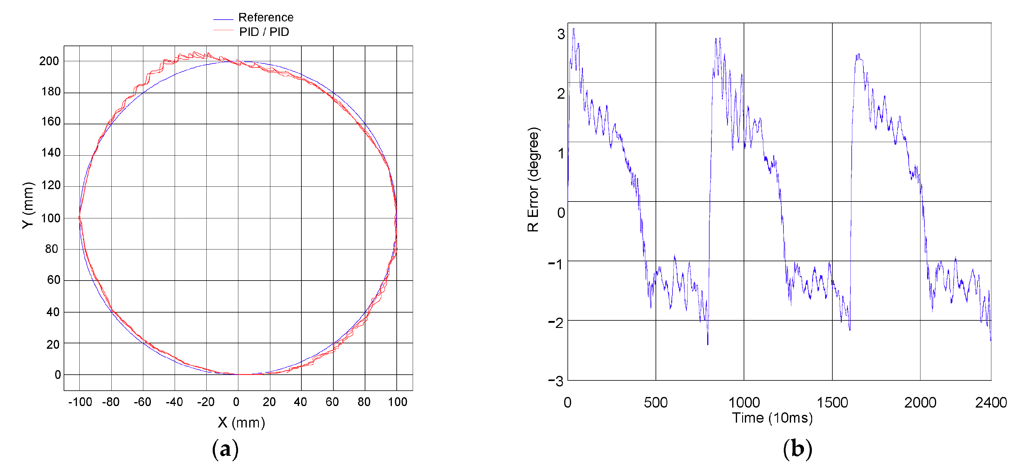
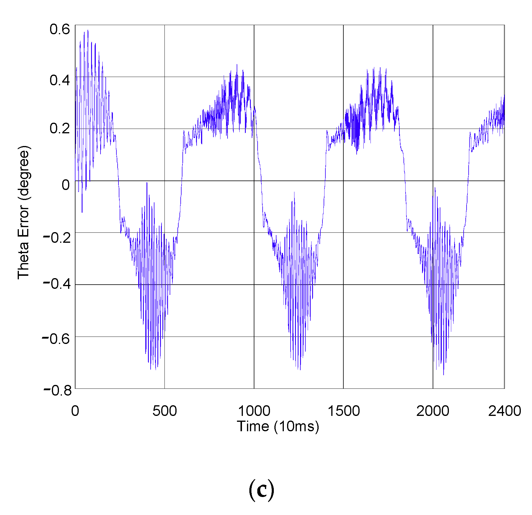
Figure 6.
Results of the tracking circular trajectory of a robot arm (the axis uses PID, and the axis uses axis uses PID): (a) results of the tracking circular trajectory of a robot arm (the axis uses PID, and the axis uses PID); (b) tracking error of the axis at a lower load; (c) tracking error of the axis at a lower load.


Table 1.
Spec list of hardware and equipment used in this study.
| Item | Type | Specifications |
|---|---|---|
| Proportional flow control servo valve | Developed by Festo (MPYE-5-M5-010-B) | Standard nominal flow rate (L/min): 100 Product weight (g): 290 (not containing connectors) |
| PRV | Developed by Festo (VPPM-6L-L-1-G18-0L10H-V1N) | Pressure range: 0 to 10 bar Input voltage range: 0 to 10 V Feedback voltage by pressure range: 0 to 10 V |
| PAM cylinder | Developed by Festo (MAS-20-300N-AA-MC-O-ER-BG) | The structure includes a contractile system and a connector of two ends, where the inside of the contractile system is a hose, and the outside is covered by a fabric mesh with high intensity. |
| Power sensor | Developed by VPG load cell | A correspondent voltage generated by deformation due to the extension of the load cell can be obtained, where the force measure range is from 0 to 100 kg, and the feedback voltage signal is from 0 to 10 V. |
| Pressure sensor | Developed by Festo (SPAB-P10R-G18-NB-K1) | Pressure measure range: 0 to 10 bar Feedback voltage signal: 1 to 5 V |
| Optical encoder | Developed by QPhase (TSD-HB-8-1000A-H) | Can be utilized for the analysis of frequency quadruple, where the resolution of one cycle is 8000 Hz. |
| Laser rangefinder | Developed by Keyence Type of IL-300 | Measure distance: 300 mm Measure range: 160 to 450 mm Precision of measure repeatability: 30 µm Output voltage range: 0 to 5 V |
Table 2.
D–H parameters of a robot arm.
| θ | d | a | α |
|---|---|---|---|
| 0 | 0 | 90° | |
| 0 | 0° | ||
| 0 | 0° |
Table 3.
Parameter table of the model of the proportional flow control servo valve.
| Parameter | Units | Value | Range |
|---|---|---|---|
| 101.3 | – | ||
| 707 | – | ||
| γ | – | 1.4 | – |
| R | 0.287 | – | |
| T | 293 | – | |
| – | 0–30,000 | ||
| – | 200,000–400,000 | ||
| B | – | 0–10,000 | |
| Gain | – | – | 0.8–1.2 |
| – | 250–255 | ||
| D | – | 20–40 | |
| b | – | 250–441.673 | |
| – | – | 0–1 | |
| – | – | 0.143–1 |
Table 4.
Range of parameter configuration of a dynamic model of a robot arm and optimal parameter.
| Gene | Range | Optimum Parameter |
|---|---|---|
| 0 to 30,000 | 15,960.7 | |
| 200,000 to 400,000 | 267,077 | |
| B | 0 to 10,000 | 7042.55 |
| 250 to 255 | 252.446 | |
| D | 20 to 40 | 35.406 |
| b | 250 to 441.673 | 385.02 |
| 0 to 1 | 0.0889213 | |
| 0.14268 to 1 | 0.538054 | |
| 0.8 to 1.2 | 0.988137 |
Table 5.
Range of optimal controller parameters and outcomes.
| Parameter | Range | Optimum Parameter |
|---|---|---|
| Λ | 0 to 100 | 17.6953 |
| G | 0 to 10,000 | 384.302 |
| 0 to 10,000 | 776.93 |
Table 6.
Comparison table of tracking outcomes at different sampling times.
| Sampling Time | Max Error (Degree) | RMSE (Degree) |
|---|---|---|
| 20 ms | 2.089 | 0.51468 |
| 10 ms | 0.402 | 0.12895 |
Table 7.
Parameter configurations of the controller of the fixed moment of inertia.
| Controller | Controller Parameters |
|---|---|
| HOSMC | , , |
| PID | , , |
Table 8.
Comparison table of controlling fixed moment of inertia of a robot arm.
| Controller | State | Max Error (Degree) | RMSE (Degree) |
|---|---|---|---|
| HOSMC | Short | 0.448 | 0.11126 |
| Long | 0.381 | 0.090299 | |
| PID | Short | 0.523 | 0.25232 |
| Long | 0.706 | 0.289 |
Table 9.
Parameter table of the theta axis controller of a manipulator with fixed rotation inertia control.
Table 9.
Parameter table of the theta axis controller of a manipulator with fixed rotation inertia control.
| Controller | Controller Parameters |
|---|---|
| HOSMC | , , |
| 2-SMC | , , , |
| TSMC | , , , , , |
| PID | , , |
Table 10.
Comparison table of the tracking results on the circular trajectory at zero load based on theta axis control.
Table 10.
Comparison table of the tracking results on the circular trajectory at zero load based on theta axis control.
| Controller | Part | Max Error | RMSE |
|---|---|---|---|
| PID/HOSMC | (degree) | 0.524 | 0.14781 |
| Contour (mm) | 10.2528 | 3.6808 | |
| PID/PID | (degree) | 0.768 | 0.30876 |
| Contour (mm) | 10.0909 | 2.9096 |
Table 11.
Comparison table of the tracking results on the circular trajectory at a lower load of an robot arm.
Table 11.
Comparison table of the tracking results on the circular trajectory at a lower load of an robot arm.
| Controller | Part | Max Error | RMSE |
|---|---|---|---|
| PID/HOSMC | (degree) | 0.524 | 0.14781 |
| Contour (mm) | 10.2528 | 3.6808 | |
| PID/PID | (degree) | 0.768 | 0.30876 |
| Contour (mm) | 10.0909 | 2.9096 |
Table 12.
Comparison table of robustness investigation between different robot arm controllers at a lower load.
Table 12.
Comparison table of robustness investigation between different robot arm controllers at a lower load.
| Controller | Max Error (Degree) | RMSE (Degree) |
|---|---|---|
| HOSMC | 0.399 | 0.10167 |
| PID | 4.086 | 1.6673 |
Publisher’s Note: MDPI stays neutral with regard to jurisdictional claims in published maps and institutional affiliations. |
© 2021 by the authors. Licensee MDPI, Basel, Switzerland. This article is an open access article distributed under the terms and conditions of the Creative Commons Attribution (CC BY) license (http://creativecommons.org/licenses/by/4.0/).
Share and Cite
MDPI and ACS Style
Lin, C.-J.; Sie, T.-Y.; Chu, W.-L.; Yau, H.-T.; Ding, C.-H. Tracking Control of Pneumatic Artificial Muscle-Activated Robot Arm Based on Sliding-Mode Control. Actuators 2021, 10, 66. https://0-doi-org.brum.beds.ac.uk/10.3390/act10030066
AMA Style
Lin C-J, Sie T-Y, Chu W-L, Yau H-T, Ding C-H. Tracking Control of Pneumatic Artificial Muscle-Activated Robot Arm Based on Sliding-Mode Control. Actuators. 2021; 10(3):66. https://0-doi-org.brum.beds.ac.uk/10.3390/act10030066
Chicago/Turabian StyleLin, Chih-Jer, Ting-Yi Sie, Wen-Lin Chu, Her-Terng Yau, and Chih-Hao Ding. 2021. "Tracking Control of Pneumatic Artificial Muscle-Activated Robot Arm Based on Sliding-Mode Control" Actuators 10, no. 3: 66. https://0-doi-org.brum.beds.ac.uk/10.3390/act10030066
Note that from the first issue of 2016, this journal uses article numbers instead of page numbers. See further details here.