
A Global Optimization Method to Determine the Complex Material Constants of Piezoelectric Bars in the Length Thickness Extensional Mode


1
The Program in Applied and Computational Mathematics, Princeton University, Princeton, NJ 08544, USA
2
School of Power and Mechanical Engineering, Wuhan University, Wuhan 430072, China
*
Author to whom correspondence should be addressed.
Actuators 2021, 10(8), 169; https://0-doi-org.brum.beds.ac.uk/10.3390/act10080169
Submission received: 23 May 2021
/
Revised: 12 June 2021
/
Accepted: 13 June 2021
/
Published: 22 July 2021
(This article belongs to the Special Issue Advances in Piezoelectric Actuators 2022)
Abstract
:Optimization methods have been used to determine the elastic, piezoelectric, and dielectric constants of piezoelectric materials from admittance or impedance measurements. The optimal material constants minimize the difference between the modeled and measured admittance or impedance spectra. In this paper, a global optimization method is proposed to calculate the optimal material constants of piezoelectric bars in the length thickness extensional mode. The algorithm is applied to a soft PZT and a hard PZT and is shown to be robust.
1. Introduction
Piezoelectric constants and are indispensable parameters when we evaluate the performances of new piezoelectric materials. A common method to determine from capacitance and admittance measurements has been described in an IEEE standard [1]. First, the dielectric constant is calculated from the capacitance measured at 1 kHz. Second, the elastic compliance constant is calculated from the frequency of maximum conductance in the length thickness extensional mode. Third, the electromechanical coupling factor is calculated from and the frequency of maximum resistance . The piezoelectric constant is finally calculated from , , and [1].
To circumvent the need of the capacitance measurement, researchers have developed iterative and non-iterative methods to determine the material constants (, , and ) from only the admittance measurements in the length thickness extensional mode. Smits proposed an iterative method to calculate the complex material constants from the admittances at three frequencies [2]. According to the one-dimensional model in the IEEE standard [1], the three complex admittances suffice to determine the three complex material constants [3], whose imaginary parts represent the losses in the material [4]. Smits’s method involved the manual selection of three data points on an admittance curve, which was later automated by Alemany et al. [3]. Non-iterative methods have also been proposed to calculate the material constants from particular near-resonance frequencies and the corresponding admittances [5,6].
In contrast to the iterative and non-iterative methods that use a limited number of admittance data, fitting methods are based on the whole admittance spectra and are therefore robuster. In a fitting method, the material constants are determined by fitting the modeled admittance or impedance spectra to the measurements. The optimal material constants are those that minimize the difference between the modeled and measured admittance or impedance spectra.
When the modeled admittance or impedance spectra come from the one-dimensional model of the length thickness extensional mode, the optimal material constants can be calculated with local optimization algorithms, such as the simplex algorithm [7], the Levenberg–Marquardt algorithm [8], and the Nelder–Mead algorithm [9]. Unlike the global optimization algorithms that were recently proposed for the thickness extensional mode [10] and the radial mode [11], these local optimization algorithms may not converge to the globally optimal material constants, especially when the initial guess of the material constants is inaccurate. To propose a global optimization algorithm for the length thickness extensional mode is the first motivation of this paper.
The modeled admittance or impedance spectra in the fitting methods can also come from finite element simulations [12,13,14,15,16]. Finite element simulations are able to predict the admittance at any frequency, even when different vibration modes are coupled. On the contrary, each one-dimensional model only applies to a specific vibration mode. Furthermore, one-dimensional models are only valid for samples with particular shapes and dimensions. The constraint is unnecessary in the finite element simulations. The fitting methods based on finite element simulations, however, are too complicated to be used in everyday research for most researchers.
Although there are several fitting methods based on the one-dimensional model of the length thickness extensional mode [7,8,9], no open-source software is available. Consequently, researchers have to write their own code to realize the algorithms if they cannot afford a commercial software license [17]. The second motivation of this paper is to publish an open-source code to determine the material constants in the one-dimensional model of the length thickness extensional mode.
The global optimization method proposed in this paper has the following advantages over other methods. It does not need a capacitance measurement to determine the dielectric constant , in contrast to the common method in the IEEE standard [1]. Unlike the iterative and non-iterative methods [2,3,5,6], our method takes full advantage of the measured admittance spectra and is less prone to experimental errors. Compared with the local optimization methods [7,8,9], the present global optimization method is able to find the globally optimal material constants even when their initial guesses are chosen randomly. Based on the one-dimensional model, the present method is more efficient and convenient than the fitting methods based on finite element simulations [12,13,14,15,16].
This paper is arranged as follows. In Section 2, we introduce the global optimization method to fit the modeled admittance and impedance spectra to the measured ones. The algorithm is applied to calculate the optimal material constants of PZT materials and the results are presented in Section 3 and discussed in Section 4. Conclusions are given in Section 5.
2. Materials and Methods
In the one-dimensional model of the length thickness extensional mode, the electrical admittance of a rectangular bar is [1]:
where and f is the frequency of the driving voltage. The density (), length (l), width (w), and thickness (t) of the bar are experimentally measured. The one-dimensional model applies when and [1]. The admittance also depends on an elastic compliance constant (), a dielectric constant (), and a piezoelectric constant () of the material. The three material constants are assumed to be complex numbers. The imaginary parts of , , and are related to the elastic, dielectric, and piezoelectric losses, respectively [4]. The six-dimensional real vector is defined as:
where “” and “” represent the real and imaginary parts, respectively. The superscript “” represents the transpose of the vector.
The experimental admittances are denoted as , where () are N frequencies around the resonance frequency of the first length thickness extensional mode. We denote the average relative error of the admittance and impedance in the one-dimensional model as
where
Here, , , , , and are the conductance, susceptance, impedance, resistance, and reactance, respectively. The subscripts “” and “” represent the modeled and measured quantities, respectively. The optimal material constants correspond to the vector that minimizes the average relative error . The minimum average relative error is calculated with the Levenberg–Marquardt modification of Newton’s method as follows [18].
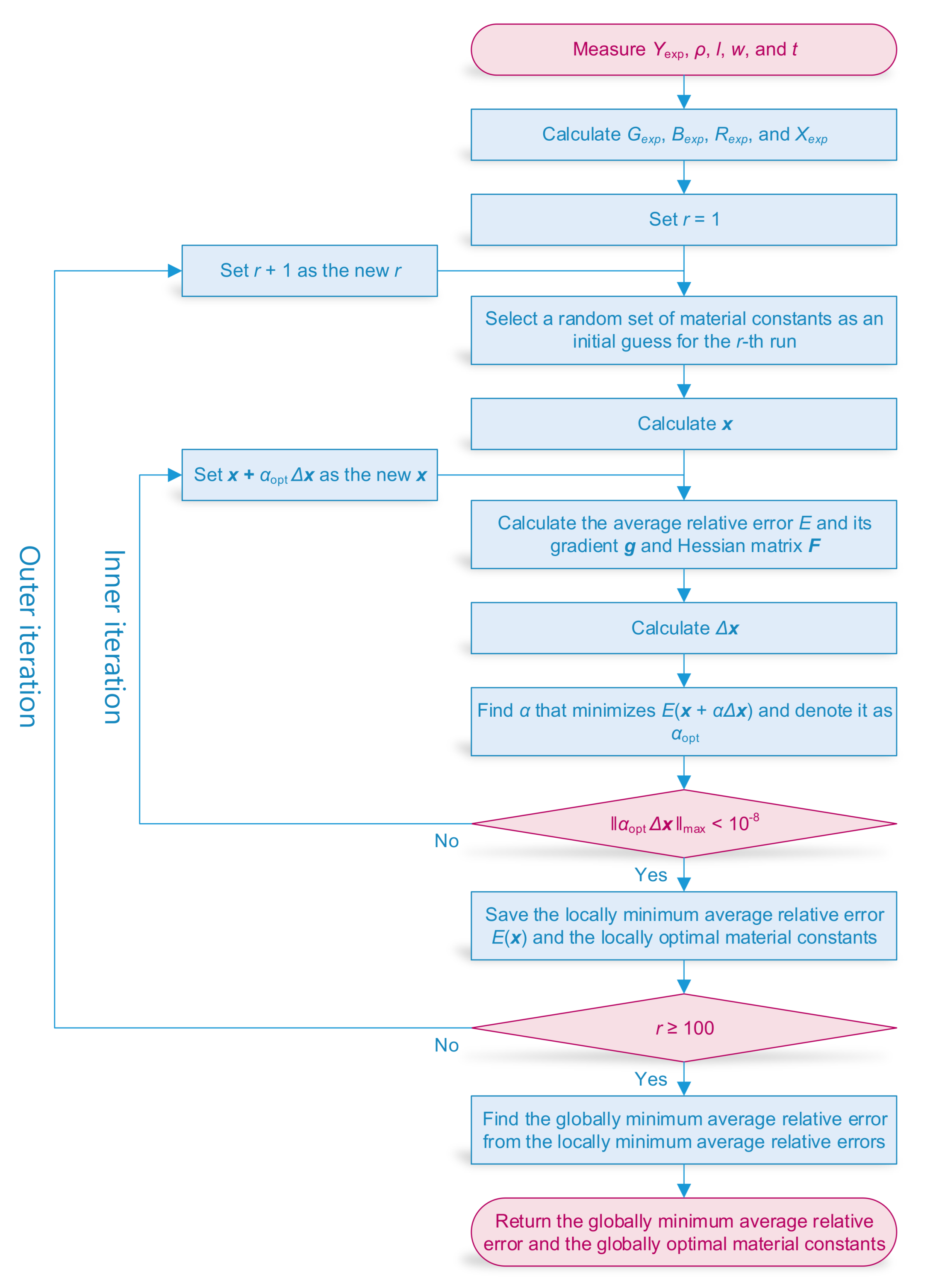
- (1)
- Measure the admittance, density, and dimensions of the sample. Calculate the experimental conductance, susceptance, resistance, and reactance from the measured admittance.
- (2)
- Randomly select a set of material constants as an initial guess, where:
- (3)
- Define:such that the absolute value of each component of is close to 1.
- (4)
- Calculate the average relative error E from Equations (3)–(7). Note that E is also a function of . Calculate the gradient and the Hessian matrix of E and denote them as and , whose expressions are derived in Appendix A.
- (5)
- Define , where and is the minimum eigenvalue of the Hessian matrix . is the identity matrix.
- (6)
- Calculate the average relative errors for step sizes , 1/5, 1, and 5. Find the minimum average relative error , where is the optimal step size. Take to be the new .
- (7)
- In the inner iteration, repeat steps 4–6 until the absolute values of all components of are less than . Then is the locally minimum average relative error. Calculate the locally optimal material constants from Equation (14).
- (8)
- In the outer iteration, repeat steps 2–7 for 100 times with different sets of initial material constants. The globally minimum average relative error is defined as the minimum among all locally minimum average relative errors. The corresponding material constants are the globally optimal material constants.
3. Results
The algorithm proposed in Section 2 is applied to a soft PZT and a hard PZT to calculate their optimal material constants in the length thickness extensional mode. The densities of the soft PZT and the hard PZT are kg/m3 and kg/m3, respectively [7]. Both samples have the same dimensions. The length, width, and thickness are 12 mm, 3 mm, and 1 mm, respectively [7].
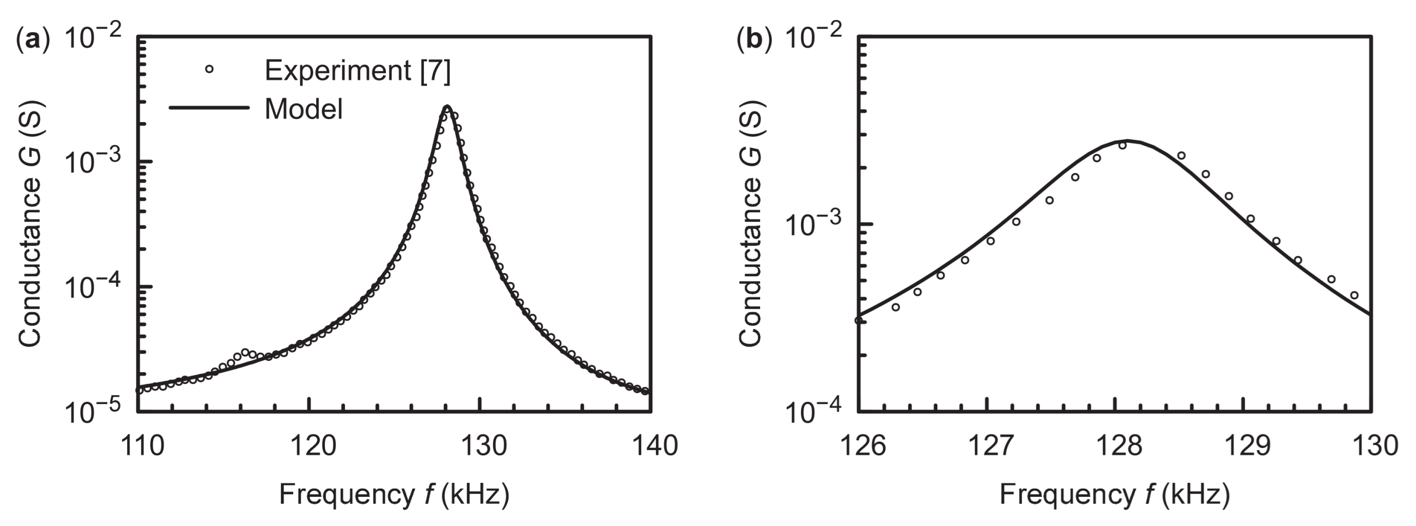
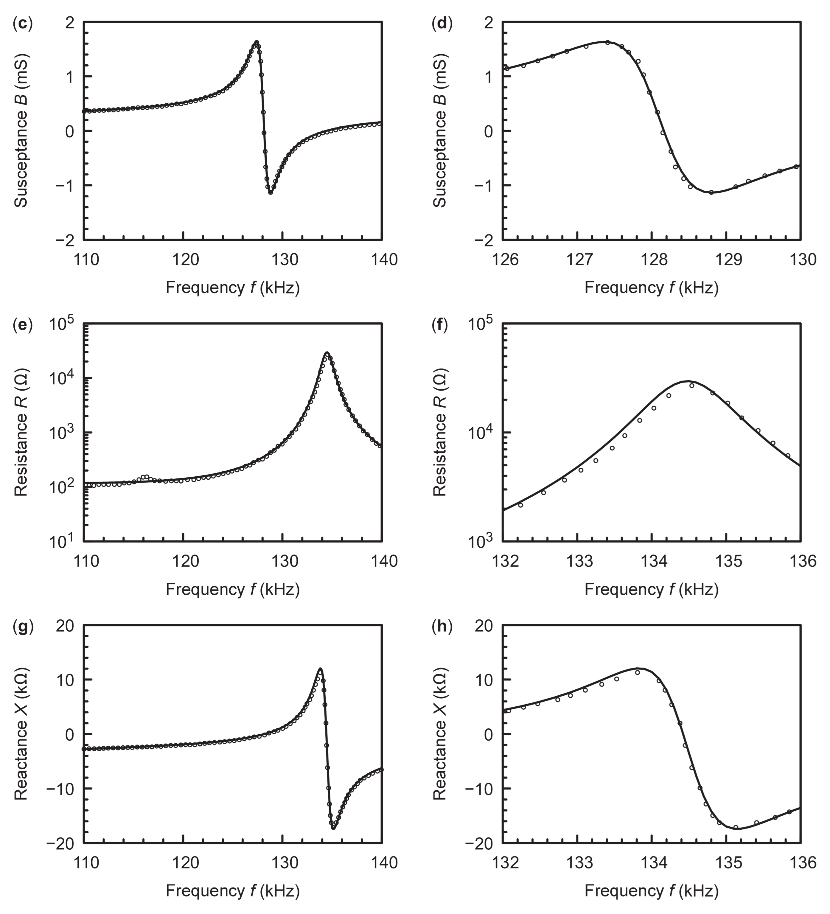
The experimental admittance and impedance of the soft PZT are obtained from Figure 1 in [7] and plotted with symbols in Figure 2. Note that the data are not evenly spaced in the frequency range between 110 kHz and 140 kHz, which corresponds to the first length thickness extensional mode. For example, the reactance data are denser when (Figure 2h). Consequently, we use the linearly interpolated admittance and impedance at 301 frequencies evenly spaced between 110 kHz and 140 kHz as the experimental data in our calculations. The modeled admittance and impedance that best fit the experimental data are then calculated with the present algorithm and plotted with lines in Figure 2. The globally minimum average relative error is 6.5% and is found in 40 runs among 100 runs with different initial material constants. The optimal material constants are listed in Table 1 and are confirmed to satisfy Equations (15)–(17). The relative differences between our results and the previous results [7] are less than 3% and 7% for the real and imaginary parts of the material constants, respectively.
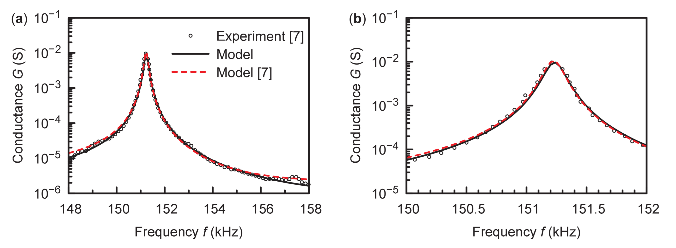
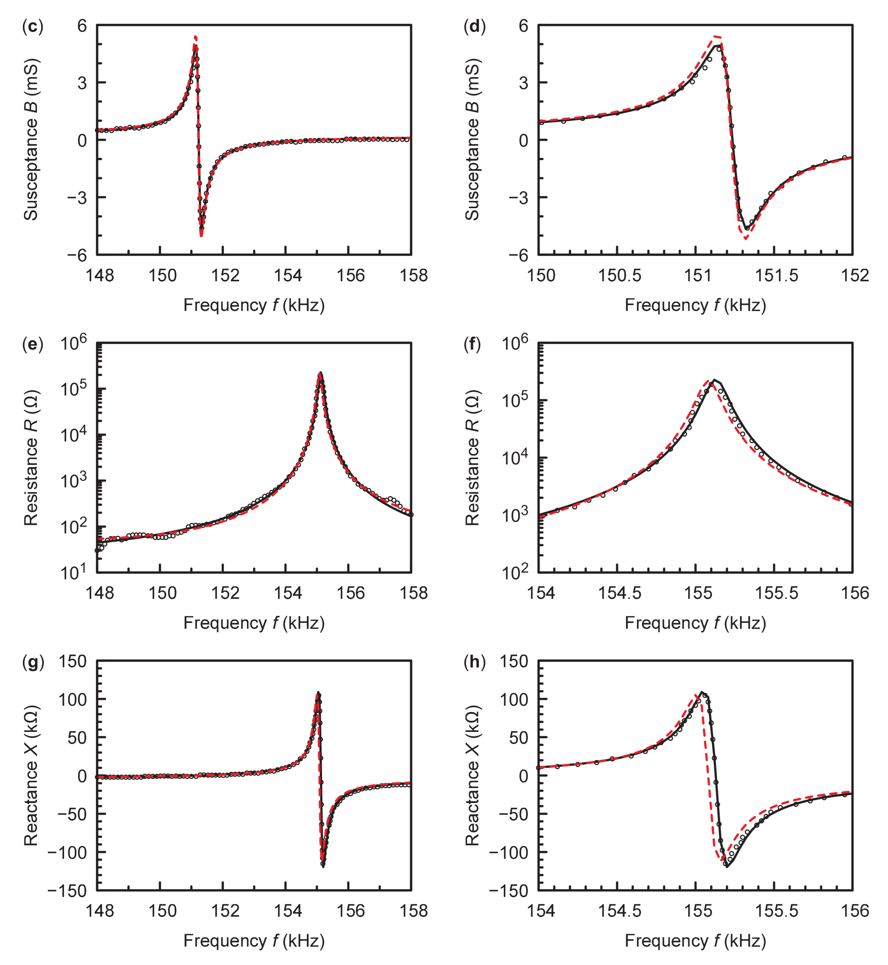
Similarly, the experimental admittance and impedance of the hard PZT in the first length thickness extensional mode at 251 frequencies evenly spaced between 148 kHz and 158 kHz are linearly interpolated from Figure 2 in [7]. The original experimental data and the best fitting curves are plotted in Figure 3 with symbols and lines, respectively. The globally minimum average relative error is 10.4% and is found in 48 runs among 100 runs. The optimal material constants are listed in Table 1 and are confirmed to satisfy Equations (15)–(17). The relative differences between our results and the previous results [7] are less than 7% for the real parts of the material constants. The imaginary parts of the present optimal and , however, do not agree with the previous results [7]. Compared with the previous best fitting results [7], which are plotted with red dashed lines in Figure 3, our best fitting admittance and impedance are closer to the experimental results.
4. Discussion
In Section 3, the minimum average relative errors are 6.5% and 10.4% for the soft PZT and the hard PZT, respectively. Note that these average relative errors represent the relative differences between the modeled admittance and impedance spectra and the measured ones. The errors of the optimal material constants are difficult to estimate but should be far less than 10%. Otherwise, the differences between the modeled and measured resonance frequencies would have been evident in Figure 2 and Figure 3.
The average relative error of the modeled admittance and impedance spectra cannot be reduced to zero due to the following two reasons. First, the measured admittance and impedance may not be accurate. They are sensitive to the holding position of the sample. Second, the one-dimensional model (Equation (1)) only applies when and [1]. When these conditions are not satisfied or when the sample is not a perfect rectangular bar, the one-dimensional model is only an approximation.
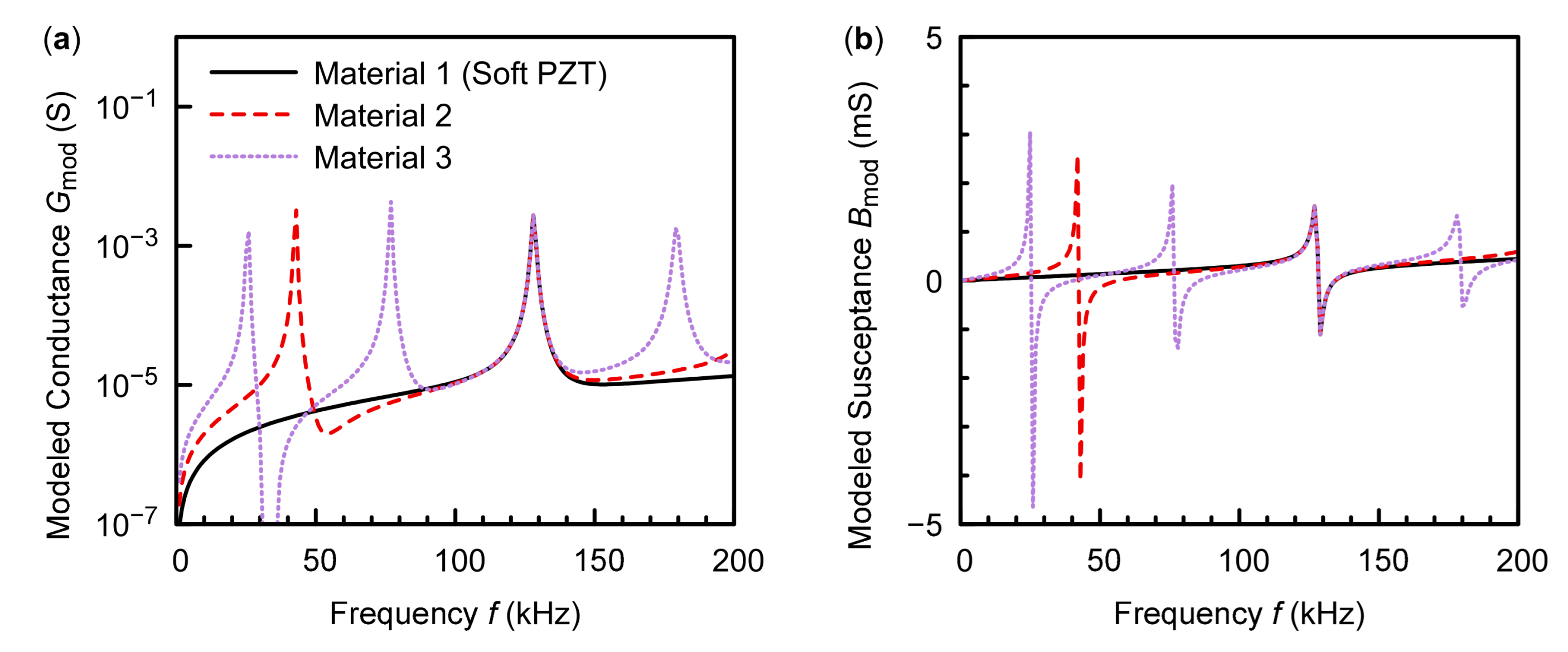
The present global optimization method depends on the range of the initial guess of material constants. If this range is larger than that in Equations (8)–(13), the algorithm may need more runs to find the globally optimal material constants. The algorithm may even find different locally optimal material constants that have almost the same average relative error. Actually, according to Theorem A1 in Appendix B, different materials may have similar admittances around the same resonance frequency. For example, if we have several materials and the material constants of the n-th material are , , and , where , then the n-th resonance frequency of the n-th material is close to the first resonance frequency of the first material. Furthermore, the admittance spectrum of the n-th material near its n-th resonance frequency is similar to that of the first material near the first resonance frequency. This phenomenon is illustrated in Figure 4, where the first material is chosen as the soft PZT.
Although the present algorithm may converge to different optimal material constants, we can easily check whether the vibration mode in the given frequency range is the first mode. According to Figure 4, those conductance spectra with local maxima at lower frequencies outside the given frequency range should be neglected. Only the optimal material constants that correspond to a modeled admittance spectrum with the first mode in the given frequency range are the ones we need.
5. Conclusions
In this paper, we proposed a global optimization method to determine the complex material constants of piezoelectric bars in the length thickness extensional mode. The calculated optimal material constants and the best fitting admittance and impedance are consistent with the previous results [7] for a soft PZT and a hard PZT. Unlike the previous algorithms [7,8,9], the present algorithm involved 100 runs from random initial material constants and was able to find the globally minimum average relative error of the modeled admittance and impedance. Even when the initial material constants were randomly chosen from a wide range, at least 40% of runs found the globally minimum average relative error, which shows the robustness of the current algorithm. On the contrary, the local optimization methods [7,8,9] depend on well-chosen initial material constants, otherwise they may find a local minimum instead of the global minimum of the average relative error.
The present algorithm can also be modified to determine the optimal material constants in other vibration modes with one-dimensional models.
Author Contributions
Conceptualization, X.X. and X.L.; methodology, X.X. and X.L.; software, X.X.; validation, X.X. and X.L.; formal analysis, X.X. and X.L.; investigation, X.X. and X.L.; resources, X.X. and X.L.; data curation, X.X. and X.L.; writing—original draft preparation, X.X.; writing—review and editing, X.X. and X.L.; visualization, X.X.; supervision, X.L.; project administration, X.L.; funding acquisition, X.L. All authors have read and agreed to the published version of the manuscript.
Funding
This research was funded by the National Natural Science Foundation of China grant number 51705373.
Data Availability Statement
The computer code developed in this study is written in MATLAB R2020a and is available at https://github.com/xiangmingxiong/length-thickness-extensional-vibration-analysis (accessed on 15 June 2021). The data presented in this study are openly available in Open Science Framework at doi:10.17605/OSF.IO/N8P7K.
Conflicts of Interest
The authors declare no conflict of interest. The funders had no role in the design of the study; in the collection, analyses, or interpretation of data; in the writing of the manuscript, or in the decision to publish the results.
Appendix A
Denoting the components of the gradient and the entries of the Hessian matrix as and (), we have:
according to Equations (2) and (14), where , , , , , and .
Noticing that is a holomorphic function of each complex material constant according to Equation (1), we have:
From , we have:
for and
for .
Appendix B
Theorem A1.
For any positive integer n,
when and , where:
References
- IEEE Standard on Piezoelectricit. ANSI/IEEE Std 176-1987, 1988. In Proceedings of the IEEE Computer Society Office Automation Symposium, National Bureau of Standards, Gaithersburg, MD, USA, 27–29 April 1987. [Google Scholar] [CrossRef]
- Smits, J.G. Iterative method for accurate determination of the real and imaginary parts of the materials coefficients of piezoelectric ceramics. IEEE Trans. Son. Ultrason. 1976, SU-23, 393–401. [Google Scholar] [CrossRef]
- Alemany, C.; Pardo, L.; Jiménez, B.; Carmona, F.; Mendiola, J.; González, A.M. Automatic iterative evaluation of complex material constants in piezoelectric ceramics. J. Phys. D Appl. Phys. 1994, 27, 148–155. [Google Scholar] [CrossRef]
- Holland, R. Representation of dielectric, elastic, and piezoelectric losses by complex coefficients. IEEE Trans. Son. Ultrason. 1967, SU-14, 18–20. [Google Scholar] [CrossRef]
- Sherrit, S.; Wiederick, H.D.; Mukherjee, B.K. Non-iterative evaluation of the real and imaginary material constants of piezoelectric resonators. Ferroelectrics 1992, 134, 111–119. [Google Scholar] [CrossRef]
- Du, X.H.; Wang, Q.M.; Uchino, K. Accurate determination of complex materials coefficients of piezoelectric resonators. IEEE Trans. Ultrason. Ferroelect. Freq. Contr. 2003, 50, 312–320. [Google Scholar] [CrossRef]
- Tsurumi, T.; Kil, Y.B.; Nagatoh, K.; Kakemoto, H.; Wada, S.; Takahashi, S. Intrinsic elastic, dielectric, and piezoelectric losses in lead zirconate titanate ceramics determined by an immittance-fitting method. J. Am. Ceram. Soc. 2002, 85, 1993–1996. [Google Scholar] [CrossRef]
- Maeda, M.; Hashimoto, H.; Suzuki, I. Measurements of complex materials constants of piezoelectrics: Extensional vibrational mode of a rectangular bar. J. Phys. D Appl. Phys. 2003, 36, 176–180. [Google Scholar] [CrossRef]
- Joh, C.; Kim, J.; Roh, Y. Determination of the complex material constants of PMN–28%PT piezoelectric single crystals. Smart Mater. Struct. 2013, 22, 125027. [Google Scholar] [CrossRef]
- Wild, M.; Bring, M.; Hoff, L.; Hjelmervik, K. Characterization of piezoelectric material parameters through a global optimization algorithm. IEEE J. Ocean. Eng. 2020, 45, 480–488. [Google Scholar] [CrossRef]
- Li, X.; Sriramdas, R.; Yan, Y.; Sanghadasa, M.; Priya, S. A new method for evaluation of the complex material coefficients of piezoelectric ceramics in the radial vibration modes. IEEE Trans. Ultrason. Ferroelect. Freq. Contr. under review.
- Lahmer, T.; Kaltenbacher, M.; Kaltenbacher, B.; Lerch, R.; Leder, E. FEM-based determination of real and complex elastic, dielectric, and piezoelectric moduli in piezoceramic materials. IEEE Trans. Ultrason. Ferroelect. Freq. Contr. 2008, 55, 465–475. [Google Scholar] [CrossRef] [PubMed]
- Pérez, N.; Andrade, M.A.B.; Carbonari, R.C.; Adamowski, J.C.; Buiochi, F. Accurate determination of piezoelectric ceramic constants using a broadband approach. Proc. Mtgs. Acoust. 2013, 19, 030071. [Google Scholar] [CrossRef] [Green Version]
- Pérez, N.; Carbonari, R.C.; Andrade, M.A.B.; Buiochi, F.; Adamowski, J.C. A FEM-based method to determine the complex material properties of piezoelectric disks. Ultrasonics 2014, 54, 1631–1641. [Google Scholar] [CrossRef] [PubMed]
- Buiochi, F.; Kiyono, C.Y.; Pérez, N.; Adamowski, J.C.; Silva, E.C.N. Efficient algorithm using a broadband approach to determine the complex constants of piezoelectric ceramics. Phys. Procedia 2015, 70, 143–146. [Google Scholar] [CrossRef] [Green Version]
- Pérez, N.; Buiochi, F.; Andrade, M.A.B.; Adamowski, J.C. Numerical characterization of piezoceramics using resonance curves. Materials 2016, 9, 71. [Google Scholar] [CrossRef] [PubMed] [Green Version]
- PRAP: Piezoelectric Resonance Analysis Program. Available online: http://www.tasitechnical.com/prap (accessed on 10 April 2021).
- Chong, E.K.P.; Zak, S.H. An Introduction to Optimization, 4th ed.; John Wiley & Sons, Inc.: Hoboken, NJ, USA, 2013; p. 168. [Google Scholar]
Figure 1.
The flow chart of the global optimization method.

Figure 2.
The measured and best fitting admittance and impedance of the soft PZT. (a,b) Conductance. (c,d) Susceptance. (e,f) Resistance. (g,h) Reactance. (b,d,f,h) are the close-up views of (a,c,e,g), respectively.
Figure 2.
The measured and best fitting admittance and impedance of the soft PZT. (a,b) Conductance. (c,d) Susceptance. (e,f) Resistance. (g,h) Reactance. (b,d,f,h) are the close-up views of (a,c,e,g), respectively.


Figure 3.
The measured and best fitting admittance and impedance of the hard PZT. (a,b) Conductance. (c,d) Susceptance. (e,f) Resistance. (g,h) Reactance. (b,d,f,h) are the close-up views of (a,c,e,g), respectively. The red dashed lines represent the best fitting admittance and impedance calculated in [7].


Figure 4.
The modeled conductances (a) and susceptances (b) of three materials. The material constants of the first material (soft PZT) are listed in Table 1. The material constants of the second material are , , and . The material constants of the third material are , , and .
Figure 4.
The modeled conductances (a) and susceptances (b) of three materials. The material constants of the first material (soft PZT) are listed in Table 1. The material constants of the second material are , , and . The material constants of the third material are , , and .


Table 1.
The optimal material constants of the soft PZT and the hard PZT. is the vacuum permittivity.
Table 1.
The optimal material constants of the soft PZT and the hard PZT. is the vacuum permittivity.
| Soft PZT | Hard PZT | |
|---|---|---|
| m2/N) | ||
| C/N) |
Publisher’s Note: MDPI stays neutral with regard to jurisdictional claims in published maps and institutional affiliations. |
© 2021 by the authors. Licensee MDPI, Basel, Switzerland. This article is an open access article distributed under the terms and conditions of the Creative Commons Attribution (CC BY) license (https://creativecommons.org/licenses/by/4.0/).
Share and Cite
MDPI and ACS Style
Xiong, X.; Li, X. A Global Optimization Method to Determine the Complex Material Constants of Piezoelectric Bars in the Length Thickness Extensional Mode. Actuators 2021, 10, 169. https://0-doi-org.brum.beds.ac.uk/10.3390/act10080169
AMA Style
Xiong X, Li X. A Global Optimization Method to Determine the Complex Material Constants of Piezoelectric Bars in the Length Thickness Extensional Mode. Actuators. 2021; 10(8):169. https://0-doi-org.brum.beds.ac.uk/10.3390/act10080169
Chicago/Turabian StyleXiong, Xiangming, and Xiaotian Li. 2021. "A Global Optimization Method to Determine the Complex Material Constants of Piezoelectric Bars in the Length Thickness Extensional Mode" Actuators 10, no. 8: 169. https://0-doi-org.brum.beds.ac.uk/10.3390/act10080169
Note that from the first issue of 2016, this journal uses article numbers instead of page numbers. See further details here.