
Trajectory Tracking Control for Reaction–Diffusion System with Time Delay Using P-Type Iterative Learning Method


1
School of Automation, Guangdong University of Technology, Guangzhou 510006, China
2
School of Microelectronics, Guangdong University of Technology, Guangzhou 510006, China
3
School of Cybersecurity, Northwestern Polytechnical University, Xi’an 710072, China
*
Author to whom correspondence should be addressed.
Actuators 2021, 10(8), 186; https://0-doi-org.brum.beds.ac.uk/10.3390/act10080186
Submission received: 14 July 2021
/
Revised: 27 July 2021
/
Accepted: 3 August 2021
/
Published: 5 August 2021
(This article belongs to the Special Issue Control Systems in the Presence of Time Delays)
Abstract
:This paper has dealt with a tracking control problem for a class of unstable reaction–diffusion system with time delay. Iterative learning algorithms are introduced to make the infinite-dimensional repetitive motion system track the desired trajectory. A new Lyapunov–Krasovskii functional is constructed to deal with the time-delay system. Picewise distribution functions are applied in this paper to perform piecewise control operations. By using Poincaré–Wirtinger inequality, Cauchy–Schwartz inequality for integrals and Young’s inequality, the convergence of the system with time delay using iterative learning schemes is proved. Numerical simulation results have verified the effectiveness of the proposed method.
1. Introduction
Time delay phenomenon is widespread in practice industrial production and various engineering systems. The existence of time delay will affect the stability and performance of the system. At the same time, it will greatly increase the complexity and difficulty for the stability or convergence analysis of the system. Therefore, the study of time-delay systems has attracted the attention from many scholars around the world. In the past few decades, fruitful results have been achieved in theory and application of time-delay systems. For example, the delay-dependent stability problem of time-varying delay systems has been addressed in [1,2,3,4], neural networks with time-varying delays [5,6,7], stabilizability of linear systems with time-varying input delay [8,9,10], finite time convergence problem of multi-agent systems [11,12,13,14], data-driven distributed adaptive control problem [15,16], and so on. Although there have been many results on time-delay systems, most of them focus on the ordinary differential equation systems. However, in actual engineering, most systems are modeled by partial differential equations. Therefore, the study of partial differential equation systems with time delay has important application value.
In recent years, the study of partial differential equation systems with time delay has made some remarkable achievements. The exponential stabilization for distributed parameter systems with multi-time delays has been studied in [17,18], where the Lyapunov–Krasovskii functional is utilized to deal with the problem of stability analysis and synthesis for time-delay systems. The stability for fuzzy time-delay system has been addressed in [19,20,21,22], where a Takagi–Sugeno fuzzy time-delay parabolic partial differential equation model is employed. Adaptive stabilization for time delay partial differential equation systems has been presented in [23,24,25]. The related study of the time-delay systems lays the theoretical foundation for the development of this paper.
In this paper, the trajectory tracking problem of the reaction–diffusion system with time delay is discussed. The reaction–diffusion system is naturally an infinite-dimensional system and modeled by parabolic partial differential equation. It is widely used in chemistry to represent the spatiotemporal dynamic changes of the chemical substance concentration. Recently, the study of the trajectory tracking control has developed rapidly. For example, distributed adaptive tracking synchronization approach has been addressed in [26], prescribed-time tracking method in [27], front tracking method in [28], robust tracking control in [29], and so on. So far, iterative learning algorithms have been proposed and widely used to deal with the problem of trajectory tracking control. Since iterative learning control requires little information about the system itself, or even completely unknown, it has unique advantages in the tracking control of the systems with nonlinear and unknown models. For example, the theoretical analysis of iterative learning control has been discussed in [30,31,32], the iterative learning algorithm applied in robotic manipulators has been studied in [33,34,35], the iterative learning control design for distributed parameter systems has been addressed in [36,37,38,39,40,41] and for flexible structure systems has been presented in [42,43,44].
However, to the authors’ best knowledge, there are no relevant results for the reaction–diffusion system with time delay using iterative learning and piecewise control methods. Therefore, the trajectory tracking control for the reaction–diffusion system with time delay using iterative learning and piecewise control method will be considered in this paper. Compared with the existing works, the contributions of this paper are as follows: (1) a new Lyapunov–Krasovskii functional is introduced to deal with the time-delay system (2) the picewise distribution functions are applied to perform piecewise control operations (3) open-loop and closed-loop P-type iterative learning schemes are proposed to make the iterative learning system track the desired trajectory. The advantages of the proposed method is to use iterative learning approach to solve the tracking problem of the infinite-dimension reaction–diffusion systems.
The organizational structure of the remaining parts of this paper is arranged as follows: Section 2 presents the problem formulation and preliminaries. Section 3 addresses the open-loop and closed-loop iterative learning control design approaches. Section 4 shows the convergence analysis of the iterative learning system. Section 5 gives some numerical simulation results. Section 6 provides a brief conclusion.
Notation: ℜ denotes the set of all real numbers. denotes a matrix, denotes the transpose of . is a real Hilbert space of square integrable functions with the inner product induced norm . denotes the state of the system at the k-th iteration. stands for the partial derivative of with respect to t, i.e., . and stands for the first-order and second-order partial derivative of with respect to x, i.e., , , respectively. denotes the value of at the spatial position . denotes a set of natural numbers, i.e., .
2. Problem Formulation and Preliminaries
2.1. Problem Formulation
We consider a class of time-delayed reaction–diffusion systems with multiple inputs modeld by parabolic partial differential equations (PDEs)
subject to the Dirichlet boundary conditions
and the initial value
where denotes the state variable of the reaction–diffusion system. and denote the known constants. denote the length of the spatial domain. denotes the time delay parameter. denotes the distribution of i-th actuator. denotes the control input of i-th actuator.
Remark 1.
The reaction–diffusion system (1) is an infinite-dimensional system in nature. While finite number of actuators are applied in this paper to deal with the trajectory tracking problem of the infinite-dimensional system, which is a challenging work. It will bring a lot of difficulties to the control design and convergence analysis compared with the finite-dimensional system. Thus, to deal with the problem, the tracking control of reaction–diffusion system with multiple inputs and multiple outputs (MIMO) will be discussed in this paper.
For the reaction–diffusion system, the motion performs the same operation over and over again with high precision. This action is represented by the objective of accurately tracking a chosen reference signal on a finite time interval. Assume the reaction–diffusion system (1)–(3) is working in a repetitive mode over , the equation of motion can be expressed as
where is a positive integer and denotes the number of iterations. denotes the state variable of the system at the k-th iteration, denotes control input of i-th actuator at the k-th iteration.
The measurement outputs in the repetitive motion system are obtained as
where denotes the measurement output of i-th sensor at the k-th iteration. denotes the distribution status of i-th sensor. is a scalar to be determined.
The main purpose of this paper is to design a suitable iterative learning algorithm to make the trajectory of repeatable reaction–diffusion system (4) track the desired trajectory. The learning process using the information from previous repetitions to improve the control signal can be found iteratively. Hence, for the tracking control problem of the reaction–diffusion system, a desired PDE system is presented as follows:
where denotes the state of the desired system. denotes the desired intput of i-th actuator. denotes the desired output of i-th sensor.
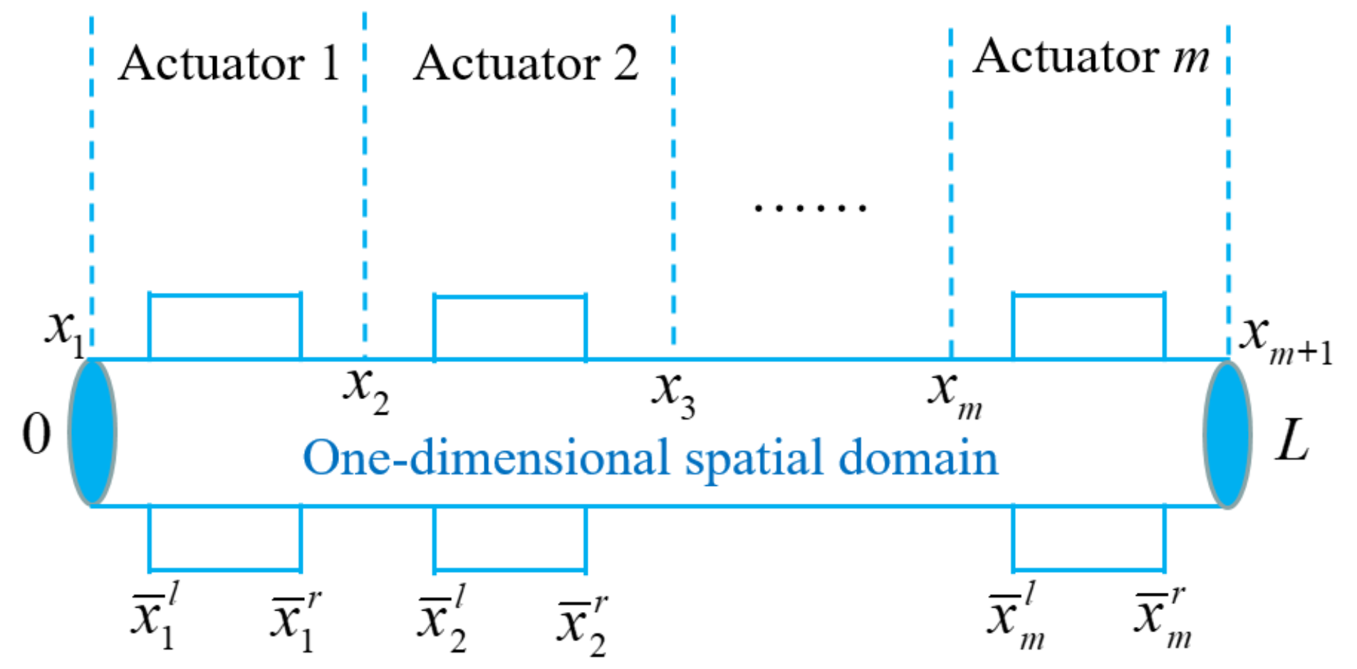
The distributions of actuators and sensors are represented by the piecewise functions, the abstract structure diagram is shown in Figure 1. It can be implemented by patch-type actuators and sensors in engineering system. The mathematical form of the distribution function is as follows
Remark 2.
Based on the distributions of actuators and sensors, the spatial domain is divided into m subdomains via spatial domain decomposition method. It can be expressed as , and should satisfy the condition . The execution positions of the actuators and sensors are within the decomposed subdomains, i.e., .
2.2. Preliminaries
For the development of this study in this paper, some essential assumption and basical lemmas are presented as follows:
Assumption 1.
The initial values of the repeatable reaction–diffusion system is equal to the initial value of the desired system for each k iteration, i.e., .
Lemma 2
(Cauchy–Schwartz Inequality for integrals). Let and be any two real integrable functions in , then the following inequality holds
Lemma 3
(Young’s inequality with ). If and are nonnegative real numbers, then the following inequality holds for any real number
3. Iterative Learning Control Design
In this section, we will present two iterative learning schemes: (1) Open-loop iterative learning scheme that the control signal is updated using the information from the previous iteration of the repetitive system. (2) Closed-loop iterative learning scheme that the control signal is updated using the information from the current iteration of the repetitive system. The objective of this paper is to make the trajectory of repeatable reaction–diffusion system (4) can track the desired trajectory using the designed iterative learning schemes.
3.1. Open-Loop P-Type Iterative Learning Control Design
Firstly, an open-loop P-type iterative learning algorithm for the repeatable reaction–diffusion system (4) with time delay is proposed. Define the i-th measurement output error between the output trajectory in the iterative process and the desired trajectory as
The open-loop learning law is designed as follows
where are the open-loop learning gains to be determined.
Define the state error and input error at the k-th iteration as follows
Applying the mean value theorem for integrals, we have the output error at the k-th iteration
where and .
Differentiate and consider the boundary condition and initial value (4), we have
subject to the Dirichlet boundary conditions and initial value
3.2. Closed-Loop P-Type Iterative Learning Control Design
Then, a closed-loop P-type iterative learning algorithm for the repeatable reaction–diffusion system (4) with time delay is proposed. The closed-loop iterative learning law is designed as follows
where are the closed-loop learning gains to be determined.
According to the definition in (14), we have the input error at the ()-th iteration
and the output error at the iteration
Differentiate and consider the boundary condition and initial value (4), we have
subject to the Dirichlet boundary conditions and initial value
4. Convergence Analysis
4.1. Open-Loop ILC Convergence Analysis
Theorem 1.
For the repeatable reaction–diffusion system (4) with time delay, α and β are konwn constants. Given suitable positive scalars and η, if there exist appropriate open-loop iterative learning gains making the following constraints safisfied:
where
in which . Then the trajectory of repeatable reaction–diffusion system (4) can track the desired trajectory using the designed iterative learning schemes (13).
Proof.
Let construct a Lyapunov–Krasovskii functional cascade in terms of time delay as follows
where
in which is an unknown constant coefficient.
Differentiate along with time t, obtaining
Based on the integration by parts technique, Poincaré–Wirtinger inequality in Lemma 1 and boundary condition in (19), it is obtained that
where .
Differentiate the Lyapunov function along with time t, we have
Substituting the time differentiation of and into the Lyapunov–Krasovskii functional cascade (27), we have
where , and
Considering the inequality (32), we can obtain for any scalar
where and is to be determined in Theorem 2.
If the LMI constraint in Theorem 1 is fulfilled, it is obtained
Integrating the inequality (34) from 0 to t and considering the initial value , we have
From the definition of in (27), the following equation holds
Multiplying both sides of the inequality (37) by , we can get
where is a constant.
From the definition of -norm in Definition 1, the inequality (38) is rewritten as
Based on Cauchy-Schwarz inequality for integrals in Lemma 2, the following inequality holds
From the derivation of in (17) and the -norm in Definition 1, we have
Then, we can obtain from (41)
where .
If is large enouth, then . From the constraint in Theorem 1 that , it is obtained . It is easily derived from (42) that
Meanwhile, from the deravation of (39), we can get
Based on the definition of -norm, it can be derived from (44) that
4.2. Closed-Loop ILC Convergence Analysis
Theorem 2.
For the repeatable reaction–diffusion system (4) with time delay, α and β are konwn constants. Given suitable positive scalars and ζ, if there exist appropriate parameter making the following constraints safisfied:
where
and the closed-loop iterative learning gain is
Proof.
Let construct a Lyapunov–Krasovskii functional cascade in terms of time delay as follows
where
where is an unknown constant coefficient.
Differentiate along with time t and consider the Poincaré–Wirtinger inequality, it is obtained
Similar to the derivation of (31), the time differentiation of Lyapunov–Krasovskii functional cascade is rewritten as
where , and
Similar to the derivation of (33), it is obtained that
where and is to be determined in Theorem 2.
If the LMI constraint in Theorem 2 is fulfilled, similar to the derivation of (34)–(36), it is obtained
Multiplying both sides of the inequality (51) by , we can get
Considering the derivation of in (23) and applying Young’s inequality in Lemma 3, we have
The inequality (53) can be rewritten as
where .
If is large enouth, then . From the constraint in Theorem 2 that , then . It is easily derived from (54) that
Then, it can be derived from (55) based on the definition of -norm
5. Numerical Simulation
In this section, we will present some numerical simulation experiments to verify the effectiveness of the proposed method. Through given some scalar parameters, the controller gains of the open-loop and closed-loop ILC can be obtained from Theorems 1 and 2. Bringing the ILC controllers into the reaction–diffusion system and operating k iterations, the trajectory of the iterative system will track the desired trajectory. Next, the simulation results of the open-loop and closed-loop ILC approaches will be addressed below, respectively.
5.1. Open-Loop ILC Simulation
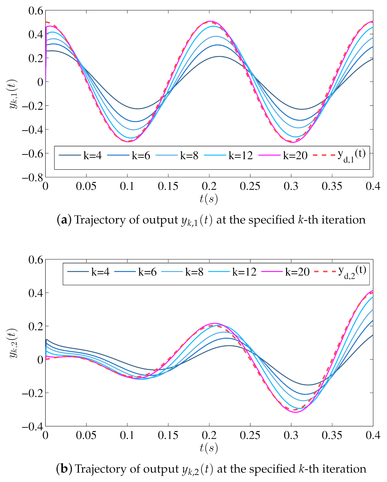
Firstly, the numerical simulation for the reaction–diffusion system (4) with time delay using open-loop iterative learning schemes (13) is presneted. The parameter settings are shown in Table 1 and there are two actuators are acting at and . By solving the LMI constraint (26) via Matlab software, we can obtain . Set , it can be calculated that , which implies . Assume the desired outs as . Then, the numerical simulation results for the reaction–diffusion system (4) with time delay using open-loop iterative learning schemes (13) are presented in the following graphics.
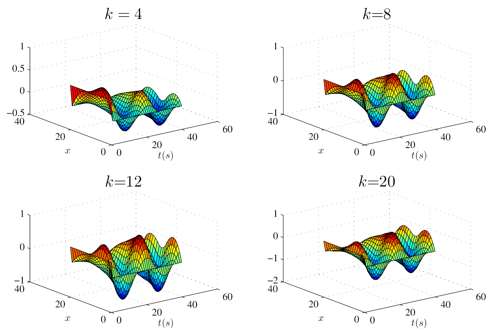
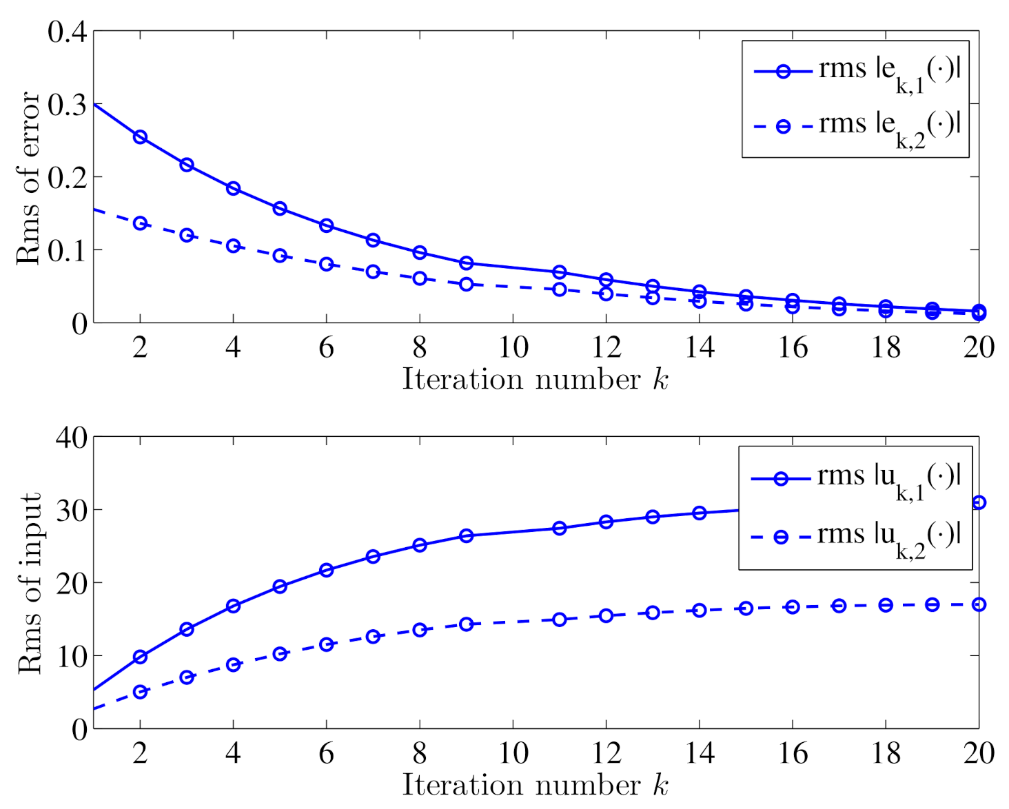
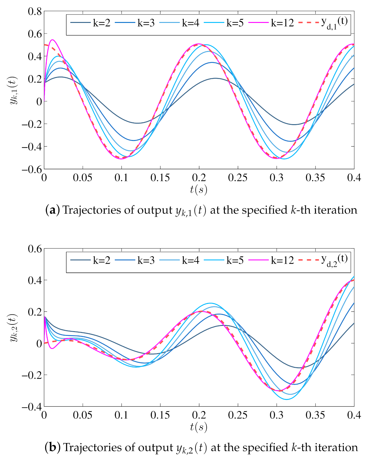
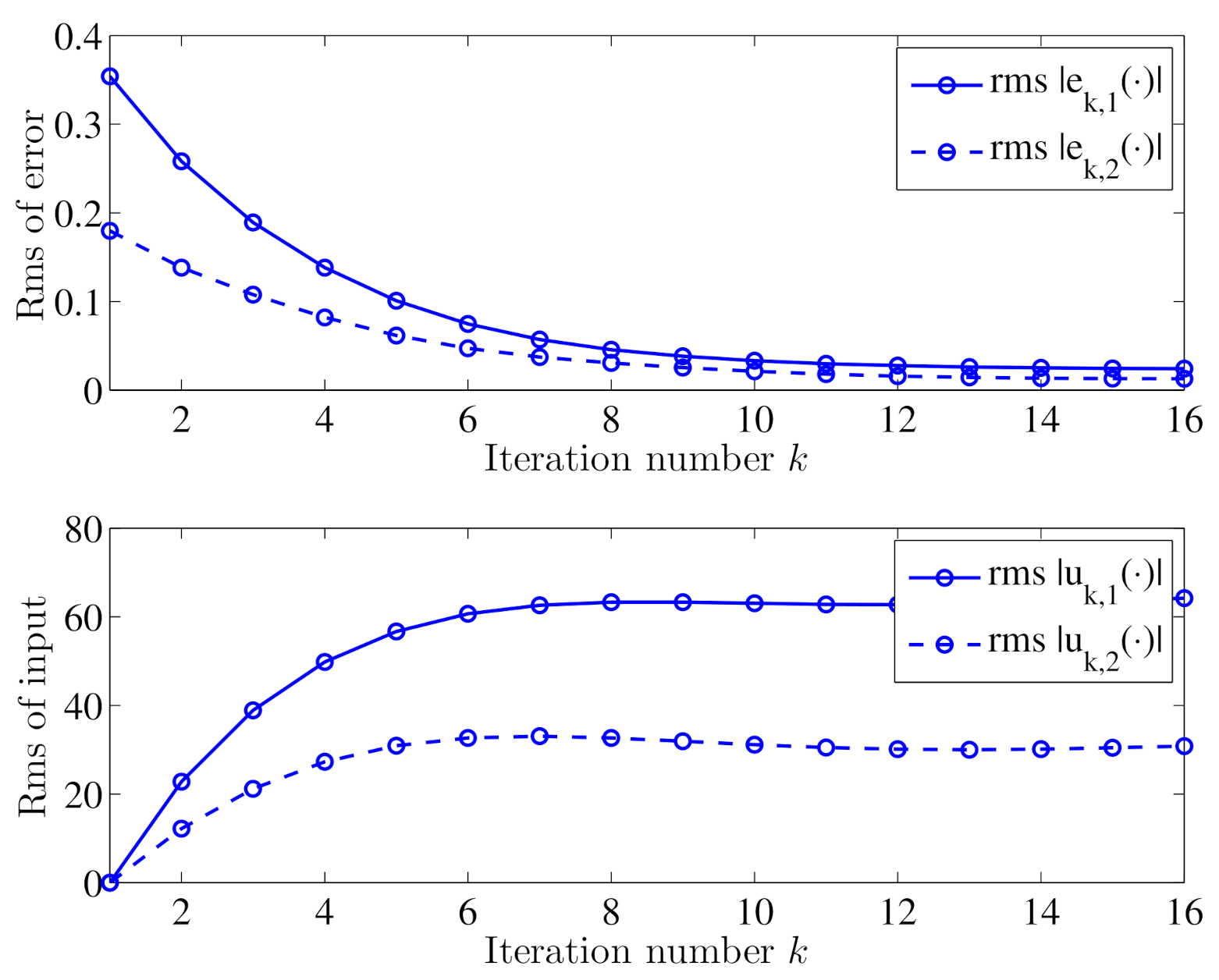
Figure 2 shows the output trajectories of in the iterative learning process marked with blue solid lines, and the desired output trajectories marked with red dotted lines. Figure 3 shows the trajectory of in the iterative learning process at several specified iterations. Figure 4 shows the trajectories of rms inputs and rms output errors in the iterative learning process. It can be seen from Figure 2 and Figure 3 that along with the number of iterations increases, the outputs will gradually track the desired trajectories , and from Figure 4 that the output errors will tend to zero and the inputs will remain unchanged. Therefore, we can conclude that the designed open-loop iterative learning schemes (13) can make the iterative process of the reaction–diffusion system (4) with time delay convergent.
5.2. Closed-Loop ILC Simulation
Then, the numerical simulation for the reaction–diffusion system (4) with time delay using closed-loop iterative learning schemes (20) is presneted. The parameter settings are shown in Table 1. By solving the LMI constraint (46) via Matlab software, we can obtain . Set , it can be calculated that , which implies . Then, the numerical simulation results for the reaction–diffusion system (4) with time delay using closed-loop iterative learning schemes (20) are presented in the following graphics.
Figure 5 shows the output trajectories of in the iterative learning process and the desired trajectories , and Figure 6 shows the trajectories of rms inputs and rms output errors in the iterative learning process. It can be seen from Figure 5 that along with the number of iterations increases, the outputs will gradually track the desired trajectories , and from Figure 6 that the output errors will tend to zero and the inputs will remain unchanged. Therefore, we can conclude that the designed closed-loop iterative learning schemes (20) can make the iterative process of the reaction–diffusion system (4) with time delay convergent. It can be easily obtained from Figure 4 and Figure 6 that the reaction–diffusion system (4) using closed-loop iterative learning approach will converge faster than the open-loop method.
6. Conclusions
This paper has presented two iterative learning schemes to deal with the trajectory tracking problem of the reaction–diffusion system. For open-loop P-type iterative learning scheme, the control signal is updated using the information from the previous iteration of the repeatable system, and for closed-loop P-type iterative learning scheme, the control signal is updated using the information from the current iteration. A new Lyapunov–Krasovskii functional is constructed to solve the time delay problem in the iterative learning process. Two theorems satisfying the sufficient conditions are provided for the convergence of the iterative learning process are proposed. Numerical simulation experiments for the open-loop and closed-loop iterative learning schemes are presented, respectively. Through numerical simulation experiments, it can be concluded that the designed iterative learning schemes can make the iterative process of the reaction–diffusion system (4) with time delay convergent. In future work, robust iterative learning control for reaction–diffusion system with input and output constraints will be studied.
Author Contributions
Conceptualization, Y.L.; methodology, Y.L.; software, J.L.; validation, Z.J.; formal analysis, Y.L.; investigation, Z.J.; resources, J.L.; data curation, J.L.; writing—original draft preparation, Y.L.; writing—review and editing, Y.L.; visualization, Z.J.; supervision, J.L.; project administration, J.L.; funding acquisition, J.L. All authors have read and agreed to the published version of the manuscript.
Funding
This research was funded by National Natural Science Foundation of China (Grant Nos. 62001127, 62003275, 62003044) and Fundamental Research Funds for the Central Universities of China (Grant No. 31020190QD039).
Institutional Review Board Statement
Not applicable.
Informed Consent Statement
Not applicable.
Data Availability Statement
Not applicable.
Conflicts of Interest
The authors declare no conflict of interest.
Abbreviations
The following abbreviations are used in this manuscript:
| ILC | Iterative Learning Control |
| PDE | Partial Differential Equation |
| D-PDE | Delay Partial Differential Equation |
| MIMO | Multiple Inputs and Multiple Outputs |
| RMS | Root Mean Square |
References
- Wu, M.; He, Y.; She, J.H.; Liu, G.P. Delay-dependent criteria for robust stability of time-varying delay systems. Automatica 2004, 40, 1435–1439. [Google Scholar] [CrossRef]
- Wu, M.; He, Y.; She, J.H. New delay-dependent stability criteria and stabilizing method for neutral systems. IEEE Trans. Autom. Control. 2004, 49, 2266–2271. [Google Scholar] [CrossRef] [Green Version]
- He, Y.; Wu, M.; She, J.H.; Liu, G.P. Delay-dependent robust stability criteria for uncertain neutral systems with mixed delays. Syst. Control Lett. 2004, 51, 57–65. [Google Scholar] [CrossRef]
- Zhang, X.M.; Wu, M.; She, J.H.; He, Y. Delay-dependent stabilization of linear systems with time-varying state and input delays. Automatica 2005, 41, 1405–1412. [Google Scholar] [CrossRef]
- Zhang, C.K.; He, Y.; Jiang, L.; Wu, M. Stability analysis for delayed neural networks considering both conservativeness and complexity. IEEE Trans. Neural Netw. Learn. Syst. 2015, 27, 1486–1501. [Google Scholar] [CrossRef] [PubMed] [Green Version]
- Lu, C.; Wu, M.; He, Y. Stubborn state estimation for delayed neural networks using saturating output errors. IEEE Trans. Neural Netw. Learn. Syst. 2019, 31, 1982–1994. [Google Scholar] [CrossRef] [PubMed]
- Lu, C.; Zhang, X.M.; Wu, M.; Han, Q.L.; He, Y. Receding horizon synchronization of delayed neural networks using a novel inequality on quadratic polynomial functions. IEEE Trans. Syst. Man Cybern. Syst. 2019, 1–11. [Google Scholar] [CrossRef]
- Lin, Z.; Fang, H. On asymptotic stabilizability of linear systems with delayed input. IEEE Trans. Autom. Control 2007, 52, 998–1013. [Google Scholar] [CrossRef]
- Zhou, B.; Lin, Z.; Duan, G. Stabilization of linear systems with input delay and saturation–a parametric Lyapunov equation approach. Int. J. Robust Nonlinear Control 2010, 20, 1502–1519. [Google Scholar] [CrossRef]
- Zhou, B.; Gao, H.; Lin, Z.; Duan, G.R. Stabilization of linear systems with distributed input delay and input saturation. Automatica 2012, 48, 712–724. [Google Scholar] [CrossRef]
- Zhang, S.; Han, W.; Zhang, Y. Finite time convergence incremental nonlinear dynamic inversion-based attitude control for flying-wing aircraft with actuator faults. Actuators 2020, 9, 70. [Google Scholar] [CrossRef]
- Tran, M.T.; Lee, D.H.; Chakir, S.; Kim, Y.B. A novel adaptive super-twisting sliding mode control scheme with time-delay estimation for a single ducted-fan unmanned aerial vehicle. Actuators 2021, 10, 54. [Google Scholar] [CrossRef]
- Liu, J.; Yu, Y.; He, H.; Sun, C. Team-triggered practical fixed-time consensus of double-integrator agents with uncertain disturbance. IEEE Trans. Cybern. 2020, 51, 3263–3272. [Google Scholar] [CrossRef] [PubMed]
- Liu, J.; Zhang, Y.; Yu, Y.; Liu, H.; Sun, C. A Zeno-Free Self-Triggered Approach to Practical Fixed-Time Consensus Tracking With Input Delay. IEEE Trans. Syst. Man Cybern. Syst. 2021, 1–11. [Google Scholar] [CrossRef]
- Roman, R.C.; Precup, R.E.; Petriu, E.M. Hybrid data-driven fuzzy active disturbance rejection control for tower crane systems. Eur. J. Control 2021, 58, 373–387. [Google Scholar] [CrossRef]
- Zhang, H.; Liu, X.; Ji, H.; Hou, Z.; Fan, L. Multi-agent-based data-driven distributed adaptive cooperative control in urban traffic signal timing. Energies 2019, 12, 1402. [Google Scholar] [CrossRef] [Green Version]
- Wang, J.W.; Wu, H.N. Some extended Wirtinger’s inequalities and distributed proportional-spatial integral control of distributed parameter systems with multi-time delays. J. Frankl. Inst. 2015, 352, 4423–4445. [Google Scholar] [CrossRef]
- Wang, J.W.; Sun, C.Y. Delay-dependent exponential stabilization for linear distributed parameter systems with time-varying delay. J. Dyn. Syst. Meas. Control 2018, 140, 051003. [Google Scholar] [CrossRef]
- Wu, H.N. Delay-dependent stability analysis and stabilization for discrete-time fuzzy systems with state delay: A fuzzy Lyapunov–Krasovskii functional approach. IEEE Trans. Syst. Man Cybern. Part B 2006, 36, 954–962. [Google Scholar]
- Wu, H.N.; Li, H.X. New approach to delay-dependent stability analysis and stabilization for continuous-time fuzzy systems with time-varying delay. IEEE Trans. Fuzzy Syst. 2007, 15, 482–493. [Google Scholar] [CrossRef]
- Wang, Z.P.; Wu, H.N. Robust guaranteed cost sampled-data fuzzy control for uncertain nonlinear time-delay systems. IEEE Trans. Syst. Man Cybern. Syst. 2017, 49, 964–975. [Google Scholar] [CrossRef]
- Wang, Z.P.; Wu, H.N.; Huang, T. Sampled-Data Fuzzy Control for Nonlinear Delayed Distributed Parameter Systems. IEEE Trans. Fuzzy Syst. 2020, 1. [Google Scholar] [CrossRef]
- Krstic, M. Delay Compensation for Nonlinear, Adaptive and PDE Systems; Spring: Berlin/Heidelberg, Germany, 2009. [Google Scholar]
- Ye, X. Adaptive stabilization of time-delay feedforward nonlinear systems. Automatica 2011, 47, 950–955. [Google Scholar] [CrossRef]
- Zhu, Y.; Krstic, M.; Su, H. Adaptive global stabilization of uncertain multi-input linear time-delay systems by PDE full-state feedback. Automatica 2018, 96, 270–279. [Google Scholar] [CrossRef]
- Zhang, H.; Pal, N.R.; Sheng, Y.; Zeng, Z. Distributed adaptive tracking synchronization for coupled reaction–diffusion neural network. IEEE Trans. Neural Netw. Learn. Syst. 2018, 30, 1462–1475. [Google Scholar] [CrossRef]
- Steeves, D.; Camacho-Solorio, L.; Benosman, M.; Krstic, M. Prescribed-time tracking for triangular systems of reaction–diffusion PDEs. IFAC-PapersOnLine 2020, 53, 7629–7634. [Google Scholar] [CrossRef]
- Nevins, T.D.; Kelley, D.H. Front tracking for quantifying advection-reaction–diffusion. Chaos Interdiscip. J. Nonlinear Sci. 2017, 27, 043105. [Google Scholar] [CrossRef] [Green Version]
- Cristofaro, A. Robust tracking control for a class of perturbed and uncertain reaction–diffusion equations. IFAC Proc. Vol. 2014, 47, 11375–11380. [Google Scholar] [CrossRef] [Green Version]
- Xu, J.X. A survey on iterative learning control for nonlinear systems. Int. J. Control 2011, 84, 1275–1294. [Google Scholar] [CrossRef]
- Bien, Z.; Xu, J.X. Iterative Learning Control: Analysis, Design, Integration and Applications; Springer Science & Business Media: Berlin/Heidelberg, Germany, 2012. [Google Scholar]
- Shen, D.; Wang, Y. Survey on stochastic iterative learning control. J. Process Control 2014, 24, 64–77. [Google Scholar] [CrossRef]
- Tayebi, A. Adaptive iterative learning control for robot manipulators. Automatica 2004, 40, 1195–1203. [Google Scholar] [CrossRef]
- Shi, J.; Xu, J.; Sun, J.; Yang, Y. Iterative Learning Control for time-varying systems subject to variable pass lengths: Application to robot manipulators. IEEE Trans. Ind. Electron. 2019, 67, 8629–8637. [Google Scholar] [CrossRef]
- Xing, X.; Liu, J. Modeling and robust adaptive iterative learning control of a vehicle-based flexible manipulator with uncertainties. Int. J. Robust Nonlinear Control 2019, 29, 2385–2405. [Google Scholar] [CrossRef]
- Dai, X.; Tian, S.; Peng, Y.; Luo, W. Closed-loop P-type iterative learning control of uncertain linear distributed parameter systems. IEEE/CAA J. Autom. Sin. 2014, 1, 267–273. [Google Scholar]
- Dai, X.S.; Tian, S.P.; Guo, Y.J. Iterative learning control for discrete parabolic distributed parameter systems. Int. J. Autom. Comput. 2015, 12, 316–322. [Google Scholar] [CrossRef] [Green Version]
- Zhang, J.; Cui, B.; Dai, X.; Jiang, Z. Iterative learning control for distributed parameter systems based on non-collocated sensors and actuators. IEEE/CAA J. Autom. Sin. 2019, 7, 865–871. [Google Scholar] [CrossRef]
- Dai, X.; Wang, C.; Tian, S.; Huang, Q. Consensus control via iterative learning for distributed parameter models multi-agent systems with time-delay. J. Frankl. Inst. 2019, 356, 5240–5259. [Google Scholar] [CrossRef]
- Zhang, J.; Cui, B.; Lou, X.Y. Iterative learning control for semi-linear distributed parameter systems based on sensor-actuator networks. IET Control Theory Appl. 2020, 14, 1785–1796. [Google Scholar] [CrossRef]
- Zhou, X.; Wang, H.; Tian, Y.; Dai, X. Iterative learning control-based tracking synchronization for linearly coupled reaction–diffusion neural networks with time delay and iteration-varying switching topology. J. Frankl. Inst. 2021, 358, 3822–3846. [Google Scholar] [CrossRef]
- He, W.; Meng, T.; Huang, D.; Li, X. Adaptive boundary iterative learning control for an Euler–Bernoulli beam system with input constraint. IEEE Trans. Neural Netw. Learn. Syst. 2017, 29, 1539–1549. [Google Scholar] [CrossRef] [PubMed]
- He, W.; Meng, T.; He, X.; Ge, S.S. Unified iterative learning control for flexible structures with input constraints. Automatica 2018, 96, 326–336. [Google Scholar] [CrossRef]
- Meng, T.; He, W. Iterative Learning Control for Flexible Structures; Springer: Berlin/Heidelberg, Germany, 2020. [Google Scholar]
- Liu, Y.Q.; Wang, J.W.; Sun, C.Y. Observer-based output feedback compensator design for linear parabolic PDEs with local piecewise control and pointwise observation in space. IET Control Theory Appl. 2018, 12, 1812–1821. [Google Scholar] [CrossRef]
- Wang, J.W.; Liu, Y.Q.; Sun, C.Y. Pointwise exponential stabilization of a linear parabolic PDE system using non-collocated pointwise observation. Automatica 2018, 93, 197–210. [Google Scholar] [CrossRef]
- Curtain Ruth, F.Z.H. An Introduction to Infinite-Dimensional Linear Systems Theory; Springer Science & Business Media: New York, NY, USA, 2012; Volume 2. [Google Scholar]
Figure 1.
Abstract structure diagram of the distributions of actuators in one-dimensional spatial domain.
Figure 1.
Abstract structure diagram of the distributions of actuators in one-dimensional spatial domain.

Figure 2.
Trajectories of outputs at the specified k-th iteration using open-loop iterative learning schemes (13).
Figure 2.
Trajectories of outputs at the specified k-th iteration using open-loop iterative learning schemes (13).

Figure 3.
Trajectories of at several specified iterations using open-loop iterative learning schemes (13).
Figure 3.
Trajectories of at several specified iterations using open-loop iterative learning schemes (13).

Figure 4.
Trajectories of inputs and output errors using open-loop iterative learning schemes (13).
Figure 4.
Trajectories of inputs and output errors using open-loop iterative learning schemes (13).

Figure 5.
Trajectories of outputs at the specified k-th iteration using closed-loop iterative learning schemes (20).
Figure 5.
Trajectories of outputs at the specified k-th iteration using closed-loop iterative learning schemes (20).

Figure 6.
Trajectories of inputs and output errors using closed-loop iterative learning schemes (20).
Figure 6.
Trajectories of inputs and output errors using closed-loop iterative learning schemes (20).


Table 1.
Parameter Settings.
| Symbol | Explanation | Value |
|---|---|---|
| L | Spatial Length | 1 |
| T | Finite Time Interval | 0.4 |
| Model Parameter | 4 | |
| Delay-Model Parameter | 1 | |
| Time Delay Parameter | 0.1 | |
| Scalar Parameter | 1 | |
| Coefficient Parameter | 0.01 | |
| p | Lyapunov Parameter | 0.6272 |
| Scalar Parameter | 0.5824 | |
| Sampling Time | 0.001s |
Publisher’s Note: MDPI stays neutral with regard to jurisdictional claims in published maps and institutional affiliations. |
© 2021 by the authors. Licensee MDPI, Basel, Switzerland. This article is an open access article distributed under the terms and conditions of the Creative Commons Attribution (CC BY) license (https://creativecommons.org/licenses/by/4.0/).
Share and Cite
MDPI and ACS Style
Liu, Y.; Li, J.; Jin, Z. Trajectory Tracking Control for Reaction–Diffusion System with Time Delay Using P-Type Iterative Learning Method. Actuators 2021, 10, 186. https://0-doi-org.brum.beds.ac.uk/10.3390/act10080186
AMA Style
Liu Y, Li J, Jin Z. Trajectory Tracking Control for Reaction–Diffusion System with Time Delay Using P-Type Iterative Learning Method. Actuators. 2021; 10(8):186. https://0-doi-org.brum.beds.ac.uk/10.3390/act10080186
Chicago/Turabian StyleLiu, Yaqiang, Jianzhong Li, and Zengwang Jin. 2021. "Trajectory Tracking Control for Reaction–Diffusion System with Time Delay Using P-Type Iterative Learning Method" Actuators 10, no. 8: 186. https://0-doi-org.brum.beds.ac.uk/10.3390/act10080186
Note that from the first issue of 2016, this journal uses article numbers instead of page numbers. See further details here.