Stabilization of Unstable Second-Order Delay Plants under PID Control: A Nyquist Curve Analysis

Abstract

Time delays arise in various components of control systems, including actuators, sensors, control algorithms, and communication links. If not properly taken into consideration, time delays will degrade the closed-loop performance and may even result in instability. This paper studies the stabilization problem of the second-order delay plants with two unstable real poles. Stabilization conditions under PD and PID control are derived using the Nyquist stability criterion. Algorithms for computing feasible PD and PID parameter regions are proposed. In some special cases, the maximal range of delay for stabilization under PD control is also given.

1. Introduction

Time delay is an inevitable phenomenon in industrial processes and natural systems due to the transmission of information and energy [1]. Delays arise either in delayed feedback control, such as in networked control systems, or naturally as a part of the dynamics within the physical process to be controlled, such as flow-temperature-composition control [1]. Even though most processes are open-loop stable, there still exist many unstable plants in chemical and biological processes, which are often more difficult to control than stable plants [2]. Often, time delay degrades the closed-loop performance of a system and leads to complications in the analysis and synthesis of the control system.

For linear time-invariant (LTI) systems with a single time delay, several methods to determine the stability by substituting the Rekasius substitution, also known as bilinear transformation, have been proposed for delay terms, by which the infinite-dimensional characteristic equation will reduce to a polynomial equation with a pseudo delay [3]. In [4], Walton and Marshall found that the introduction of a pseudo delay is unnecessary. In [5], a stability criterion was obtained via the argument principle, or via the Mikhaylov stability criterion, for retarded time delay systems. Applying the argument principle to the feedback control system with the knowledge of open-loop frequency response results in the popular Nyquist stability criterion. Meanwhile, for cases with two delays, the Cluster Treatment of Characteristic Roots (CTCR) method [6] and geometry-based methods [7,8] were proposed to obtain a complete stability map characterizing the boundary of the stable region. Note that the CTCR method and geometry-based methods share some similarities with the D-decomposition approach [9].

For the stabilization of time delay systems, the well-known Ziegler–Nichols step response method provided rules for tuning controller parameters based on the features of the step response of an open-loop stable plant. Reference [10] proposed a Ziegler–Nichols-type controller for a first-order unstable plant with a time delay. Vanavil et al. provided a direct synthesis method for a general unstable second-order plant by means of substituting $Pad\acute{e}$ approximation [11]. In [12], Tan et al. proposed an IMC-based method for both first-order and second-order unstable plants. Furthermore, for second-order delay plants with two unstable poles, stabilization was achieved based on approximation methods in [12,13]. Additionally, the pole placement method is widely used to obtain the desired closed-loop performance [14,15,16,17,18,19].

The computation for the feasible parameter region of PID control was investigated by Silva et al. for general first-order plants based on the Hermite–Biehler theorem [20]. Inspired by [20], Yu et al. considered the consensus of the multi-agent system with a first-order dynamic model and input delay [21]. Based on an extension of the Hermite–Biehler theorem, a new simple algorithm for determining the feasible parameter region has been proposed [22]. The algorithm is not only applicable to both stable and unstable systems, but can also be utilized for systems with real or complex poles. Hwang applied the D-decomposition approach to stabilize unstable first-order delay plants under PID control and constructed the complete set of stabilizing PID controller parameters [23]. In [24], Zalluhoglu et al. utilized the CTCR method and obtained the stable region in the space of the control parameter. Based on the Nyquist stability criterion, Lee et al. investigated the stabilization of a class of unstable all-pole delay plants of arbitrary order with a unstable pole and provided the maximum allowable time delay [25]. In addition, the procedures to determine the feasible PID control parameter region of a class of unstable all-pole delay plants is also given.

Robustness issues concerning uncertain delay systems have also been heavily studied. In these studies, the delay margin (DM) problem has attracted considerable interest. Middleton and Miller studied the delay margin of unstable plants achievable by LTI controllers and gave several explicit upper bounds on the achievable delay margin [26]. In [27,28,29], Ma et al. analyzed the delay margin achievable by PID controllers and proposed a computational approach. A graphical method to tune a PI/PID controller for time delay systems was presented using dominant pole placement with a specified gain margin (GM) and phase margin (PM) [30]. Extensions of problems on the robust consensus of second-order multi-agent systems were also studied; see, e.g., [31].

Due to the approximate substitution for the delay term, the method proposed in [11,12,13] is inadequately accurate. In contrast, the accurate approaches proposed in [20,21,22,23,24] are mathematically involved and do not provide an explicit characterization of the boundary of the feasible PID parameter region. Different from the previous works, we adopt the Nyquist curve analysis approach to achieve the feasible PID control parameter region, which provides an exact and explicit region and needs no complicated derivation. We focus on the stabilization of second-order delay plants with two unstable real poles under PD and PID control. A necessary and sufficient condition on the stabilization of the system under PD control is proposed. Furthermore, the corresponding algorithm to achieve the feasible PD control parameter region for the fixed delay is given. The Nyquist curve analysis approach can be also extended to the PID control scenario. Finally, two simulation results show the effectiveness of our theoretical results. Additionally, the simulation result also indicates that the role of integral control is negative to improve the feasible PID control parameter region for time delay systems.

The rest of this paper is organized as follows. In Section 2, preliminaries on stability analysis are presented and the problem formulation is given. In Section 3, the stabilizability of a second-order delay plant with two unstable real poles under PD control is investigated. A necessary and sufficient condition on the stabilization is given based on the Nyquist stability criterion. In Section 4, the stabilizability of second-order delay plants with two unstable real poles under PID control is also studied. Furthermore, algorithms for computing the feasible PD/PID control parameter region are presented. Examples are provided to illustrate the validity of the proposed algorithms in Section 5. Section 6 concludes this paper.

2. Preliminaries and Problem Formulation

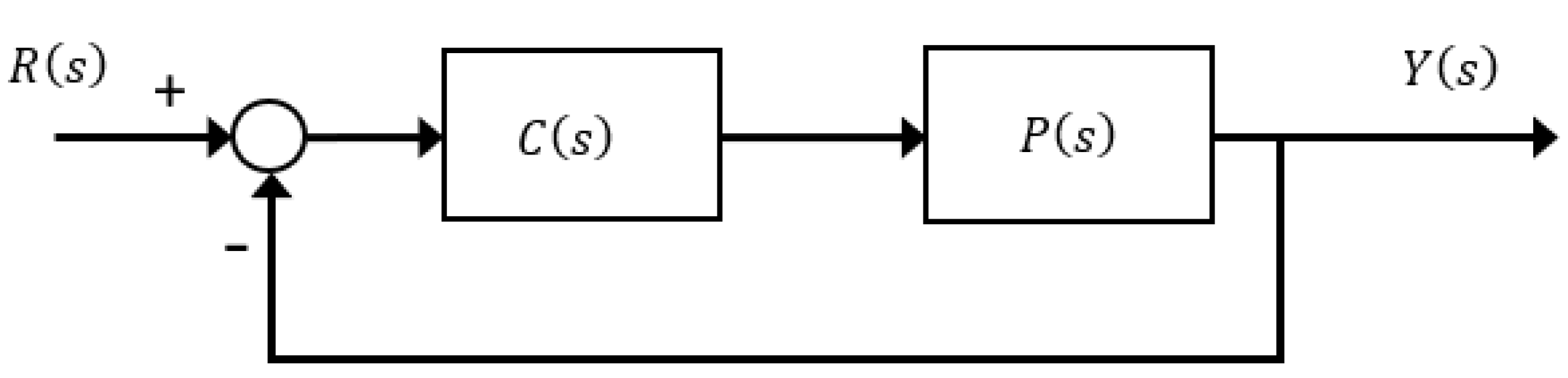
Consider a single-loop feedback control system shown in Figure 1, whose closed-loop transfer function is given by

$$\frac{Y\left(s\right)}{R\left(s\right)}=\frac{C\left(s\right)P\left(s\right)}{1+C\left(s\right)P\left(s\right)},$$

(1)

where $C\left(s\right)$ is the LTI controller, $P\left(s\right)$ is the controlled plant, $R\left(s\right)$ is the reference signal and $Y\left(s\right)$ is the output signal.

Denote the characteristic equation of the system (Equation (1)) by

$$F\left(s\right)=1+C\left(s\right)P\left(s\right)=0,$$

(2)

and the open-loop transfer function by

$$Q\left(s\right)=C\left(s\right)P\left(s\right).$$

(3)

It is well-known that the closed-loop system (Equation (1)) is stable if and only if all roots of the characteristic equation $F\left(s\right)=0$ lie in the open left-half s-plane. It is also well-known that the closed-loop stability can be ascertained by analyzing the open-loop transfer function $Q\left(s\right)$ using the graphical Nyquist stability criterion. A simplified Nyquist stability criterion is given below.

Lemma 1

([32]).For the system shown in Figure 1, if the open-loop transfer function $Q\left(s\right)=C\left(s\right)P\left(s\right)$ has N poles in the closed right-half s-plane and then for stability, the $Q\left(j\omega \right)$ locus, as ω varies from $-\infty$ to $+\infty$ and encircles the origin clockwise, must encircle the critical point, $-1+j0$, N times in the counterclockwise direction.

Lemma 2

([33]).Given the open-loop transfer function $Q\left(s\right)=C\left(s\right)P\left(s\right)$,

$$\underset{\omega \to \infty }{lim}\left|Q\left(j\omega \right)\right|<1$$

(4)

is a necessary condition for the closed-loop stability of the system shown in Figure 1.

The Nyquist stability criterion can be extended to study LTI delay systems satisfying Equation (4). Consider a second-order plant with time delay, whose transfer function is given by

$$P\left(s\right)=\frac{1}{s^2+as+b}{e}^{-\tau s},$$

(5)

where $\tau$ is a constant time delay and a, b are constant coefficients. The plant (Equation (5)) has two unstable poles if $a\le 0$ and $b\ge 0$. Specially, for the plant (Equation (5)) with two unstable real poles, there exist the following three cases:

• For $a=0$ and $b=0$, the plant (Equation (5)) is unstable with two poles at the origin;
• For $a<0$ and $b=0$, the plant (Equation (5)) is unstable with one pole at the origin and another on the positive real axis;
• For $a<0$ and $0<b\le \frac{a^2}{4}$, the plant (Equation (5)) is unstable with two poles on the positive real axis.

Under these circumstances, the plant (Equation (5)) becomes

$$P\left(s\right)=\frac{1}{(s-p_1)(s-p_2)}{e}^{-\tau s},p_1,p_2\ge 0$$

(6)

where $p_1$, $p_2$ are the two real poles. Furthermore, the constant coefficients $a,b$ of Equation (5) can be rewritten as $a=-p_1-p_2$ and $b=p_1{p}_2$.

In this paper, the low-order LTI controller considered is the PID controller

$$C_{pid}\left(s\right)=k_p+\frac{k_i}{s}+k_{d}s,$$

(7)

where $k_p,k_i,k_d$ represent proportional, integral and differential gains, respectively. The special cases of Equation (7), P, PI and PD controllers are given by

$$C_p\left(s\right)=k_p,$$

(8)

$$C_{pi}\left(s\right)=k_p+\frac{k_i}{s},$$

(9)

$$C_{pd}\left(s\right)=k_p+k_{d}s.$$

(10)

Combining Equations (5) and (7), we have the open-loop frequency response

$$Q_{pid}\left(j\omega \right)=\frac{k_p+\frac{k_i}{j\omega }+j{k}_d\omega }{b-{\omega }^2+ja\omega }{e}^{-j\tau \omega }.$$

(11)

It is clear that

$$\underset{\omega \to \infty }{lim}\left|Q_{pid}\left(j\omega \right)\right|<1.$$

The magnitude and phase of $Q_{pid}\left(j\omega \right)$ are denoted by

$$L_{pid}\left(\omega \right)=k_p\sqrt{\frac{1+{\left(\frac{k_d}{k_p}\omega -\frac{k_i}{k_p\omega }\right)}^2}{{\left(b-{\omega }^2\right)}^2+ \left(a^2{\omega }^2\right)}},$$

(12)

and

$${\mathsf{\Phi }}_{pid}\left(\omega \right)=-\tau \omega +arctan\left(\frac{k_d}{k_p}\omega -\frac{k_i}{k_p\omega }\right)+{\varphi }_1\left(\omega \right),$$

(13)

where

$${\varphi }_1\left(\omega \right)=\left\{\begin{array}{cc}arctan\frac{-a\omega }{b-{\omega }^2},\hfill & \omega <\sqrt{b},\hfill \\ \frac{\pi }{2},\hfill & \omega =\sqrt{b},\hfill \\ arctan\frac{-a\omega }{b-{\omega }^2}+\pi ,\hfill & \omega >\sqrt{b}.\hfill \end{array}\right.$$

(14)

Remark 1.

The phase ${\varphi }_1\left(\omega \right)$ is continuous at $\omega =\sqrt{b}$. As stated above, $a=-p_1-p_2\le 0$, $b=p_1{p}_2\ge 0$. For ${\varphi }_1\left(\omega \right)$ at $\omega =\sqrt{b}-0^{+}$, it follows that $b-{\omega }^2>0$ and then ${\varphi }_1\left(\omega \right)=\frac{\pi }{2}-0^{+}$. For $\omega =\sqrt{b}+0^{+}$, it follows that $b-{\omega }^2<0$ and then ${\varphi }_1\left(\omega \right)=\frac{\pi }{2}+0^{+}$. As such, the phase ${\varphi }_1\left(\omega \right)$ is continuous for any $\omega \in \left(0,+\infty \right)$. As ω varies from 0 to $+\infty$, ${\varphi }_1\left(\omega \right)$ varies from 0 to π monotonically. The conclusion can be also drawn since ${\varphi }_1\left(\omega \right)$ is rewritten as

$${\varphi }_1\left(\omega \right)=arctan\frac{\omega }{p_1}+arctan\frac{\omega }{p_2}.$$

We assume that the PID gains $k_p,k_i,k_d$ are positive throughout this paper. As such, the open-loop Nyquist curve must encircle the critical point $-1+j0$ two times anticlockwise.

In the syntheses of time delay systems, the general Nyquist stability criterion can only be used to test the stability of systems with fixed parameters. To obtain the feasible control parameter region for plants with fixed model parameters, some more specific conditions may be useful.

3. Stabilization of Delay Plants with Two Real Poles under PD Control

In this section, we focus on the stabilization of second-order delay plants with two real unstable poles under PD control. First, we discuss the stabilization problem by analyzing the open-loop frequency response of Equation (6) under PD control and propose a necessary and sufficient condition on stabilization for fixed PD control parameters. Next, the maximal delay values of two special cases are obtained by applying the necessary and sufficient condition. Finally, for given parameters $p_1, p_2\mathrm{and}\tau$, an algorithm for the computation of the stabilizing PD control parameter region is proposed.

The plant (Equation (5)) with $a<0$ and $0<b\le \frac{a^2}{4}$ is equivalent to the plant (Equation (6)) with $p_1>0$ and $p_2>0$.

It is obvious that the plant (Equation (6)) with two unstable real poles cannot be stabilized by P and PI control in light of the Nyquist stability criterion. Hence, let us consider PD control. Under the PD controller (Equation (10)), the magnitude and phase of the open-loop frequency response can be rewritten as

$$L_{pd}\left(\omega \right)=\sqrt{\frac{k_p^2+k_d^2{\omega }^2}{\left(p_1^2+{\omega }^2\right)\left(p_2^2+{\omega }^2\right)}},$$

(15)

and

$${\mathsf{\Phi }}_{pd}\left(\omega \right)=-\tau \omega +arctan\frac{k_d}{k_p}\omega +arctan\frac{\omega }{p_1}+arctan\frac{\omega }{p_2}.$$

(16)

3.1. A Necessary and Sufficient Condition for Stabilization by Fixed PD Parameters

The following theorem provides a necessary and sufficient condition for the stabilization of the plant (Equation (6)) with $p_1>0,p_2>0$ by PD control.

Theorem 1.

Let the plant be given by Equation (6). Then, the PD controller (Equation (10)) can stabilize the plant if and only if

$$max\left\{{\mathsf{\Phi }}_{pd}\left(\omega \right)\right\}>\pi ,$$

(17)

$${\omega }_s<{\omega }_{c2},$$

(18)

and

$$L_{pd}\left({\omega }_{c1}\right)>1>L_{pd}\left({\omega }_{c2}\right)$$

(19)

hold, where ${\omega }_{c1},{\omega }_{c2}$ are the frequencies satisfying ${\mathsf{\Phi }}_{pd}\left(\omega \right)=\pi$, ${\omega }_s$ is the extreme point of $L_{pd}\left(\omega \right)$ over $\omega \in \left[0,+\infty \right)$ denoted by

$${\omega }_s^2=\left\{\begin{array}{cc}0,\hfill & \mathrm{for}{k}_p^2\left(p_1^2+p_2^2\right)-k_d^2{p}_1^2{p}_2^2\ge 0,\hfill \\ \frac{-k_p^2+\sqrt{k_p^4-k_d^2\left[k_p^2(p_1^2+p_2^2)-k_d^2{p}_1^2{p}_2^2\right]}}{k_d^2},\hfill & \mathrm{for}{k}_p^2\left(p_1^2+p_2^2\right)-k_d^2{p}_1^2{p}_2^2<0.\hfill \end{array}\right.$$

(20)

Proof. 

Necessity. It is clear that $\frac{d^2{\mathsf{\Phi }}_{pd}\left(\omega \right)}{d{\omega }^2}<0$. By taking the derivative of Equation (16) with respect to $\omega$, we have

$${\left.\frac{d{\mathsf{\Phi }}_{pd}}{d\omega }\right|}_{\omega =0}=-\tau +\frac{k_d}{k_p}+\frac{1}{p_2}+\frac{1}{p_2}.$$

(21)

If $-\tau +\frac{1}{p_1}+\frac{1}{p_2}\le 0$, then ${\mathsf{\Phi }}_{pd}\left(\omega \right)$ decreases monotonically as $\omega$ varies from 0 to $+\infty$. It follows that the corresponding Nyquist curve encircles the origin clockwise, which violates the stabilization.

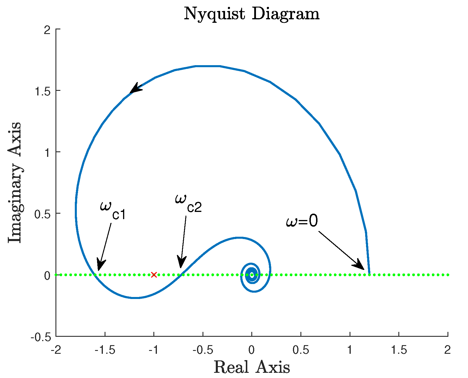
If $-\tau +\frac{1}{p_1}+\frac{1}{p_2}>0$, then ${\mathsf{\Phi }}_{pd}\left(\omega \right)$ increases monotonically as $\omega$ varies from 0 to ${\omega }_1$ and decreases monotonically as $\omega$ varies from ${\omega }_1$ to $+\infty$. To ensure the two-times anticlockwise encirclements, it is necessary that $max\left\{{\mathsf{\Phi }}_{pd}\left(\omega \right)\right\}>\pi$ or equivalently ${\mathsf{\Phi }}_{pd}\left({\omega }_1\right)>\pi$. ${\omega }_1$ is the extreme point of ${\mathsf{\Phi }}_{pd}\left(\omega \right)$.

As for the magnitude $L_{pd}\left(\omega \right)$, there exist infinite intersections between the Nyquist curve and the negative real axis, whose frequencies satisfy

$$0<{\omega }_{c1}<{\omega }_{c2}<\cdots <{\omega }_{cq}<\cdots ,$$

(22)

with

$${\mathsf{\Phi }}_{pd}\left({\omega }_{ci}\right)\left\{\begin{array}{cc}=\pi ,\hfill & \mathrm{for}i=1,2,\hfill \\ <0,\hfill & \mathrm{for}i\ge 3.\hfill \end{array}\right.$$

(23)

To ensure the stability, it is necessary that the magnitude $L_{pd}\left(\omega \right)$ satisfies

$$L_{pd}\left({\omega }_{ci}\right)\left\{\begin{array}{cc}>1,\hfill & \mathrm{for}i=1,\hfill \\ <1,\hfill & \mathrm{for}i\ge 2.\hfill \end{array}\right.$$

(24)

Figure 2 shows the tendency of the frequency response explicitly.

Next, by taking the derivative of $L_{pd}^2\left(\omega \right)$ along $\omega$, it is easy to obtain

$$\frac{d{L}_{pd}^2\left(\omega \right)}{d\omega }=\frac{-2\omega }{{\Delta }^2}\left[k_d^2{\omega }^4+2k_p^2{\omega }^2+k_p^2\left(p_1^2+p_2^2\right)-k_d^2{p}_1^2{p}_2^2\right],$$

(25)

where $\Delta =\left(p_1^2+{\omega }^2\right)\left(p_2^2+{\omega }^2\right)$. It is easy to find that if $k_p^2\left(p_1^2+p_2^2\right)-k_d^2{p}_1^2{p}_2^2>0$, then the magnitude $L_{pd}\left(\omega \right)$ decreases monotonically as $\omega$ varies from 0 to $+\infty$; otherwise, $L_{pd}\left(\omega \right)$ increases monotonically as $\omega$ varies from 0 to ${\omega }_s$ and then decreases as $\omega$ varies from ${\omega }_s$ to $+\infty$. Note that ${\omega }_s$ is the extreme point of $L_{pd}\left(\omega \right)$ over $\omega \in \left[0,+\infty \right)$, and its explicit expression is given by Equation (20).

If ${\omega }_s\ge {\omega }_{c2}$, then $L_{pd}\left({\omega }_{c1}\right)<L_{pd}\left({\omega }_{c2}\right)$, which never generates two-times anticlockwise encirclements. If both ${\omega }_s<{\omega }_{c2}$ and $\frac{L_{pd}\left({\omega }_{c1}\right)}{k_p}>\frac{L_{pd}\left({\omega }_{c2}\right)}{k_p}$ hold, we only need to choose $k_p$ appropriately to satisfy Equation (19). In addition, $\frac{L_{pd}\left({\omega }_{c1}\right)}{k_p}>\frac{L_{pd}\left({\omega }_{c2}\right)}{k_p}$ implies that ${\omega }_s<{\omega }_{c2}$.

Sufficiency. According to the above analysis on the monotonicity of magnitude and phase, if Equations (17)–(19) hold, then the corresponding Nyquist curve is shown in Figure 2. This ensures the stabilization of the plant (Equation (6)) with $p_1>0,p_2>0$ under PD control, which completes the proof. □

In the above analysis, only the case that plant (Equation (6)) with $p_1>0$ and $p_2>0$ is taken into consideration. In what follows, the plant (Equation (6)) with $p_1=0$ or/and $p_2=0$ will be analyzed for the completeness of the proof.

Specifically, if $a<0$ and $b=0$, i.e., when one pole approaches the origin, we have

$$P_{}\left(s\right)=\frac{1}{s(s-p_1)}{e}^{-\tau s},p_1>0.$$

(26)

In this case, the magnitude and phase of the open-loop frequency response become

$$L_{pd}\left(\omega \right)=\sqrt{\frac{k_d^2+\frac{k_p^2}{{\omega }^2}}{{\omega }^2+p_1^2}},$$

(27)

and

$${\mathsf{\Phi }}_{pd}\left(\omega \right)=-\tau \omega +arctan\frac{k_d\omega }{k_p}+arctan\frac{\omega }{p_1}+\frac{\pi }{2}.$$

(28)

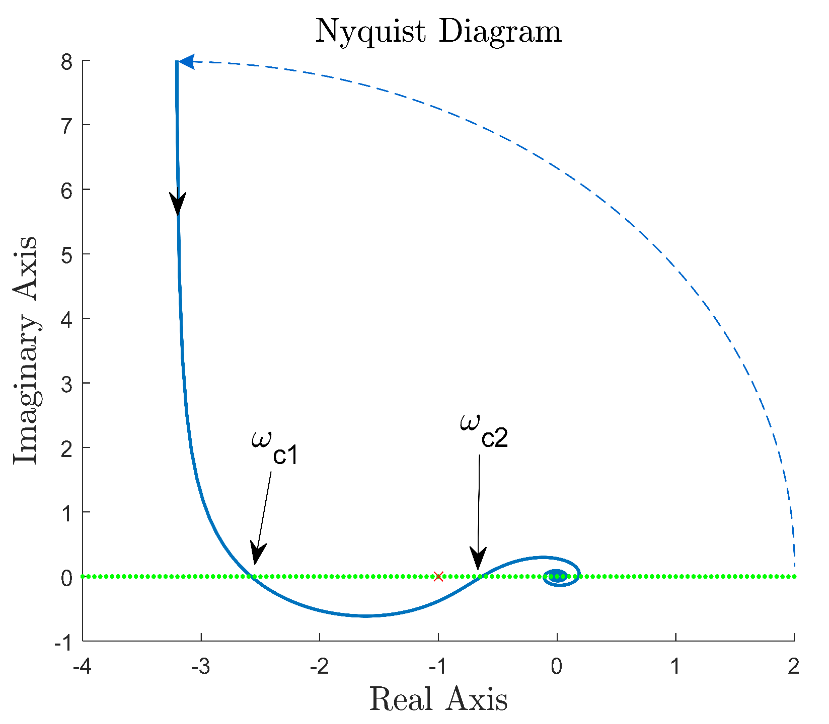
It is clear that $L_{pd}\left(\omega \right)$ decreases monotonically as $\omega$ varies from $0_{+}$ to $+\infty$. When it comes to the phase, if $-\tau +\frac{k_d}{k_p}+\frac{1}{p_1}\le 0$, then ${\mathsf{\Phi }}_{pd}\left(\omega \right)$ decreases monotonically over $\omega >0$, which violates the stability condition. To ensure the stability of the closed-loop system (Equation (1)), the ideal Nyquist curve is given by Figure 3, where ${\omega }_{c1}$ and ${\omega }_{c2}$ are the two frequencies satisfying ${\mathsf{\Phi }}_{pd}\left(\omega \right)=\pi$. In other words, Theorem 1 can be applied to the plant (Equation (26)).

Furthermore, the upper bound of time delay $\tau$ for the stabilization of the plant (Equation (26)) under PD control is given by the corollary below.

Corollary 1.

Let the plant be given by Equation (26). There exists a PD controller (Equation (10)) to stabilize the plant if and only if

$$\tau <\frac{1}{p_1}.$$

(29)

Proof. 

It is clear that $L_{pd}\left(\omega \right)$ decreases monotonically as $\omega$ varies from $0_{+}$ to $+\infty$. It follows that ${\omega }_s=0$. If $\max \left\{{\mathsf{\Phi }}_{pd}\left(\omega \right)\right\}>\pi$, there must exist some $k_p$ such that $L_{pd}\left({\omega }_{c1}\right)>1>L_{pd}\left({\omega }_{c2}\right)$. There exists a PD controller (Equation (10)) to stabilize the plant (Equation (26)) if and only if $\max \left\{{\mathsf{\Phi }}_{pd}\left(\omega \right)\right\}>\pi$. Suppose that the extreme point of ${\mathsf{\Phi }}_{pd}\left(\omega \right)$ is ${\omega }_1$. For Equation (28), $\max \left\{{\mathsf{\Phi }}_{pd}\left(\omega \right)\right\}>\pi$ can be transformed into

$$-\tau {\omega }_1+arctan\frac{k_d{\omega }_1}{k_p}+arctan\frac{{\omega }_1}{p_1}>\frac{\pi }{2}.$$

(30)

In Equation (30), $arctan\frac{k_d{\omega }_1}{k_p}<\frac{\pi }{2}$, it follows that $-\tau {\omega }_1+arctan\frac{{\omega }_1}{p_1}>0$. Furthermore, $-\tau {\omega }_1+\frac{{\omega }_1}{p_1}>-\tau {\omega }_1+arctan\frac{{\omega }_1}{p_1}>0$. It is clear that if $\max \left\{{\mathsf{\Phi }}_{pd}\left(\omega \right)\right\}>\pi$ holds, $\tau$ should be less than $\frac{1}{p_1}$. In Equation (28), if $\tau <\frac{1}{p_1}$, there must exist a sufficiently large $\frac{k_d}{k_p}$ such that $\max \left\{{\mathsf{\Phi }}_{pd}\left(\omega \right)\right\}>\pi$. It follows that $\max \left\{{\mathsf{\Phi }}_{pd}\left(\omega \right)\right\}>\pi$ holds if and only if $\tau <\frac{1}{p_1}$.

In other words, there exists a PD controller (Equation (10)) to stabilize the plant (Equation (26)) if and only if $\tau <\frac{1}{p_1}$. □

More specifically, if $a=0$ and $b=0$, which corresponds to the plant with two poles located at the origin, i.e.,

$$P_{}\left(s\right)=\frac{1}{s^2}{e}^{-\tau s}.$$

(31)

Then, under the PD controller (Equation (10)), the magnitude and phase of the open-loop frequency response become

$$L_{pd}\left(\omega \right)=\sqrt{\frac{k_d^2+\frac{k_p^2}{{\omega }^2}}{{\omega }^2}}$$

(32)

and

$${\mathsf{\Phi }}_{pd}\left(\omega \right)=-\tau \omega +arctan\frac{k_d\omega }{k_p}+\pi .$$

(33)

It is clear that $L_{pd}\left(\omega \right)$ decreases monotonically as $\omega$ varies from $0_{+}$ to $+\infty$. When it comes to the phase, if $-\tau +\frac{k_d}{k_p}\le 0$, then ${\mathsf{\Phi }}_{pd}\left(\omega \right)$ decreases monotonically without anticlockwise intersection of the Nyquist curve and negative real axis, which violates the stability. To ensure the stability of the closed-loop system (Equation (1)), the Nyquist curve is shown in Figure 4.

Corollary 2.

Let $P\left(s\right)$ be given by Equation (31). There exists a PD controller (Equation (10)) to stabilize the plant (Equation (31)) for an infinite time delay τ.

Proof. 

It is clear that $L_{pd}\left(\omega \right)$ decreases monotonically as $\omega$ varies from $0_{+}$ to $+\infty$. It follows that ${\omega }_s=0$. If $\max \left\{{\mathsf{\Phi }}_{pd}\left(\omega \right)\right\}>\pi$, there must exist some $k_p$ such that $L_{pd}\left({\omega }_{c1}\right)>1>L_{pd}\left({\omega }_{c2}\right)$. There exists a PD controller (Equation (10)) to stabilize the plant (Equation (31)) if and only if $\max \left\{{\mathsf{\Phi }}_{pd}\left(\omega \right)\right\}>\pi$. Suppose that the extreme point of ${\mathsf{\Phi }}_{pd}\left(\omega \right)$ is ${\omega }_1$. For Equation (33), $\max \left\{{\mathsf{\Phi }}_{pd}\left(\omega \right)\right\}>\pi$ can be transformed into

$$-\tau {\omega }_1+arctan\frac{k_d{\omega }_1}{k_p}>0.$$

(34)

In Equation (34), there must exist a sufficiently large $\frac{k_d}{k_p}>\tau$ such that $\max \left\{{\mathsf{\Phi }}_{pd}\left(\omega \right)\right\}>\pi$. In other words, there exists a PD controller (Equation (10)) to stabilize the plant (Equation (31)) with an infinite time delay $\tau$. □

It is worth noting that, inspired by [27], for fixed $\tau$, $p_1$ and $p_2$, we can also obtain the feasible PD control parameter region in view of the following inequality:

$$-\tau {\omega }_c+arctan\frac{k_d{\omega }_c}{k_p}+arctan\frac{{\omega }_c}{p_1}+arctan\frac{{\omega }_c}{p_2}>\pi ,$$

(35)

where ${\omega }_c$ is the ultimate frequency. The following section will describe how to achieve the region through an algorithm.

3.2. An Algorithm for Feasible Parameter Region of PD Control

Based on the Nyquist stability criterion, Theorem 1 gives the stabilization condition for fixed $k_p$ and $k_d$. Furthermore, we have some observations: (i) if we increase $\frac{k_d}{k_p}$ to keep the necessary condition (Equation (17)), the extreme point ${\omega }_s$ of $L_{pd}\left(\omega \right)$ may increase, then $L_{pd}\left({\omega }_{c1}\right)<L_{pd}\left({\omega }_{c1}\right)$. This will never stabilize the system. (ii) The proportional gain $k_p$ only affects the magnitude $L_{pd}\left(\omega \right)$. Therefore, to stabilize the plant (Equation (6)) by PD control, we only need to choose $\frac{k_d}{k_p}$ appropriately to satisfy the phase condition (Equation (17)) and the magnitude condition

$$\frac{L_{pd}\left({\omega }_{c1}\right)}{k_p}>\frac{L_{pd}\left({\omega }_{ci}\right)}{k_p},i\ge 2.$$

(36)

If such $\frac{k_d}{k_p}$ does not exist, it follows that the plant (Equation (6)) cannot be stabilized by PD control. Otherwise, we choose $k_p$ appropriately to satisfy the magnitude condition (Equation (24)). Finally, the stabilizing PD controller can be designed accordingly.

Algorithm 1 for computing the PD parameter region of the plant (Equation (6)) is shown as follows:

Algorithm 1 The algorithm for the feasible PID parameter region of the plant (6).

Step 1: Compute the maximal value of $-\tau \omega +arctan\frac{\omega }{p_1}+arctan\frac{\omega }{p_2}$. If the maximum is less than $\frac{\pi }{2}$, then the plant cannot be stabilized due to the overlarge $\tau$. Step 2: For fixed $\tau$, determine the lower bound and upper bound of the range $\frac{k_d}{k_p}\in \left[\underline{d},\overline{d}\right]$. $\overline{d}$ is initialized by a sufficiently large positive value. $\underline{d}$ is the smallest $\frac{k_d}{k_p}\in \left[0,\overline{d}\right]$, which satisfies $\max \left\{{\mathsf{\Phi }}_{pd}\left(\omega \right)\right\}>\pi$. Step 3: Select a $\frac{k_d}{k_p}$ in the range $\left[\underline{d},\overline{d}\right]$ and solve ${\omega }_{c1},{\omega }_{c1}$ from ${\mathsf{\Phi }}_{pd}\left(\omega \right)=\pi$. Step 4: Compute the lower bound and upper bound of $k_p$ by $\underline{k_p}=\frac{1}{L_{pd}\left({\omega }_{c1}\right)/k_p}$, $\overline{k_p}=\frac{1}{L_{pd}\left({\omega }_{c2}\right)/k_p}$. Step 5: By sweeping over $\frac{k_d}{k_p}$ in the range $\left[\underline{d},\overline{d}\right]$, repeat Steps 3–4 to obtain the complete feasible parameter region of PD controllers.

Remark 2.

For the plants (Equations (26) and (31)), Algorithm 1 is not necessary. For Equation (26), it is easy to determine its stabilizability under PD control by comparing τ and $\frac{1}{p_1}$. For Equation (31), it is unnecessary to verify its stabilizability under PD control according to Corollary 2. In addition, the frequency of the first intersection between the Nyquist curve and negative real axis, ${\omega }_{c1}$, is an infinitesimal positive value. It is obvious that the magnitude of the first intersection is $+\infty$, which implies that $L_{pd}\left({\omega }_{c1}\right)>1$.

4. Stabilization of Delay Plants with Two Unstable Real Poles under PID Control

4.1. A Sufficient Condition for Stabilization by Fixed PID Parameters

In what follows, we consider the stabilization of the plant (Equation (6)) under the PID controller (Equation (7)). The corresponding magnitude and phase of the open-loop frequency response can be rewritten as

$$L_{pid}\left(\omega \right)=\sqrt{\frac{k_p^2+{(k_d\omega -\frac{k_i}{\omega })}^2}{\left(p_1^2+{\omega }^2\right)\left(p_2^2+{\omega }^2\right)}},$$

(37)

and

$${\mathsf{\Phi }}_{pid}\left(\omega \right)=-\tau \omega +arctan\frac{\omega }{p_1}+arctan\frac{\omega }{p_2}+{\varphi }_2\left(\omega \right),$$

(38)

where

$${\varphi }_2\left(\omega \right)=arctan\left(\frac{k_d}{k_p}\omega -\frac{k_i}{k_p\omega }\right).$$

(39)

The equivalence between Equations (12), (13), (37) and (38) can be ascertained by substituting $a=-p_1-p_2\le 0$, $b=p_1{p}_2\ge 0$.

In the PD case, the magnitude and phase have distinct monotonicity over all non-negative frequency, and a necessary and sufficient condition has been proposed in Theorem 1. Furthermore, we are interested in the role that integral control plays in the stabilization of delay plants. By taking the derivative of Equations (37) and (38) along $\omega$, it is difficult to find the monotonicity of Equations (37) and (38) analytically. Hence, a sufficient condition on the stabilization of the plant (Equation (6)) under PID control is given by Theorem 2.

Theorem 2.

Let the plant given by Equation (6). Then, the PID controller (Equation (7)) can stabilize $P\left(s\right)$ if

$$max\left\{{\mathsf{\Phi }}_{pid}\left(\omega \right)\right\}>\pi ,$$

(40)

$${\omega }_s<{\omega }_{c2},$$

(41)

and

$$L_{pid}\left({\omega }_{c1}\right)>1>L_{pid}\left({\omega }_{c2}\right),$$

(42)

hold, where ${\omega }_s$ is the largest extreme point of $L_{pid}\left(\omega \right)$, and ${\omega }_{c1}, {\omega }_{c2}$ are the smallest two frequencies satisfying ${\mathsf{\Phi }}_{pid}\left(\omega \right)=\pi$.

Proof. 

Under PID control, the magnitude and phase of the open-loop frequency response are Equations (37) and (38).

In Equation (38), $-\tau \omega$ and $arctan\frac{\omega }{p_i}$ are convex with respect to $\omega$, while ${\varphi }_2\left(\omega \right)$ is concave at low frequency and convex at high frequency. ${\mathsf{\Phi }}_{pid}\left(\omega \right)$ increases monotonically at low frequency and decreases monotonically at high frequency. Similar to the PD case, $max\left\{\mathsf{\Phi }\right(\omega \left)\right\}>\pi$ is also a necessary condition for closed-loop stability.

There exist infinite intersections between the Nyquist curve and the negative real axis, whose frequencies are

$$0<{\omega }_{c1}<{\omega }_{c2}<\cdots <{\omega }_{cq}<\cdots ,$$

(43)

with ${\mathsf{\Phi }}_{pid}\left({\omega }_{c1}\right)={\mathsf{\Phi }}_{pid}\left({\omega }_{c2}\right)=\pi$.

By taking the derivative of $L_{pid}^2\left(\omega \right)$ along $\omega$, it is easy to find that the magnitude decreases monotonically at low and high frequencies, while the monotonicity in the medium-frequency band depends on $\frac{k_d}{k_p}$, $p_1$ and $p_2$. Denote the largest extreme point of $L_{pid}\left(\omega \right)$ by ${\omega }_s$. It follows that $L_{pid}\left(\omega \right)$ decreases to 0 monotonically as $\omega$ varies from ${\omega }_s$ to $+\infty$. Furthermore, if ${\omega }_s<{\omega }_{c2}$ and $\frac{L_{pd}\left({\omega }_{c1}\right)}{k_p}>\frac{L_{pd}\left({\omega }_{c2}\right)}{k_p}$, it follows that

$$L_{pid}\left({\omega }_{ci}\right)\left\{\begin{array}{cc}>1,\hfill & \mathrm{for}i=1,\hfill \\ <1,\hfill & \mathrm{for}i\ge 2,\hfill \end{array}\right.$$

(44)

under appropriate $k_p$.

According to the above analysis on the monotonicity of magnitude and phase, if Equations (40)–(42) hold simultaneously, then the Nyquist curve encircles the critical point $-1+j0$ two times anticlockwise, which ensures the stability of the closed-loop system (Equation (1)). This completes the proof. □

It is clear that Equation (40) is a necessary condition for closed-loop stability. As illustrated in Equation (38), if we increase $\tau$, $p_1$ and $p_2$, the extreme of ${\mathsf{\Phi }}_{pid}\left(\omega \right)$ reduces, which may destroy the necessary condition. It follows that there exists no PID control to stabilize the plant (Equation (6)) with sufficiently large delay $\tau$ and poles $p_1$, $p_2$.

4.2. An Algorithm for Feasible Parameter Region of PID Control

Based on Theorem 2, Algorithm 2 is provided to compute the feasible PID control parameter region to stabilize the plant (Equation (6)) as follows:

Algorithm 2 The algorithm for the feasible PID parameter region of the plant (6).

Step 1: Compute the maximal value of $-\tau \omega +arctan\frac{\omega }{p_1}+arctan\frac{\omega }{p_2}$. If the maximum is less than $\frac{\pi }{2}$, then the plant cannot be stabilized due to the overlarge $\tau$. Step 2: Determine the upper bound of the range $\frac{k_i}{k_p}\in \left[0,\overline{i}\right]$. $\overline{i}$ is initialized by a sufficiently large positive value. Step 3: Select a $\frac{k_i}{k_p}$ in the range $\left[0,\overline{i}\right]$ and determine the lower bound and upper bound of the range $\frac{k_d}{k_p}\in \left[\underline{d},\overline{d}\right]$. $\overline{d}$ is initialized by a sufficiently large positive value. $\underline{d}$ is the smallest $\frac{k_d}{k_p}\in \left[0,\overline{d}\right]$, which satisfies $\max \left\{{\mathsf{\Phi }}_{pid}\left(\omega \right)\right\}>\pi$. Step 4: Select a $\frac{k_d}{k_p}$ in the range $\left[\underline{d},\overline{d}\right]$, and solve ${\omega }_{c1},{\omega }_{c1}$ from ${\mathsf{\Phi }}_{pid}\left(\omega \right)=\pi$ and ${\omega }_s$ from $\frac{{dL}_{pid}^2\left(\omega \right)}{d\omega }=0$. Step 5: Compute the lower bound and upper bound of $k_p$ by $\underline{k_p}=\frac{1}{L_{pid}\left({\omega }_{c1}\right)/k_p}$, $\overline{k_p}=\frac{1}{L_{pid}\left({\omega }_{c2}\right)/k_p}$. Step 6: By sweeping over $\frac{k_d}{k_p}$ in the range $\left[\underline{d},\overline{d}\right]$, repeat Steps 4–5 to obtain the complete feasible parameter region of PID controllers with fixed $\frac{k_i}{k_p}$. Step 7: By sweeping over $\frac{k_i}{k_p}$ in the range $\left[0,\overline{i}\right]$, repeat Steps 3–6 to obtain the complete feasible parameter region of PID controllers.

Remark 3.

Algorithm 2 can be divided into two parts. First, the potential feasible range of $\frac{k_i}{k_p}$ must be determined based on Equation (40). The introduction of $\frac{k_i}{k_p}$ may not influence the maximum of Equation (38) with a sufficiently large $\frac{k_d}{k_p}$. In other words, the upper bound of $\frac{k_i}{k_p}$ is $+\infty$. However, a sufficiently large $\frac{k_d}{k_p}$ is usually meaningless in practice, which implies that $\overline{d}$ is a finite positive real number. It follows that only a finite range of $\frac{k_i}{k_p}$ will be considered in the realization of the algorithm. Second, for each $\frac{k_i}{k_p}$, it is easy to obtain the feasible PD parameter region by Algorithm 2, respectively.

5. Illustrative Examples

In this section, we present two simulation examples to verify the theoretical results.

Example 1.

Consider the stabilization of the plant (Equation (6)) with $p_1=1,p_2=0.5$ and $\tau =0.3$ under PD control.

For $\tau =0.3$, the plant is given by

$$P\left(s\right)=\frac{1}{\left(s-1\right)\left(s-0.5\right)}{e}^{-0.3s}.$$

(45)

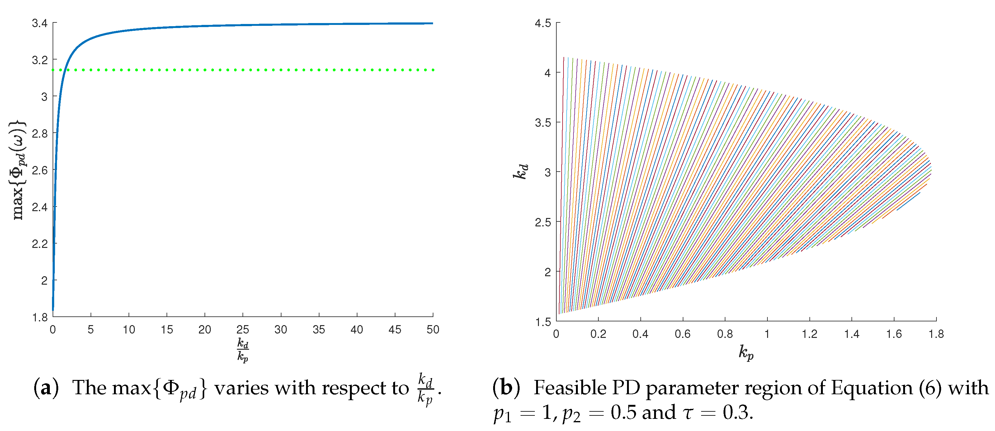
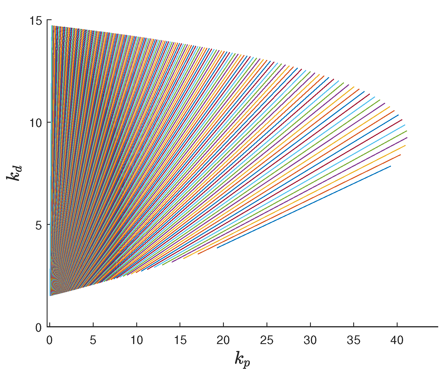
Under PD control, it is easy to obtain the tendency of max $\left\{{\mathsf{\Phi }}_{pd}\left(\omega \right)\right\}$ with respect to $\frac{k_d}{k_p}$ given by Figure 5a. The result in Figure 5a indicates that the maximal phase is larger than $\pi$ for a sufficiently large $\frac{k_d}{k_p}$. It follows that the plant (Equation (45)) may be stabilized by PD and PID control. Next, following Algorithm 1, the feasible PD parameter region is obtained to stabilize the plant (Equation (45)), as depicted in Figure 5b.

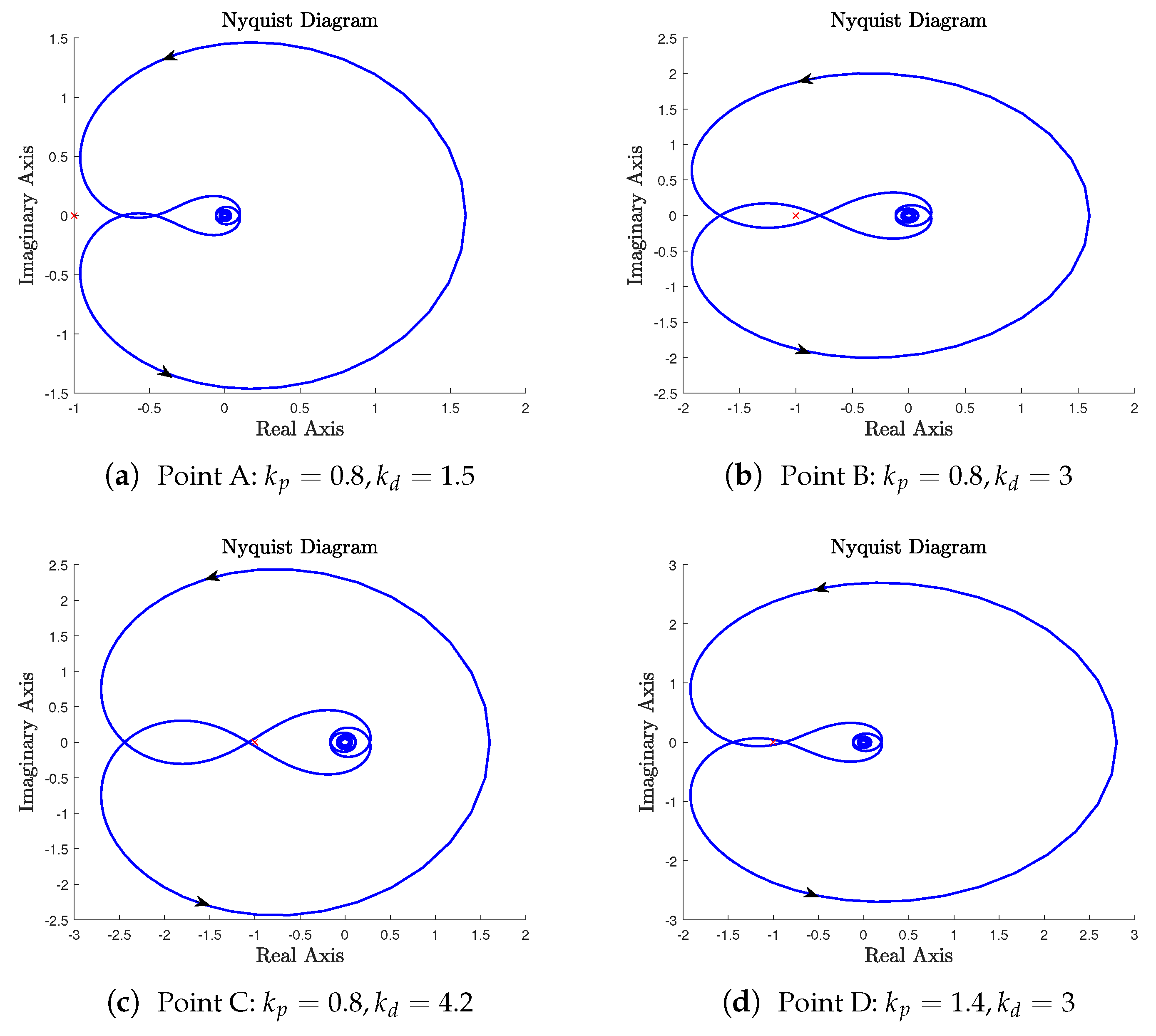
To verify the effectiveness of Algorithm 1, we select $k_p$, $k_d$ arbitrarily in the feasible parameter region in Figure 5b, which are given in

Table 1. $k_p-k_d$ parameters.

	A	B	C	D
$k_p$	0.8	0.8	0.8	1.4
$k_d$	1.5	3	4.2	3

. The corresponding Nyquist curves are given in Figure 6. Figure 6a,c indicate that the Nyquist curves of points A and C encircle the critical point $-1+j0$ zero times, which does not satisfy the Nyquist stability condition. On the contrary, the Nyquist curves of points B and D encircle the critical point $-1+j0$ two times anticlockwise, depicted in Figure 6b,d, which ensures the stability of the closed-loop system (Equation (1)).

Next, the ways in which the time delay may affect the feasible PD parameter region will be discussed. Let us reduce time delay $\tau$ to 0.1. Figure 7 shows that the region will be expanded with respect to the case of $\tau =0.3$ (Figure 5b).

To determine how unstable poles affect the stabilizing parameter region, the stabilization of the plant (Equation (6)) with $p_1=1,p_2=2$ and $\tau =0.1$ under PD control is investigated. Figure 8 indicates that the region will be reduced with respect to the case of $p_2=0.5$ (Figure 7).

It is worth noting that the feasible parameter region depends on both the pole locations of the system and the size of the time delay.

Example 2.

To demonstrate the effectiveness of Algorithm 2 proposed in Section 4.2, a chemical process example proposed by Panda in [34] is to be studied, whose transfer function is

$$P\left(s\right)=\frac{2e^{-0.3s}}{(3s-1)(s-1)}.$$

(46)

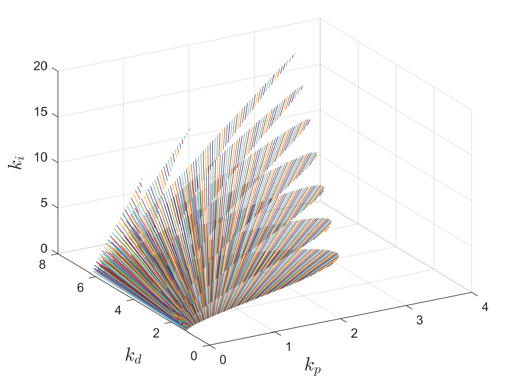
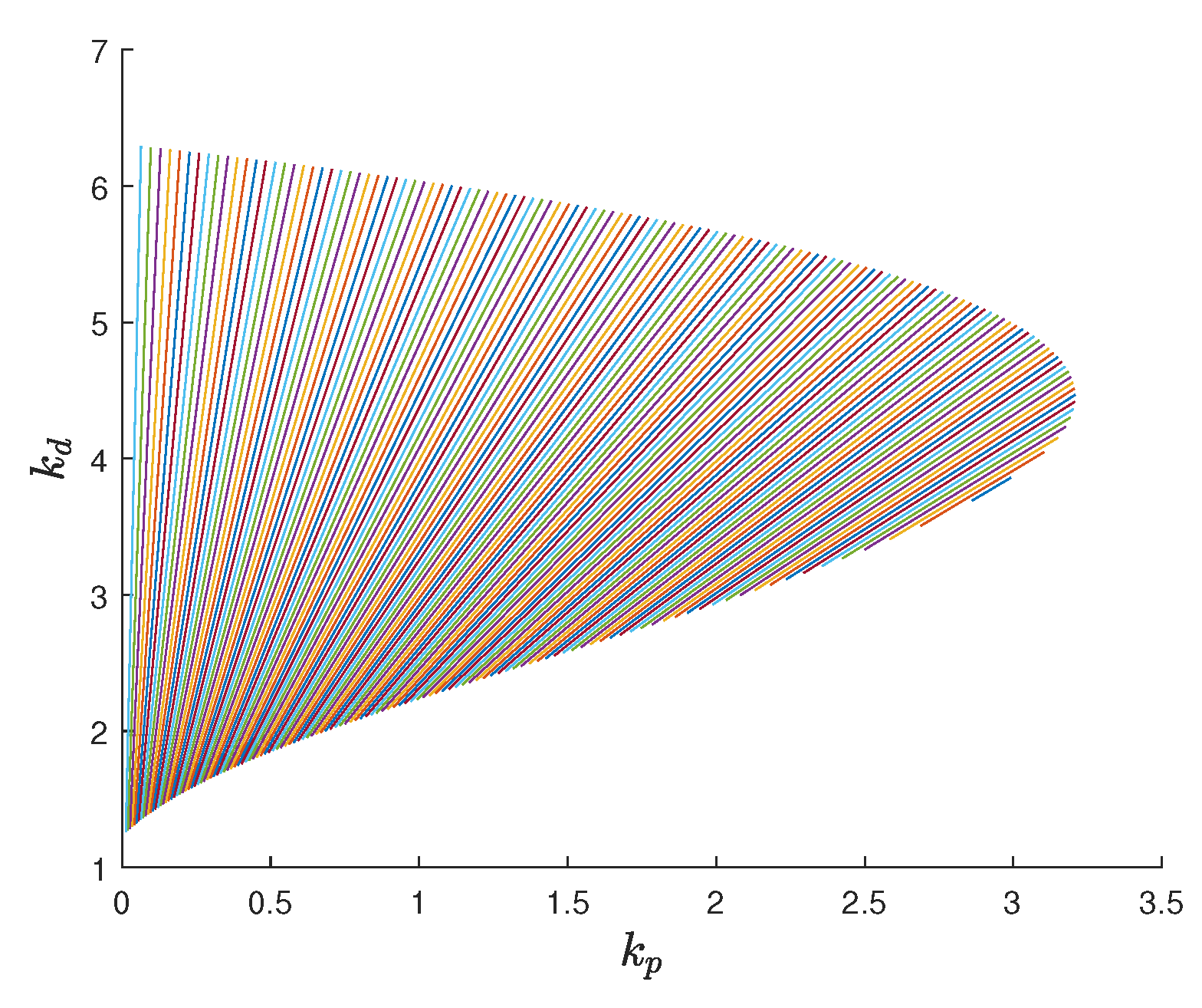
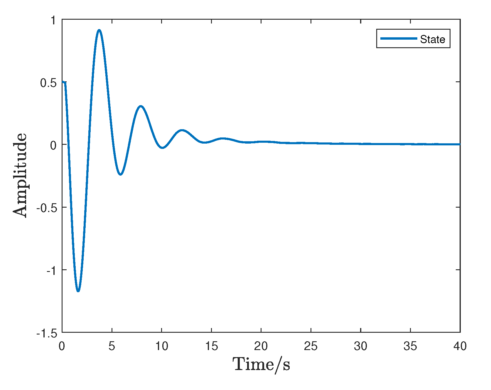
Based on the PID synthesis method proposed in [34], the PID controller is given by $C\left(s\right)=0.881+\frac{0.881}{5.1103s}+3.013s$. On the contrary, by using Algorithm 2, the stabilizing PID parameter region is given by Figure 9. For $\frac{k_i}{k_p}=\frac{1}{5.1103}$, the corresponding parameter region is given by Figure 10. The PID parameters given by [34] are located within our feasible PID parameter region, and the corresponding closed-loop system is asymptotically stable, which is shown in Figure 11. This indicates that we provide the complete feasible parameter region to stabilize the delay systems, while [34] gives the special case with guaranteed performance by placing the closed-loop poles at specific locations.

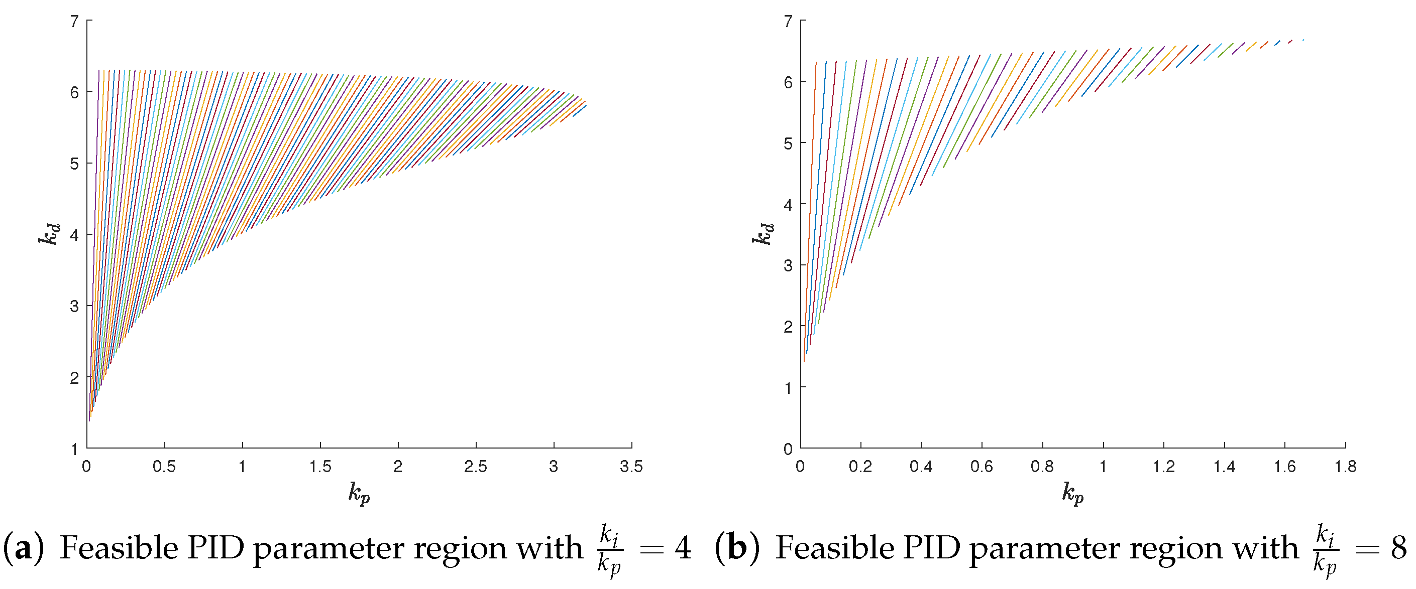
To illustrate how integral control affects the feasible PID parameter region, the corresponding parameter regions are given by Figure 12 with $\frac{k_i}{k_p}=4$ and $\frac{k_i}{k_p}=7$, respectively. It is clear that the feasible parameter region may be reduced if the integral control is enhanced. In the limit, $\frac{k_i}{k_p}=0$ corresponds to the largest feasible parameter region with respect to the projection on the $k_p-k_d$ plane.

The aim of this paper was to find the complete feasible PID control parameter region by using the Nyquist stability criterion. We focused on the stabilization of second-order delay plants with two unstable poles under PID control, but not the optimal PID controller for the specified performance.

From the simulation results, several observations can be made: (i) increasing the delay value may reduce the feasible parameter region; (ii) increasing the poles may reduce the feasible parameter region; (iii) integral control may reduce the feasible parameter region; (iv) a small $\frac{k_d}{k_p}$ corresponds to a smaller phase margin. Even though the best PID gains cannot be ascertained, the above observations may be helpful in obtaining good PID gains. If there exist uncertainties in model parameters, the PID parameters should be chosen with a sufficient margin accordingly.

6. Conclusions

In this paper, the stabilization problem of a second-order delay plant with two unstable real poles is investigated. In contrast to previous works, the methods proposed in this paper are based on the Nyquist stability criterion, which provides an exact and explicit parameter region for delay systems without complex derivation. The stabilization conditions under PD and PID control are proposed, respectively. Moreover, algorithms for computing the feasible PD and PID parameter region are also given. It is safe to conclude that the time delay and integral control may reduce the feasible parameter region through the simulation results.

In this paper, we focus on the second-order delay plants with two real unstable poles. We suggest that this may still be true for second-order delay plants with either one pair of conjugate poles or oscillatory poles. Whether there are novel observations in these cases, a much deeper investigation is required in our future work. In addition, we also note that, to maintain the performance of control systems, the controller and plant model can also be updated online in advanced process control (APC) systems; see, e.g., [35,36]. For details, Fan et al. apply the partial least squares (PLS) method to the MIMO semiconductor processes in the run-to-run (R2R) control practice and address several crucial issues that can realistically occur. Compared with the offline PID tuning approaches, the online algorithms are important to some extent. However, their widespread use depends critically on the real-time capability and reliability of the online algorithms. Hence, from an application point of view, the robustness of our proposed algorithms will be investigated in depth in future work.

References

- Sipahi, R.; Niculescu, S.; Abdallah, C.T.; Michiels, W.; Gu, K. Stability and Stabilization of Systems with Time Delay. IEEE Control Syst. Mag. 2011, 31, 38–65. [Google Scholar]
- Lee, Y.; Lee, J.; Park, S. PID controller tuning for integrating and unstable processes with time delay. Chem. Eng. Sci. 2000, 55, 3481–3493. [Google Scholar] [CrossRef]
- Thowsen, A. An analytic stability test for a class of time-delay systems. IEEE Trans. Autom. Control 1981, 26, 735–736. [Google Scholar] [CrossRef]
- Walton, K.; Marshall, J.E. Direct method for TDS stability analysis. IEEE Proc. Control Theory Appl. 1987, 134, 101–107. [Google Scholar] [CrossRef]
- Sipahi, R.; Olgac, N. Complete stability robustness of third-order LTI multiple time-delay systems. Automatica 2005, 41, 1413–1422. [Google Scholar] [CrossRef]
- Olgac, N.; Sipahi, R. An exact method for the stability analysis of time-delayed linear time-invariant (LTI) systems. IEEE Trans. Autom. Control 2002, 47, 793–797. [Google Scholar] [CrossRef]
- Gu, K.; Niculescu, S.I.; Chen, J. On stability crossing curves for general systems with two delays. J. Math. Anal. Appl. 2005, 311, 231–253. [Google Scholar] [CrossRef] [Green Version]
- Naghnaeian, M.; Gu, K. Stability crossing set for systems with two scalar-delay channels. Automatica 2013, 49, 2098–2106. [Google Scholar] [CrossRef]
- Lanzkron, R.; Higgins, T. D-decomposition analysis of automatic control systems. IRE Trans. Autom. Control 1959, 4, 150–171. [Google Scholar] [CrossRef]
- De Paor, A.M.; O’Malley, M. Controllers of Ziegler-Nichols type for unstable process with time delay. Int. J. Control 1989, 49, 1273–1284. [Google Scholar] [CrossRef]
- Vanavil, B.; Chaitanya, K.K.; Rao, A.S. Improved PID controller design for unstable time delay processes based on direct synthesis method and maximum sensitivity. Int. J. Syst. Sci. 2015, 46, 1349–1366. [Google Scholar] [CrossRef]
- Tan, W.; Marquez, H.J.; Chen, T. IMC design for unstable processes with time delays. J. Process Control 2003, 13, 203–213. [Google Scholar] [CrossRef] [Green Version]
- Seer, Q.H.; Nandong, J. Stabilization and PID tuning algorithms for second-order unstable processes with time-delays. ISA Trans. 2017, 67, 233–245. [Google Scholar] [CrossRef]
- Srivastava, S.; Misra, A.; Thakur, S.K.; Pandit, V.S. An optimal PID controller via LQR for standard second order plus time delay systems. ISA Trans. 2016, 60, 244–253. [Google Scholar] [CrossRef]
- Wang, H.; Liu, J.; Zhang, Y. New results on eigenvalue distribution and controller design for time delay systems. IEEE Trans. Autom. Control 2016, 62, 2886–2901. [Google Scholar] [CrossRef]
- Das, S.; Halder, K.; Gupta, A. Delay handling method in dominant pole placement based PID controller design. IEEE Trans. Ind. Inf. 2019, 16, 980–991. [Google Scholar] [CrossRef]
- Dincel, E.; Söylemez, M.T. Digital PI-PD controller design for arbitrary order systems: Dominant pole placement approach. ISA Trans. 2018, 79, 189–201. [Google Scholar] [CrossRef] [PubMed]
- Zhang, W.; Cui, Y.; Ding, X. An improved analytical tuning rule of a robust PID controller for integrating systems with time delay based on the multiple dominant pole-placement method. Symmetry 2020, 12, 1449. [Google Scholar] [CrossRef]
- Fišer, J.; Zítek, P. PID controller tuning via dominant pole placement in comparison with Ziegler-Nichols tuning. IFAC—PapersOnLine 2019, 52, 43–48. [Google Scholar] [CrossRef]
- Silva, G.J.; Datta, A.; Bhattacharyya, S.P. PID Controllers for Time-Delay Systems, 1st ed.; Springer: Boston, MA, USA, 2007; pp. 135–189. [Google Scholar]
- Yu, X.; Ding, P.; Yang, F.; Zou, C.; Ou, L. Stabilization parametric region of distributed PID controllers for general first-order multi-agent systems with time delay. IEEE/CAA J. Autom. Sin. 2020, 7, 1555–1564. [Google Scholar] [CrossRef]
- Firouzbahrami, M.; Nobakhti, A. Reliable computation of PID gain space for general second-order time-delay systems. Int. J. Control 2017, 90, 2124–2136. [Google Scholar] [CrossRef]
- Hwang, C.; Hwang, J.H. Stabilisation of first-order plus dead-time unstable processes using PID controllers. IEE Proc. Control Theory Appl. 2004, 151, 89–94. [Google Scholar] [CrossRef]
- Zalluhoglu, U.; Kammer, A.S.; Olgac, N. Feedback stabilization of a thermoacoustic device with experiments. In Proceedings of the 2015 American Control Conference, Chicago, IL, USA, 1–3 July 2015. [Google Scholar]
- Lee, S.C.; Wang, Q.G.; Xiang, C. Stabilization of all-pole unstable delay processes by simple controllers. J. Process Control 2010, 20, 235–239. [Google Scholar] [CrossRef]
- Middleton, R.H.; Miller, D.E. On the achievable delay margin using LTI control for unstable plants. IEEE Trans. Autom. Control 2007, 52, 1194–1207. [Google Scholar] [CrossRef] [Green Version]
- Ma, D.; Chen, J. Delay margin of low-order systems achievable by PID controllers. IEEE Trans. Autom. Control 2019, 64, 1958–1973. [Google Scholar] [CrossRef]
- Ma, D.; Chen, J.; Liu, A.; Chen, J.; Niculescu, S.I. Explicit bounds for guaranteed stabilization by PID control of second-order unstable delay systems. Automatica 2019, 100, 407–411. [Google Scholar] [CrossRef]
- Chen, J.; Ma, D.; Xu, Y.; Chen, J. Delay Robustness of PID Control of Second-Order Systems: Pseudo-Concavity, Exact Delay Margin, and Performance Trade-Off. IEEE Trans. Autom. Control 2021. early access. [Google Scholar] [CrossRef]
- Srivastava, S.; Pandit, V.S. A PI/PID controller for time delay systems with desired closed loop time response and guaranteed gain and phase margins. J. Process Control 2016, 37, 70–77. [Google Scholar] [CrossRef]
- Ma, D.; Tian, R.; Zulfiqar, A.; Chen, J.; Chai, T. Bounds on Delay Consensus Margin of Second-Order Multiagent Systems with Robust Position and Velocity Feedback Protocol. IEEE Trans. Autom. Control 2019, 64, 3780–3787. [Google Scholar] [CrossRef]
- Franklin, G.F.; Powell, J.D.; Emami-Naeini, A. Feedback Control of Dynamic Systems, 7th ed.; Pearson: New York, NY, USA, 2015; pp. 333–335. [Google Scholar]
- Xiang, C.; Wang, Q.G.; Lu, X.; Nguyen, L.A.; Lee, T.H. Stabilization of second-order unstable delay processes by simple controllers. J. Process Control 2007, 17, 675–682. [Google Scholar] [CrossRef]
- Panda, R.C. Synthesis of PID controller for unstable and integrating processes. Chem. Eng. Sci. 2009, 64, 2807–2816. [Google Scholar] [CrossRef]
- Fan, S.K.S.; Chang, Y.J. An integrated advanced process control framework using run-to-run control, virtual metrology and fault detection. J. Process Control 2013, 23, 933–942. [Google Scholar] [CrossRef]
- Fan, S.K.S.; Chang, Y.J. Multiple-input multiple-output double exponentially weighted moving average controller using partial least squares. J. Process Control 2010, 20, 734–742. [Google Scholar] [CrossRef]
Figure 1.
Unity feedback system.
Figure 2.
Nyquist curve with for stabilization of the plant (Equation (6)).
Figure 3.
Nyquist curve with for stabilization of the plant (Equation (26)).
Figure 4.
Nyquist curve with for stabilization of the plant (Equation (31)).
Figure 5.
Stabilization under PD control. The first figure indicates that the maximal phase is larger than for a sufficiently large . The second figure show the set of stabilizing PD parameter.
Figure 6.
Nyquist curves of the plant (Equation (45)) for different PD parameters.
Figure 7.
Feasible PD parameter region with and .
Figure 8.
Figure 9.
Feasible PID parameter region of the plant (Equation (46)).
Figure 10.
Feasible PID parameter region with .
Figure 11.
System state under PID control with .
Figure 12.
Feasible PID parameter region. The above two figures show the feasible PID parameter region with and .