
Advanced Design and Optimal Sizing of Hydrostatic Transmission Systems


Maha Fluid Power Research Center, Purdue University, West Lafayette, IN 47907, USA
*
Author to whom correspondence should be addressed.
Actuators 2021, 10(9), 243; https://0-doi-org.brum.beds.ac.uk/10.3390/act10090243
Submission received: 12 August 2021
/
Revised: 13 September 2021
/
Accepted: 17 September 2021
/
Published: 21 September 2021
(This article belongs to the Special Issue Fluid Power Actuation Systems)
Abstract
:This paper presents a novel method for designing and sizing high-efficient hydrostatic transmissions (HTs) for heavy duty propulsion applications such as agricultural and construction machinery. The proposed method consists in providing cost effective HT architectures that maximizes efficiency at the most frequent operating conditions of the transmission, as opposed to the traditional HT design methods based on the most demanding requirements of the system. The sizing method is based on a genetic optimization algorithm for calculating the optimal displacement of the main units of the HT to maximizes the efficiency in the most frequent operating conditions of the vehicle. A simulation model for HTs is built in MATLAB/Simulink® environment to test three different circuit alternatives for basic HTs. Considering a particular 250 kW heavy-duty application for which drive cycle data were available, this study shows great improvement in energy efficiency (14%) and power saving (20.1%) at frequent operating conditions while still achieving the corner power condition.
1. Introduction
Hydrostatic transmissions (HT) are the most common technology to control propulsion in off-road vehicles such as gardening machines, tractors, harvesters and many more. Continuously variable transmissions (CVT) are a form of hydrostatic transmission that allow power transmission from the engine to the wheels with a continuously variable ratio, thus allowing optimal propulsion relations, in terms of wheel torque vs. vehicle speed, almost independent of the engine torque characteristic [1] Compared to other hydraulic control architectures, such as metering control systems, HTs have also the advantage of not introducing dissipative fluid throttling. For this reason, HTs are among the most efficient fluid power transmission systems. There are numbers of different architectures of HTs. The basic layout of the hydraulic system can be either open-circuit or closed-circuit. Closed circuit HTs are more common in heavy duty applications, because of the less stringent requirement on the oil-reservoir size, and their ability to operate in four quadrants, in terms of vehicle velocity and wheel torque [2,3].
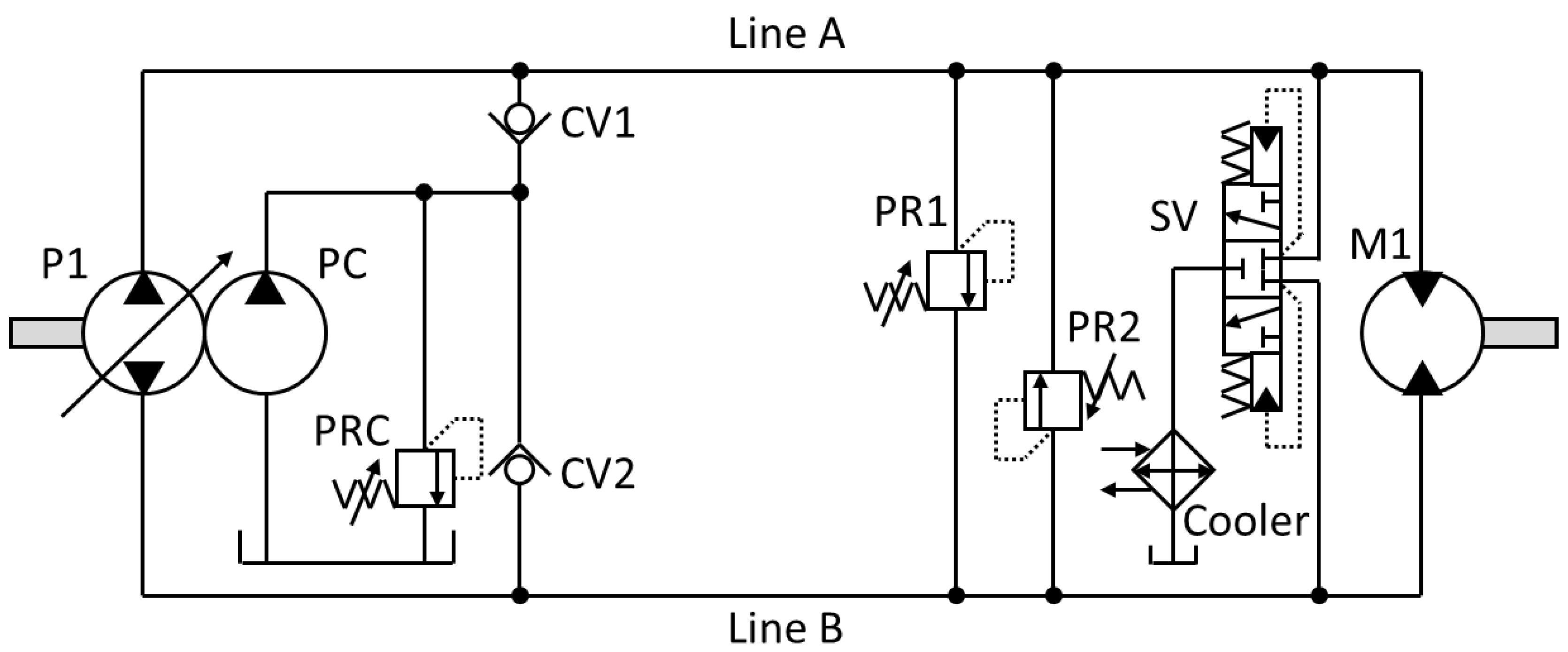
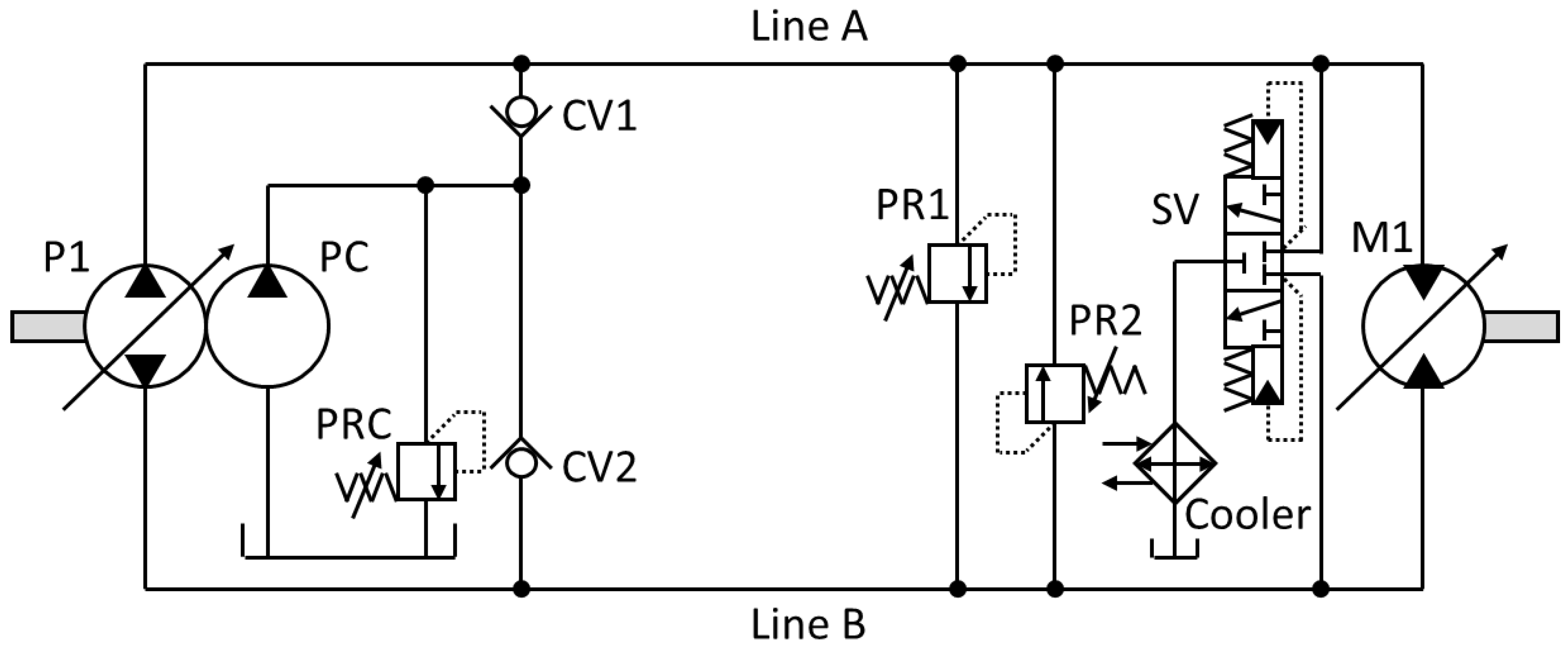
The basic schematic of a closed-circuit HT is shown in Figure 1. Typically, one variable displacement hydraulic unit (pump, or primary unit) is mechanically connected to the prime mover (i.e., the combustion engine) and exchanges hydraulic energy with one or more hydraulic units (motor or secondary unit) connected to the wheel axle(s). The secondary unit can be either a fixed or variable displacement. As shown in Figure 1, usually the HT includes a shuttle valve (SV) for oil cooling (Cooler), a cross port pressure relief valve (PR1&2) for protection from pressure overload and a charge circuit (PC, CV1, CV2, PRC) for oil replenishment. Different variants to the basic architecture of Figure 1 exist, as pertains to the charge circuit, the connections of multiple motors, in either series or parallel configurations, and on the flushing circuit. Significant examples can be found in [2,3,4,5].
The main challenge in designing an HT is to determine the type (either fixed or variable displacement) of the hydraulic units and finding their size in terms of displacement in (cc/rev). As will be discussed next, this sizing process is typically based on static considerations about the engine power and the requirements of the vehicle propulsion system.
Design of Reference HT System
There are not many sources in the literature that guide a designer towards the sizing of an HT for a given vehicle. The most complete design procedure known to the authors is the one detailed by Zarotti [3], which is also summarized in [4]. According to the above source, the most convenient architecture for an HT to achieve a CVT can be based on either a fixed displacement motor or a variable displacement motor, based on a parameter referred to as Torque Conversion Factor (TCF). The TCF is the ratio between the corner power of the transmission and the maximum power of the engine. The corner power of the transmission can be calculated from the maximum tractive effort of the vehicle and its maximum travel velocity, which are both application-specific. The corner power of the HT can be higher than the engine power, particularly for applications where the propulsion is the most power demanding hydraulic consumer. When the difference between the HT corner power and the engine power is high (high TCF), variable displacement motors are more advantageous. Instead, for low values of TCF it is convenient to use fixed displacement motors. This rule is supported by a lot of practical evidence, and it is aimed at extending the CVT function at the maximum power level of the engine for a wide range of vehicle velocities. In [6] Paoluzzi and Zarotti further refine this sizing procedure, providing further considerations about the vehicle class, and providing additional criteria for selecting the HT architecture type, including the use of multiple hydraulic motors.
Although some basic considerations about energy transmission efficiency are stated in [6], the HT energy efficiency during the typical mission cycles of the vehicle is an aspect often overlooked during the sizing process. This is true even if the propulsion is often a primary function for the vehicle, from the energy demand point of view. Outside the best operating points, the overall efficiency of an HT can be significantly low (even less than 40%), and it can be hardly higher than 80% in the best operating conditions. Even if the system does not introduce fluid throttling between the primary and secondary units, significant power losses are still present due to the low performance of the positive displacement machines at partial displacement [7]. Other factors such as both the charge and the flushing circuits also affect the HT’s efficiency.
Several past studies addressed the modeling and the analysis of the HT with particular focus on the transmission efficiency. One of the most recent works is the analysis performed by Sing et al. [8], where the efficiency of a typical closed-circuit HT is evaluated through numerical simulation. This work confirmed the finding, also well discussed by Manring in [9], that the steady-state efficiency of the HT is mostly determined by the overall efficiency of the primary and secondary units. An exhaustive analysis of the energy losses occurring in positive displacement machines suitable for HTs, depending on the operating conditions, is detailed in [7]. The overall efficiency of the transmission is also highly affected by the efficiency of the prime mover. An exhaustive analysis of the HT transmission efficiency is also performed by Costa and Sepehri [5]. These works, however, focus on given units and do not provide a specific procedure for sizing the transmission to maximize the efficiency during operation. Another source of loss in HT efficiency is the low-pressure charging circuit. Keller et al. conducted a detailed study on the sizing and energy impact of the low-pressure system in closed-circuit hydraulic transmission [10].
More significant is the effort made by researchers in the fluid power community towards the proposal of modifications of the basic HT schematic aimed at improving the system efficiency. After the first pioneer work published by the John Deere company [11,12] several HT architectures based on the so-called hydromechanical power-split architecture were proposed. A hydromechanical power split uses a planetary gear train to merge an HT with a mechanical drive in a single transmission. This type of design adapted the advantage of the CVT capability of hydraulic transmission while keeping the high efficiency nature of a purely mechanical transmission, but it comes with a much higher implementation complexity and cost, which limits its application to certain high productivity vehicles such as agricultural tractors. Examples are the systems discussed in [13,14,15]. Even higher energy transmission efficiencies can be achieved by hydraulic hybrids (see classifications provided in [16]), where architectures claimed to achieve transmission efficiencies comparable to electric hybrids, therefore being suitable for on-road applications [17,18]. Kumar and Ivantysynova proposed a power management strategy base on instantaneous optimization [19,20]. His result shows great reduction in fuel consumption: 28% on the highway and 13% in city driving. Heikkilä et al. used dynamic programming to optimize fuel efficiency on a wheel loader, also showing great energy savings [21]. Sprengel and Ivantysynova used neural network-based power management on a hydraulic hybrid transmission. His controller was tested on a hardware-in-the-loop test rig and shows up to 25.8% fuel saving [22].
Although the works cited in the last paragraph do not apply to basic HT architectures like the one of Figure 1 that dominates the off-road vehicle applications, these past contributions, particularly [15,17,18,20,23] are still relevant to this paper. This is because these past works outline methodologies for optimizing the design of the hydraulic control system with respect to energy efficiency over specific utilization cycles.
The basic HT layout, consisting of one primary and one secondary unit, has indeed very limited regulation flexibility for addressing system efficiency. This was already commented by Paoluzzi and Zarotti in the work previously cited [6], and an aspect they further addressed in their more recent work [24] where they discussed simple modification to the basic architecture by acting on the number of primary and secondary units. This latter work presented three different improvement designs to expand the working range of HTs and to further expand the sizing method first presented in [6]. One improvement they presented is based on a mechanical gearbox with a dual motor design, which increases the working range of the HT with a little complexity added. The results show great flexibility for adaptation to different applications as well as potential efficiency gain as additional benefit. However, the introduction of an additional gearbox can be prohibitive from the point of view of the cost in a commercial application.
From the above discussion about the state of the art of the design techniques for basic HTs, it appears evident how it is still of interest to provide viable (i.e., cost effective) modifications to the basic HT schematic of Figure 1, along with proper sizing methods that can bring improved transmission efficiency. The past studies clarify that an additional control degree of freedom must be introduced to the HT to allow for better working conditions of the hydraulic units, to decrease the power loss. The open question is where the most convenient place is to introduce such freedom. By inspection of the typical efficiency maps of the primary and secondary units, which will be discussed in a later section, the unit displacement and the system pressure are the most important parameters effecting the system efficiency. In this work, three HT design improvements that allows such type of modification will be proposed. In particular, a split pump design and a dual displacement motor will be considered as alternative HT configurations to the baseline system of Figure 1.
The purpose of this work is to provide a design method for HTs to achieve maximum energy efficiency considering real working conditions, while still meeting the vehicle requirements in terms of extreme working conditions. The architecture selected as reference for this work is the one of Figure 1, with design requirements typical of harvesters used in agriculture.
The paper describes how the above objective is reached with the following structure. Section 2 discusses how the HT efficiency can be defined with respect to the vehicle speed and loading conditions. Then, Section 3 introduces the proposed HT designs in detail and explains how these new designs affects the system functionality and its efficiency. The same section lays out the system control strategy of such systems. Section 4 describes the optimization method based on a genetic algorithm used to size the HT to achieve maximum system efficiency. Section 5 presents the modeling of the proposed HT systems. Finally, Section 6 presents a case study of a representative off-road application (i.e., a harvester), where a particular drive cycle is considered to estimate the energy consumption advantages of the proposed solution.
2. HT System Efficiency
Among the different sources of inefficiency in an HT, such as volumetric and hydromechanical losses of the primary and secondary units, unit control system loss, cooling loss, losses in the charge pump and flushing circuit, this study focuses on the volumetric and hydromechanical losses as they are the most dominant loss in a closed-circuit HT [9]. It is worth mentioning that modifications to the low-pressure charging system, which is associated to the control system loss and cooling loss, also has potential for improvements, as discussed in [25]. However, this is not the focus of this work, which assumes no modifications made on the architecture of the charge system
Losses in the hydraulic primary or secondary unit are the volumetric loss and the torque loss [7], which are often expressed in terms of volumetric efficiency, representative of the flow loss , and hydromechanical efficiency, representative of the torque loss . These losses can be expressed as a function of the working conditions:
where is rotational speed for the pump or motor, is pump or motor displacement, is the pressure difference across the delivery and suction port of the units and is the unit maximum displacement.
There are three approaches generally used to accurately model these unit losses. First, there are analytical loss models based on empirical parameters. Examples of these are in [6,7,9]. This type of model is based on the tuning of some key parameters in physical formulas from experiment data. The advantage of these empirical models is that they are fast and based on physical equations. However, it is difficult to obtain experimental data to accurately tune these constants for any existing unit. Second, there are tribological-based models, which evaluate the losses by solving the lubricating gap interfaces present in a positive displacement machine. Examples are the model developed by Pelosi and Ivantysynova [26] and Chen et al. [27]. Using such models is computationally very expensive. These models are usually suitable for the analysis and the design of single interfaces (such as the piston–cylinder interface or the slipper–swash plate interface of a piston pump), but they are not readily available for omni-comprehensive simulation at a system level. Third, it is possible to use look-up tables that reflect experimental data. This method is purely based on experimental data and does not require modeling equations. Among these options, for this work the unit loss look-up tables approach was used.
By having the unit losses available in terms of look-up tables, a good base for the system efficiency is found. However, it is also necessary to link the unit loss model with the whole range of working conditions for the HT, in terms of vehicle speed and wheel resistance. Following the method proposed in Manring [9], the overall HT system performance can be derived using the following equations for the pump rotational speed (3); the motor speed, which can obtained from the track rolling radius and the motor gear ratio (4); the corresponding pump instantaneous displacement (5); and finally the system differential pressure calculated (6). is the gear ratio of the units to the engine and track, is the vehicle speed, is the rolling radius of the track, is the volumetric/hydromechanical efficiency for pump/motors and is the machine load force.
With the above equations related to the HT performance, the whole working range of the vehicle is mapped directly to the pump and motor working conditions uniquely. Then, the pump and motor volumetric and hydromechanical efficiency is calculated through Equations (7)–(10). Finally, the whole HT system efficiency is simply the product of all pump and motor volumetric and hydromechanical efficiency as shown in Equation (11).
3. Reference and Proposed HT Systems
This section presents the HT solutions considered in this study, referred to as Solution A, B, and C. Solution A gives the best loss reduction and efficiency gain but with most additional components. Solution B and C are a compromise between additional components and energy saving. These solutions will be considered with specific reference to applications such as heavy-duty harvesters, which operates at relatively constant vehicle speed and drag load.
3.1. Reference HT System
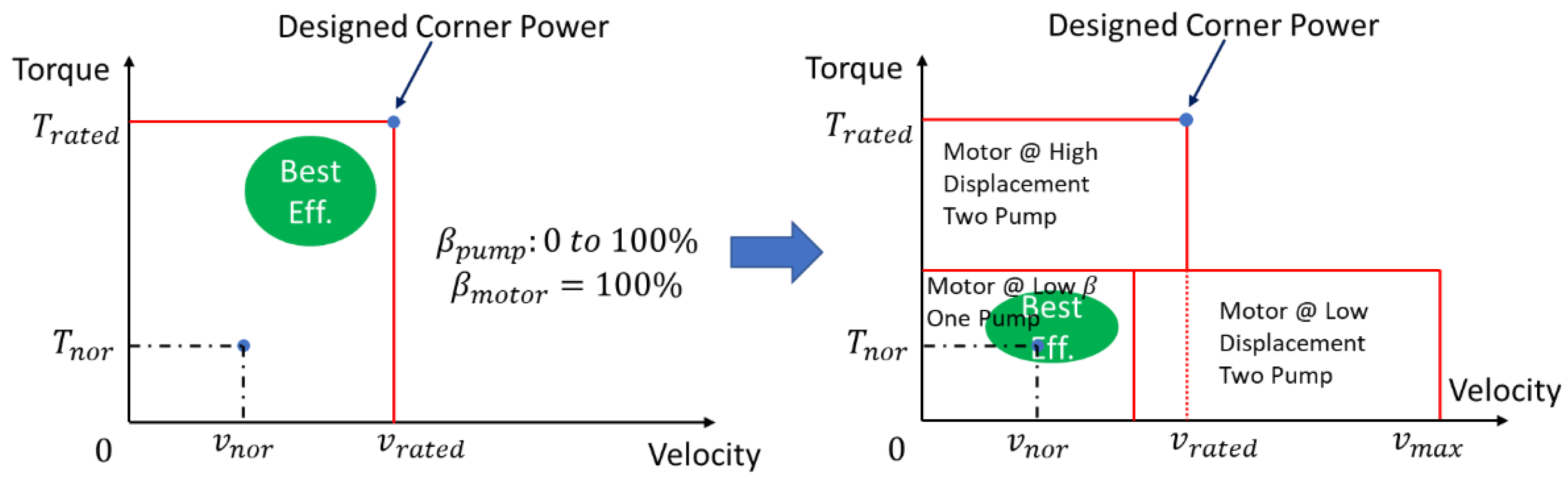
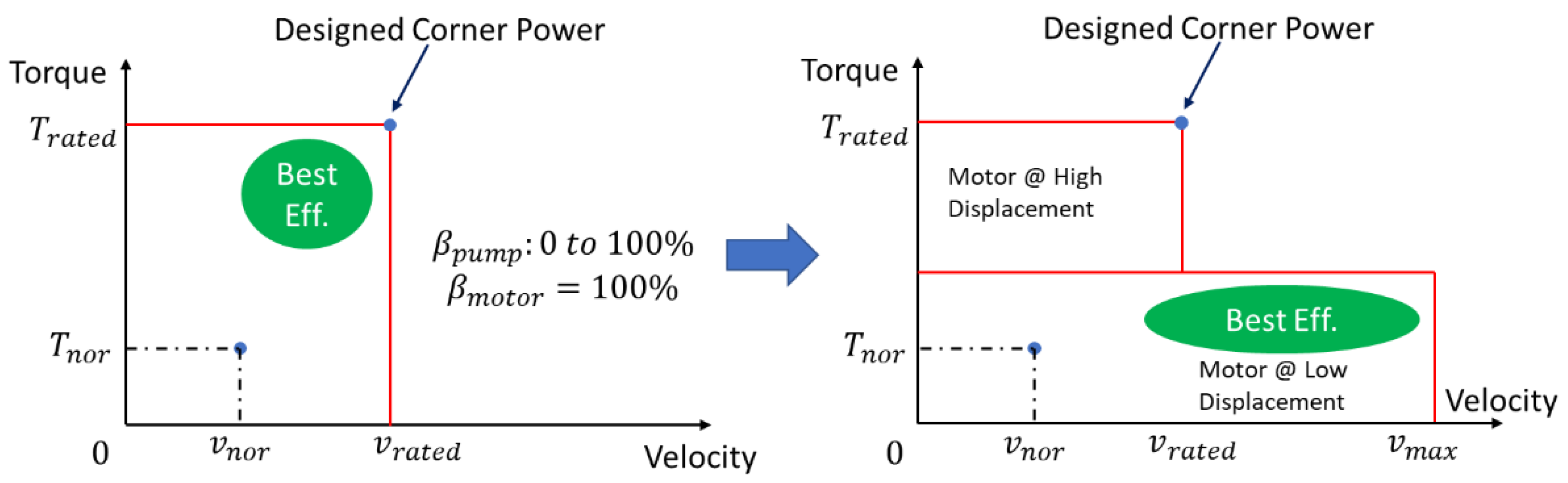
For the type of vehicle considered in this study, the typical HT follows a schematic such as the one of Figure 1, which includes one variable displacement hydraulic pump and one fixed displacement motor. This schematic will be considered as baseline reference. Figure 2 shows the operation condition for the reference HT system. The upper-right blue dot is the designed corner power condition with respect to machine rated maximum speed and rated maximum load torque .
The corner power condition corresponds to the most demanding working condition, but it is normally far from the most frequent operating condition of the machine , where the machine spends most of its time. By inspecting the hydraulic system design of different harvesters, it is common that the most frequent operating vehicle speed is at around 50% of the rated maximum vehicle speed and the vehicle load torque is at around 25% of the rated maximum vehicle load. From Manring [9], it appears that the best efficiency range for HT system is at medium to high load torque and vehicle speed as shown in the above figure. As a result, the most frequent operating condition does not overlap with the best efficiency range, thereby bringing significant power loss.
The following solutions are proposed to add system control freedom, with the goal of reshaping the HT operating map to align the best efficiency range with the most frequent operating condition. It must be observed that in case a given HT already operates near the best efficiency range, this method will not provide much improvement like the case presented in this paper.
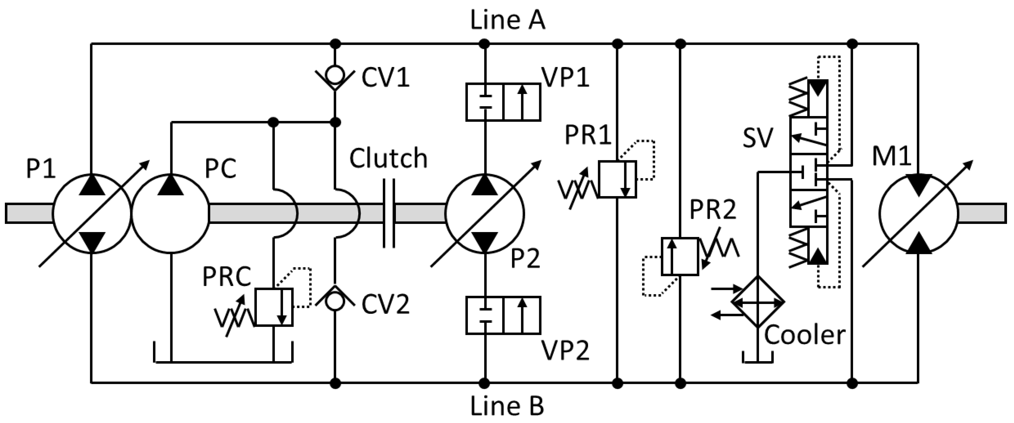
3.2. Solution A
Hydraulic pumps and motors achieve optimal values for the overall energy efficiency at medium/high differential pressure and high displacement. For a given operating condition of the HT (i.e., output torque and speed), the unit displacement and working pressure can manipulated by adding a degree of freedom, such as a variable displacement motor or with additional pumps. In Solution A, shown in Figure 3, the pump is replaced by two smaller variable displacement pumps (P1 and P2). P1 is designed to operate during the most frequent operating condition, while P2 is used to provide additional flow to reach the rated maximum vehicle speed. In addition, the hydraulic motor (M1) uses a two-position displacement technology. The low displacement setting for M1 is used for most frequent operating condition, raising the overall system efficiency through higher system working pressure difference. There is a tradeoff between motor displacement values and the achievable differential pressure that will be found by the optimization process described in this work. The high displacement setting for M1 is only used for high torque mode when the rated maximum vehicle output torque is required. Two isolation valves (VP1 and VP2) and one clutch between pumps are used to isolate P2 during the most frequent operating condition. By doing this, P2 will not introduce any parasitic losses to the system when not active. If the machine needs to reach high power conditions (near corner power), P2 will engage, and the motor will set its displacement to high. All other components (charge pump PC; check valves CV1 and CV2; relief valves PRC, PR1 and PR2; shuttle valve SV and cooler) have the same function as the reference HT system. A more detailed explanation on the control strategy for this solution is provided in the following section.
With the assumption that the total displacement of P1 and P2 in Solution A is the same as the displacement of P1 in the reference machine and the motor is the same size as the reference machine as well, the effect on the HT operating range given by Solution A with respect to the reference system of Figure 1 is shown in Figure 4. The left plot of Figure 4 shows the working range of the reference HT system with the designed corner power (rated maximum vehicle speed and load). By adding P2 and a two-position motor, Solution A enlarges the range of operating velocities and will also be able to achieve the corner power condition. The enlarged velocity range is because the motor could lower its displacement, so the machine potentially can travel at higher speed than the rated speed as shown in Figure 4 right. Most importantly, for the most frequent operating condition, the transmission can operate at its best efficiency, as shown in Figure 4 on the right.
3.3. Solution B
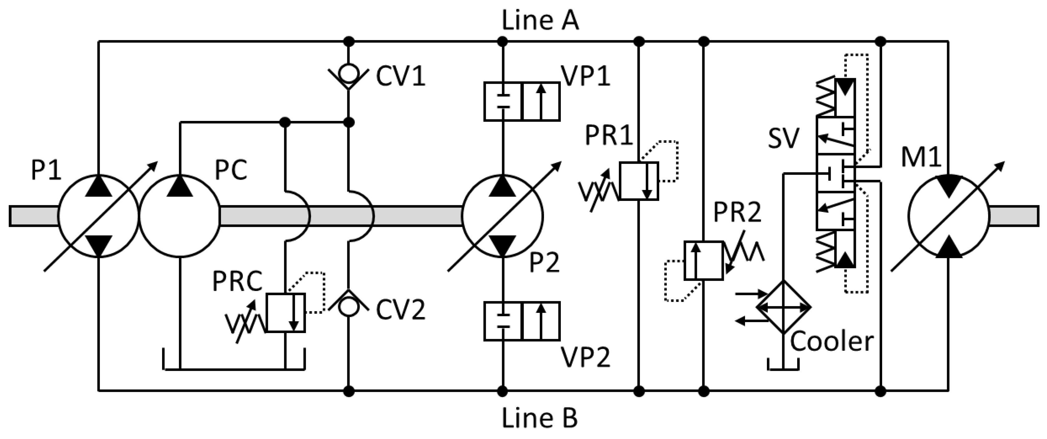
Similar to Solution A, Solution B also uses two pumps and one two-position motor. The difference is the absence of the engaging clutch mechanism for P2, as shown in Figure 5. Such mechanism might affect cost and reliability and therefore might not be suitable for certain applications. Without the clutching system, with Solution B the two pumps are always connected to the prime mover. Therefore, P2 introduces parasitic losses to the system also when it is not actively used. For the remaining components as well as the operating control logic and range, Solution B is basically the same as Solution A.
3.4. Solution C
Solution C is a one pump–one motor architecture, like the baseline system. However, Solution C uses a dual displacement motor instead of a fixed displacement one (Figure 6). As pointed out in [3,6], this transmission type is more suitable for high TCF values, allowing for better engine utilization in terms of power. The solution has a limited cost increase, compared to the previous Solution A and B.
In this solution, in the absence of the additional degree of freedom at the pump side, like in the Solution A and B, the pump P1 will need to run at low displacement in most of the working conditions, with a detrimental effect on the overall HT efficiency. Figure 7 shows the operation range change for Solution C.
3.5. HT System Control
The HT schemes presented in the last section show basic HT layouts that use a variable displacement pump with either a fixed displacement motor or a two-position motor. The two-position motor can be considered as a fixed displacement unit, when it operates at a particular setting. Therefore, the strategy for controlling the unit displacement for all presented solutions can be straightforward. The vehicle HT system is controlled using speed control logic. The vehicle speed can be related to the pump displacement linearly (assuming a negligible effect of the volumetric losses in the units, which can be compensated by a proper controller as explained in the following). When the HT is at a standstill, the pump is at minimum displacement (ideally zero). When the driver requests higher speed, the pump displacement increases to certain level to achieve the requested speed. This procedure can be considered for the reference system of Figure 1.
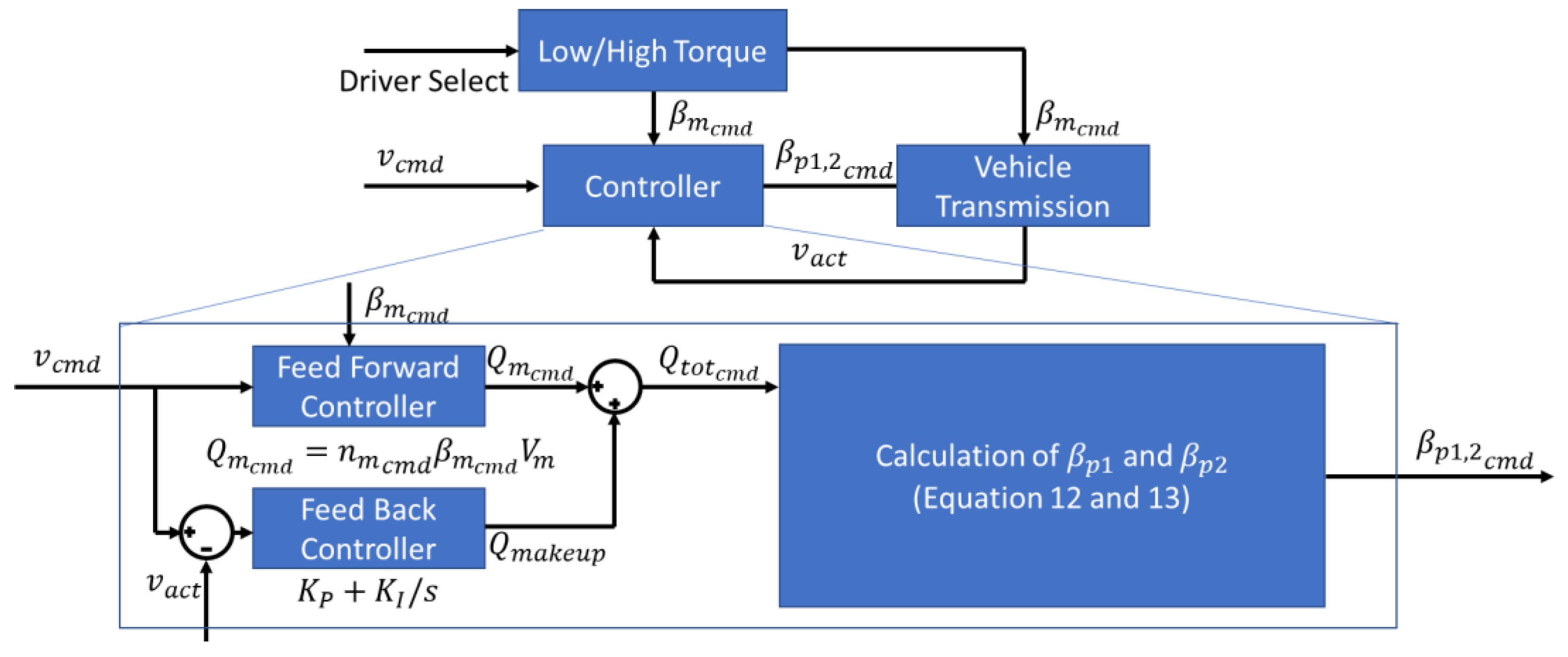
Solution A and B use the same control logic, as the only different between them is the presence of the clutch. Due to the dual pump architecture and the two-position motor, the control logic would implement proper modification compared to the reference HT system. Figure 8 shows the control block diagram for the proposed Solution A and B.
First, the operator will choose if the machine needs to be in high or low torque mode. This alone will determine the motor position : either low displacement for the most frequent operating mode or maximum displacement for high torque mode. Then, the controller takes the motor position information and the requested speed to calculate the two pump displacements . A feed-forward and a feedback controller are used to precisely control the vehicle speed. The feed-forward controller calculates the theoretical flow rate needed from the pump to achieve the requested vehicle speed. The feedback controller is a proportional–integral (PI) controller to monitor and correct any speed error by providing makeup flow for volumetric loss of the pump and motors. Both flows will be added together as the total flow required to calculate the displacement of P1 and P2. If the total flow required is lower than the maximum flow of pump P1 , then the P1 displacement will be calculated and P2 will remain at zero displacement and become isolated from the system (close VP1, VP2 and open the clutch for Solution A) to reduce the loss as in Equations (12) and (13) condition. If the total flow required is higher than maximum flow of P1, then P1 is held at maximum displacement and P2 will engage (open VP1, VP2 and close the clutch for Solution A) to provide flow in addition to the flow P1 already provides as in Equations (12) and (13) condition.
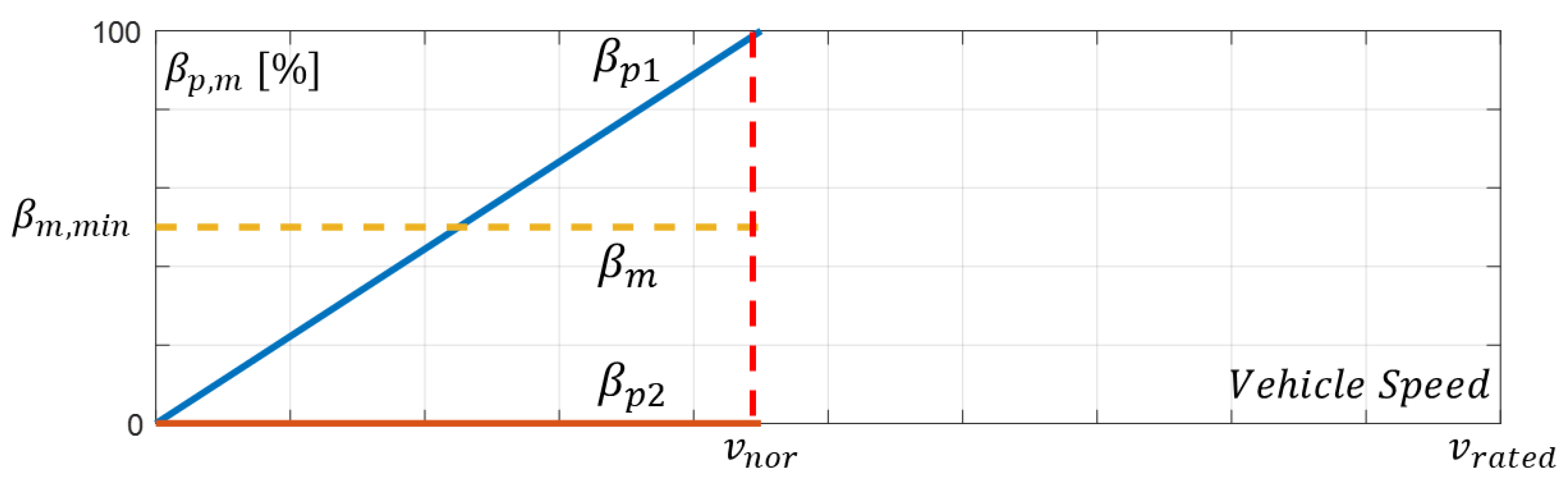
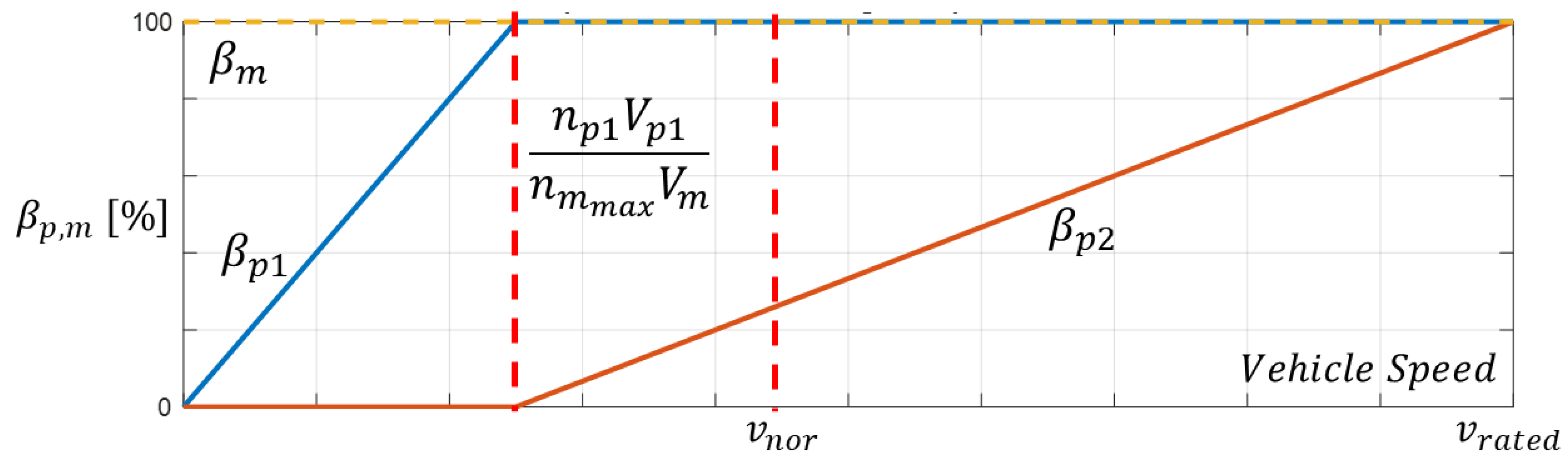
For the most frequent operating conditions, it is convenient to have P1 providing flow near its maximum displacement, while P2 is isolated by means of the clutch and the on/off valves. In this condition, the hydraulic motor operates at the low displacement setting. Figure 9 shows the displacement change vs. vehicle speed for near the most frequent operating condition mode. At standstill, P1 is at zero displacement. When a higher speed is requested, only P1 increases the displacement. When the P1 reaches its maximum displacement, the vehicle is slightly faster than the most frequent operating condition vehicle speed (50% vehicle speed). Vehicle deceleration occurs with a similar, but reversed, procedure.
In the high torque mode, both pumps are engaged, and the motor is at its maximum displacement setting. Figure 10 shows the displacement change vs. vehicle speed for the high torque mode. At standstill, both pumps are at zero displacement. When higher vehicle speeds are requested, P1 will first increase displacement while P2 stays at zero displacement. When vehicle speed reaches , P1 reaches its maximum displacement. Then, P2 starts to increase the displacement to provide more flow to reach a higher vehicle speed. Finally, when P1 and P2 both reach their maximum displacement, the vehicle reaches the maximum allowable speed. The pumps and motor size from the optimization should ensure that this maximum speed is always higher than the vehicle rated maximum speed to satisfy the vehicle performance requirement. An event of vehicle deceleration would occur with a similar, but reversed, procedure.
Solution C also has two modes of operation. However, because it is still a one variable pump plus one fixed motor configuration, the control logic is the same to the reference HT system within each mode.
4. Optimization
This section describes the optimization algorithm used to size the alternative HTs introduced in the previous section, with the goal of achieving the maximum overall energy efficiency. The system to be optimized is non-linear and many of its variables are discontinuous, which means that the optimization algorithm has to be suitable to solve this kind of problem. A few examples of such algorithms are the genetic algorithm [28], machine-learning [29], the Nelder–Mead method [30], etc. The genetic algorithm is the choice in this work because it is suitable for these features and provides a global minimum. As a drawback, the genetic algorithm can be computationally expensive for complex systems. This complexity includes the number of design variables, the target system working conditions, and the objective functions.
Some actions were taken to reduce the complexity of the optimization problem to promote a faster optimization. First, a single point optimization was considered instead of an entire vehicle drive cycle. This operating point corresponds to the most frequent operating condition that can be detected in the drive cycles. This simplification is appropriate for vehicles such as harvesters that are designed to maintain an approximately constant vehicle speed and load. Second, because of the above simplification, the solution of the HT used in the optimization does not need to consider all the transient aspects of the hydraulic system, such as an instantaneous pressure dynamic, vehicle dynamic or hydraulic valve dynamic behavior. By conducting these simplifications, the computational requirement of optimization allows for fast results.
4.1. Design Variables and Operators
For all the proposed HTs, the design variables are chosen as listed in Table 1. As pertains to the pump and motor population, a discrete set of values coming from an existing commercial product line is considered. From these selections, the available pump and motor sizes are represented as and . The range of the motor in the most frequent operating displacement is chosen to be between and .
For the genetic algorithm set up, this work follows the method introduced in [28]. Each of the design variables need to be converted into a piece of binary code with a certain number of bits. For discontinuous design variables, the binary code needs to have enough bits to include all possible designs. For example, a 4-bit binary code could represent different combinations, which is enough for 16 different pump or motor sizes. For continues design variables, the variable range and bits will determine the resolution for the optimization of this variable. Taking the motor displacement as an example, the variable range is . The desired resolution is smaller than , which means the variable range needs to be divided into at least pieces. If this number is above 516 and below 1024, then a 10-bit section of binary code could be assigned for it, which could represent pieces. The final resolution is .
For the population size, it is a normal practice to start with four times the total bits sum. The cross over rate is chosen to be 50% and the mutation rate is 0.5% to ensure global optimum result. The termination criterion is when fifty consecutive generations end up with same best fitness. The maximum number of generations is 500.
4.2. Objective Function Definition
The objective function is key for any genetic algorithm. In this work, the objective is to maximize the overall system efficiency which is defined using Equation (11). As discussed earlier this transmission system efficiency is heavily dependent on the displacement settings of both the hydraulic pump and motor. Equations (3)–(6) are used to transfer the design variable and vehicle working condition into the unit working condition. Then, to calculate the overall system efficiency, the empirically derived unit loss model is used, which was introduced in Section 2, and it will be further discussed later in Section 5.
4.3. Constraints
Constraints are applied to ensure feasibility of the solutions considered by the algorithm. First, the system operation pressure should be kept below a maximum value for safe operation of the system (14). Second, the motor shaft speed must stay within the rated maximum speed (15). Third, during most frequent operating condition, P1 alone should provide all the flow (16). As the last constraint, the system must reach the corner power condition (17), (18). These constraints are analytically expressed as follows:
5. Simulation Model
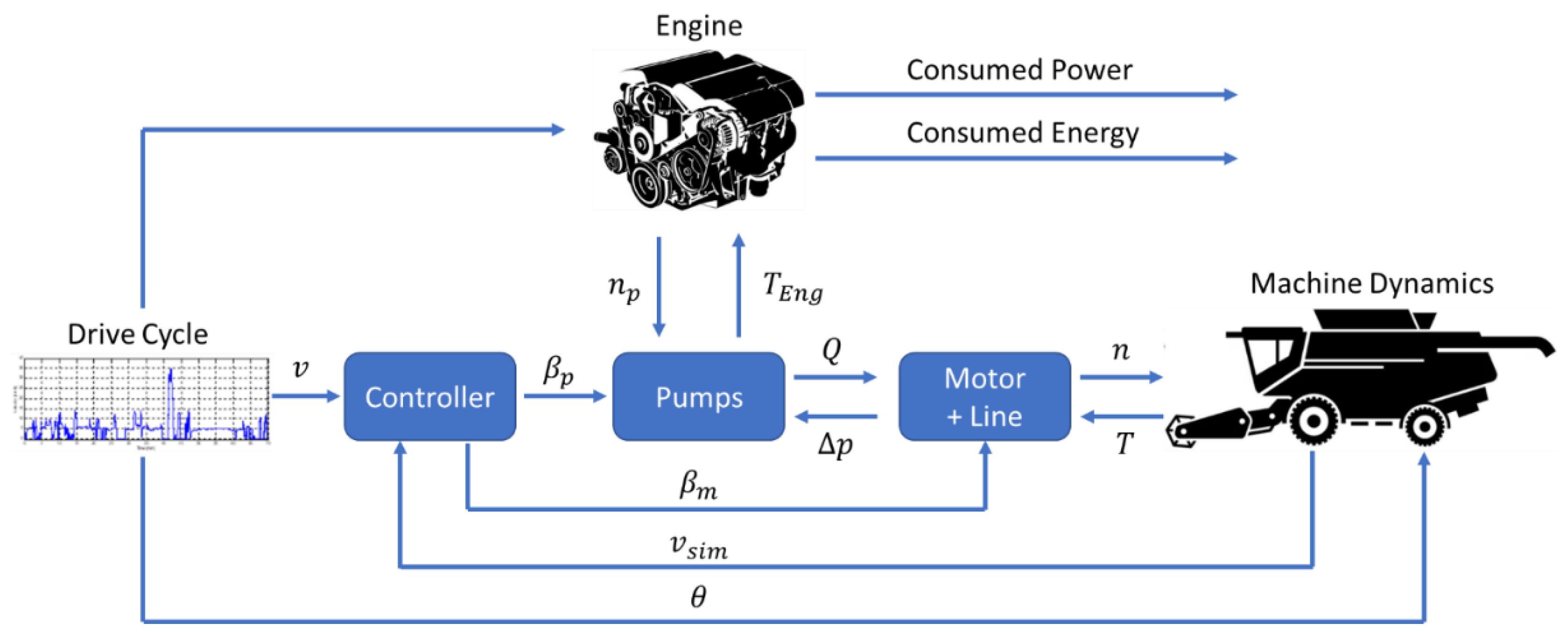
Although the optimization algorithm considered that the pump and motors are working under stationary operating condition, near constant speed and load, a dynamic simulation model was developed within this research for more realistic predictions. Even if the drive cycle of an agricultural machine such as a harvester operates mostly near a fixed point, during a real drive cycle the HT may also encounter points different from the one assumed in the optimization. For this reason, this paper also considers a realistic simulation of a specific harvester operating on a given drive cycle as opposed to the constant operating point used during the optimization process. Therefore, the optimized sizing for each HT configuration is evaluated by simulating a real drive cycle of a harvester with varying engine speed, ground speed and instant system pressure. In this way, the model can highlight the actual operation of the system and quantify the energy savings.
The simulation model is shown in Figure 11 and it includes as input the drive cycle data, the controller, the hydraulic system model, and the vehicle dynamic model. Input data include measured engine speed, vehicle speed, vehicle pitch and line pressure. The controller, as introduced in the Section 3, is a simple feed-forward/feed-back with mode switching for the reference and proposed HT system solutions. The model for the hydraulic pump and motor, the pressure build-up in the hydraulic lines, and the main hydraulic valves is detailed in the following paragraphs.
5.1. Hydraulic Pumps and Motors
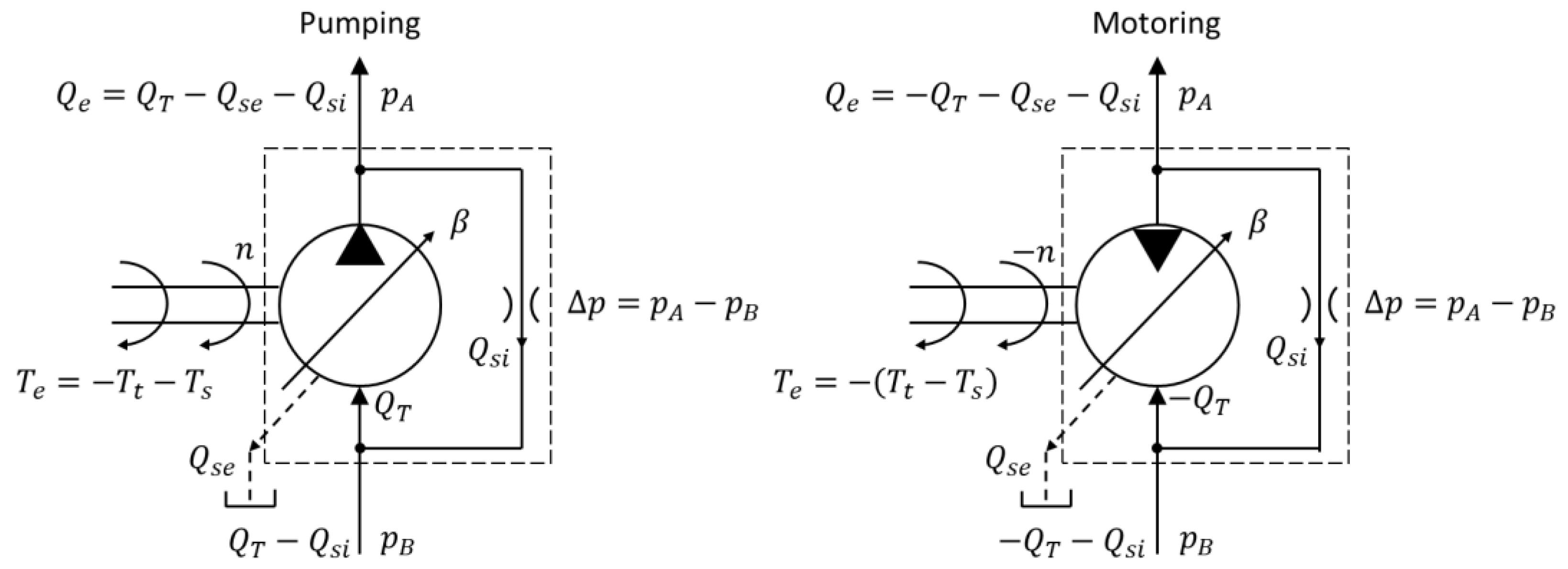
The theoretical flow rate and torque of the hydraulic unit (pump and motors) are represented by Equations (19) and (20). For a realistic calculation, the volumetric loss and the hydromechanical loss must be considered. In this work, the unit loss look-up table is used to accurately model the pumps and motors (Figure 12), as described in the previous Section 2. The effective flow rate ( and torque are computed using Equations (21) and (22). is the unit external and internal leakage flow.
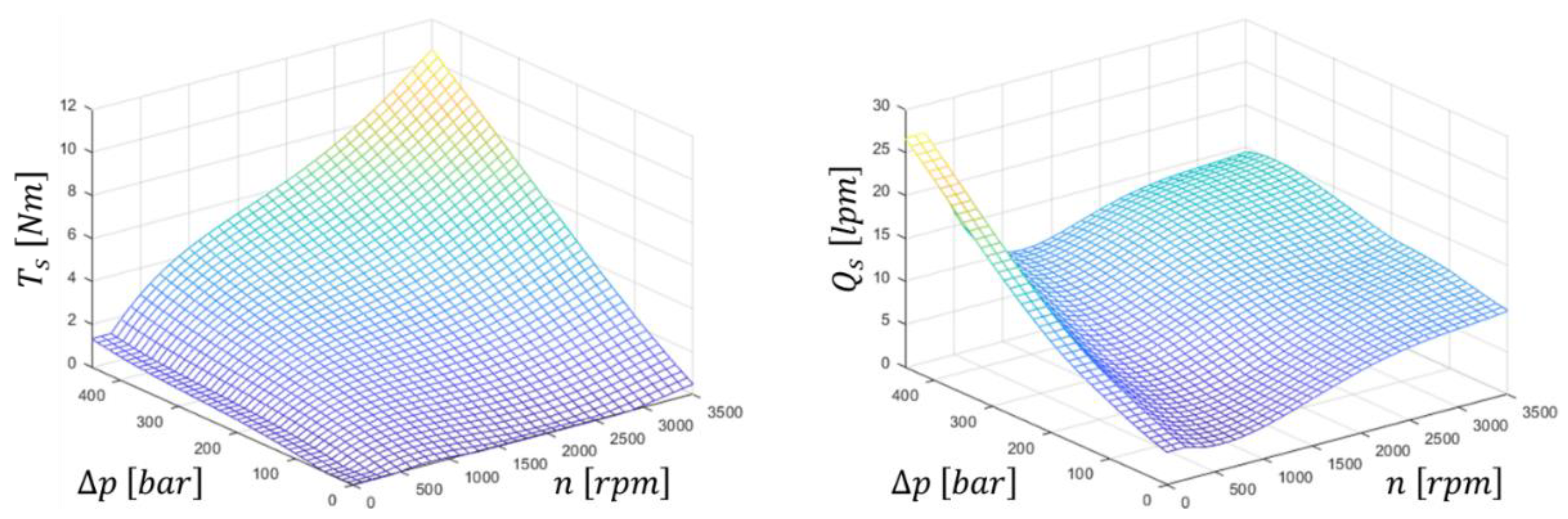
Figure 13 gives an example of the volumetric and hydromechanical loss data from the unit loss look-up table of a 42 cm3/rev swash plate type axial piston pump at 100% displacement. One limitation about the unit loss look-up table is the data may not be available for all the candidate units with different sizes considered in the study. A possible way to solve this problem is to use the linear scaling method to scale a known unit loss look-up table with respect to a certain unit size to a different unit size [31,32,33]. It introduced a linear scaling factor to scale the unit rotational speed, flowrate, and torque as shown in Equations (23)–(26). These loss models are used both in system modeling and sizing optimization.
The scaling approach was used by properly scaling the maps’ input and output of Figure 13.
5.2. Hydraulic Line Capacitance
The pressure build-up Equations (27) and (28) is used to determine the pressure dynamic in line A and line B as a lumped system. This equation is derived from conservation of mass and the constitutive equation for the oil, assuming isothermal conditions [4]. The pressure is directly related to the integration of total flow coming into and out of the control volume and the volume changes . Furthermore, the pressure is proportional to the control volume’s hydraulic capacitance , which include the control volume and bulk modulus . The control volume is calculated based on the hydraulic line inner diameter and the line length. The bulk modulus is chosen based on the oil used in the reference machine and the normal operating temperature.
5.3. Hydraulic Valves
Hydraulic valves such as check valves, relief valves, and on/off valves are modeled as equivalent orifices. Considering that HT does not have a fast–dynamic response affecting system efficiency, the dynamic of these valves is ignored. The flow through an orifice is a function of the valve flow area, which is related to the valve position , an orifice coefficient , the pressure drops and fluid density , as can be seen in Equation (29). The orifice coefficient is empirically found by matching the flow–pressure curves provided by valve manufacturers for the reference vehicle, and the valve position is determined by the controller.
5.4. Machine Dynamic
The machine dynamic includes all the loads applied to the vehicle. Starting from Newton’s second law, the dynamic of the vehicle is described as follows:
All the vehicle information, such as vehicle mass, gear ratio, machine geometry information, rolling resistance, etc. come from the reference machine service manual. is vehicle mass, is vehicle speed, is traction force from the HT, is the load force from the ground, is the gear ratio between the motors to the tracks. The traction force from HT is calculated using the following equation:
Then, the load force is the only unknown. The load force includes air drag, rolling resistant, grading force and resistant force from running over the crop. The following equation is used to describe load force:
As a harvesting machine operates at low velocities, the air drag can be ignored. By comparing the simulated and measured data, the rolling resistance coefficient is chosen to be 0.1 [3]. The only unknown at this point is the resistant force Fr. In practical applications, it can be very challenging to create a reliable model reflecting the complexity of the ground conditions, the unpredictable terrain and crop resistances, also accounting for the weather condition. As an alternative, a back-calculation approach can be used to estimate the resistance force from measurements. In this way, the resulting resistance force can be used as straight input of road resistance in the model. In this way, the vehicle resistance for a given drive cycle can be used to have a fair comparison between the reference and proposed system. The following equations describes the process of back calculation of the resistant force. Rearranging Equations (30)–(32):
In Equation (34), the axle gear , track radius , vehicle mass , rolling resistant coefficient and gravity acceleration are known. The motor torque could be calculated from the measured system pressure and motor displacement. The vehicle speed and pitch angle should be available from measured data. With all these parameters known the resistance force could be easily calculated as the only unknown.
6. Reference HT System and Design Parameters
To prove the concept of the above HT system design method, a heavy-duty harvester is used as a reference machine. The main parameters of the system are shown in Table 2, and the values are close to the values commonly used in large vehicles such as sugar-cane harvesters. The HT system design of the reference machine contains one swashplate type variable displacement axial piston pump and one bent-axis fixed displacement axial piston motor. The power is delivered to the track through a down speed gearbox. There is a shuttle valve for system cooling and a pair of pressure relief valves to protect the system from over pressurization. A charge circuit replenishes the fluid in the system through check valves (Figure 1).
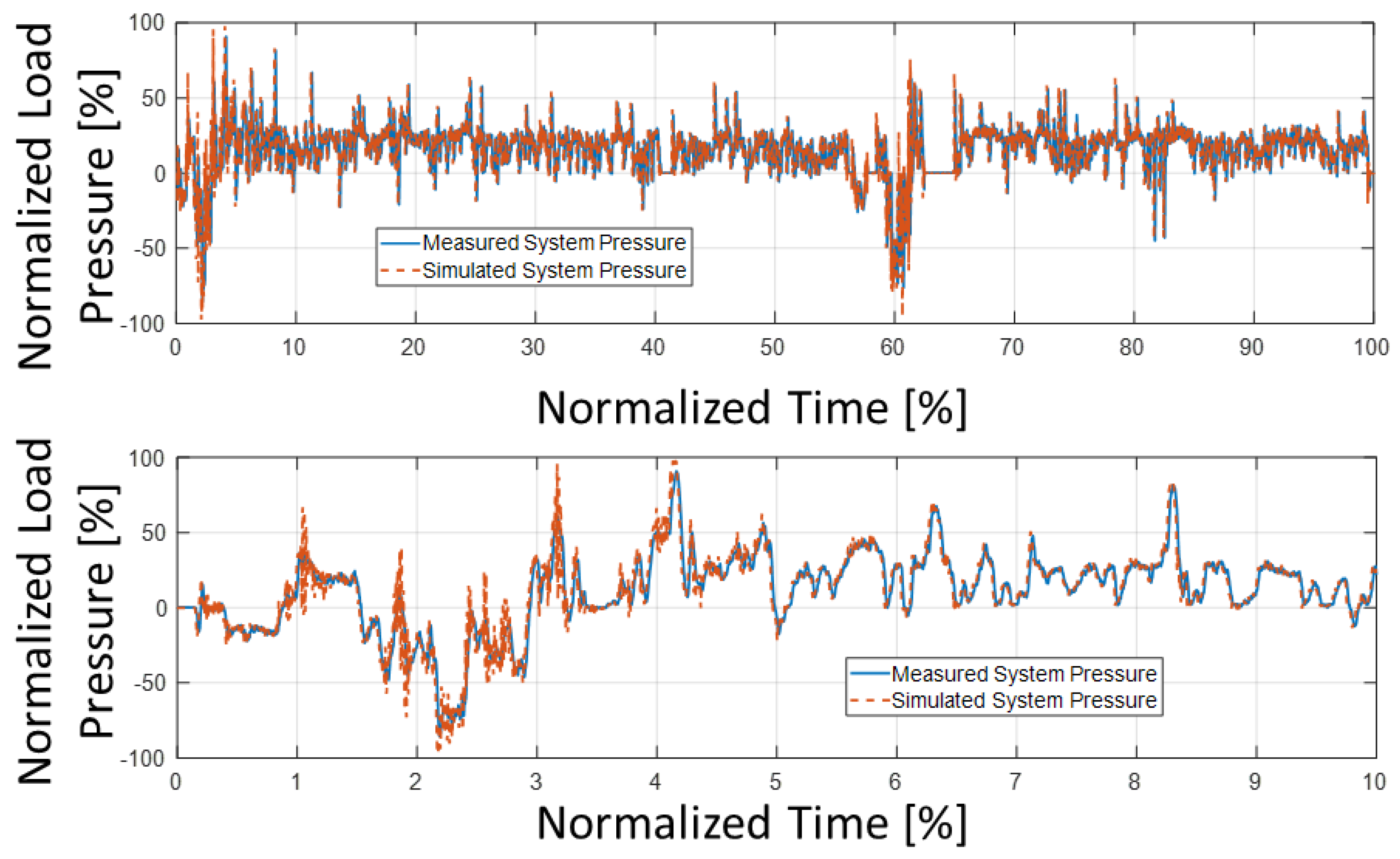
Although detailed vehicle info is not reported here for confidentiality, it is important to note that the model presented in the previous section underwent a detailed validation process by comparing simulation and experimental data. Figure 14 shows an example of comparison between the HT line pressures (normalized) during the reference operating cycle. This comparison showed that the back calculated load force is correctly loading the vehicle in the simulation model for a fair comparison between the different solutions vs. the reference machine. This cycle will be conceptualized for confidentiality and further commented upon in Section 7.
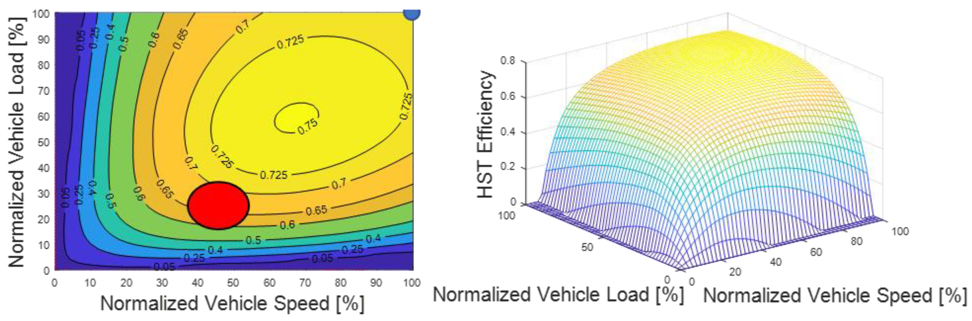
By using Equations (3)–(11), Figure 15 shows the total HT system efficiency plot w.r.t the normalized vehicle full operation range. The plot very clearly shows that the HT system works better at around 70% vehicle speed and 60% vehicle load, which is the best place for the vehicle’s most frequent operating condition. The corner power condition is the blue dot at the upright corner and the most frequent operating condition derived from the drive cycle is around the red circle. It is very clear that the most frequent operating condition are far from the best efficiency point.
Representative Working Condition
The determination of the most frequent operating condition is key in the optimization process. Once the representative working condition is selected, the average load force and speed can be calculated. This information is then used in the evaluation of the objective function.
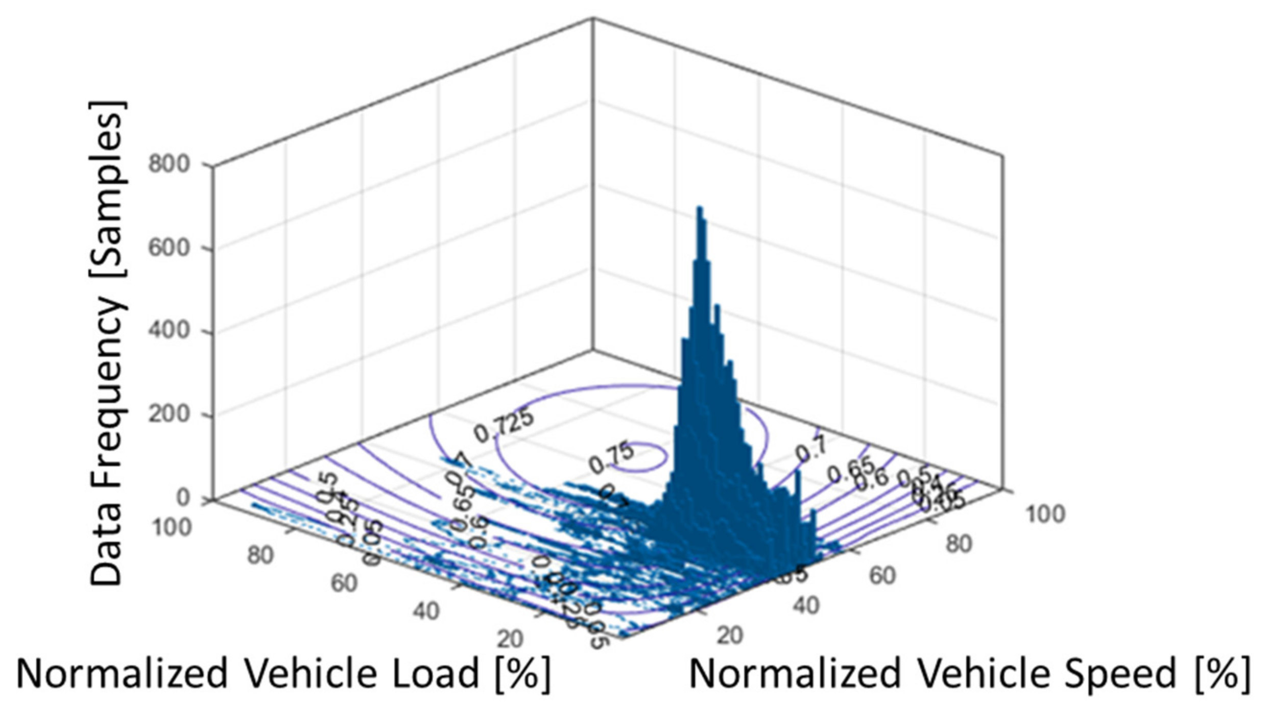
From a sample of measurement data of a commercial harvester, a representative drive cycle is plotted over the HT efficiency map (Figure 16), which shows the speed and load condition throughout the whole drive cycle. Observing the frequency map of the plot gives an idea where the vehicle operates the most. For the reference HT system, the most frequent operating condition was found to be at around 50% of the designed maximum vehicle speed and 25% of designed maximum vehicle load.
7. Results and Discussion
This section discusses the sizing of the alternative architectures, illustrating also how the simulation model can be successfully used for the simulation of an actual HT.
7.1. Model Validation
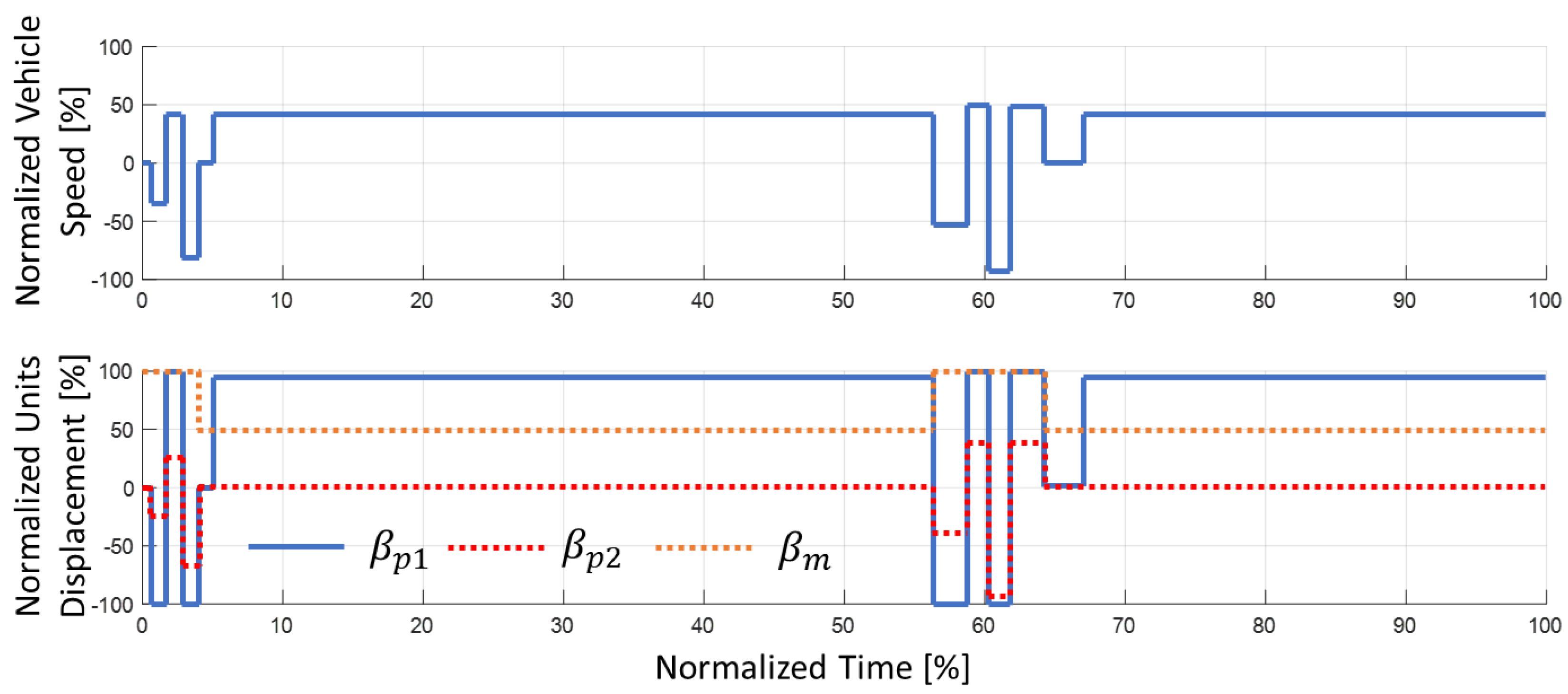
The simulation model was used to reproduce the drive cycle of the reference harvester. A conceptual drive cycle (actual measured data contain confidential data) is shown in Figure 17 top plot. The cycle is formed by a long interval of operation at approximately constant vehicle velocity and load (5–55% and 67–100% of the time). The intervals of constant operation are separated by short maneuvers of the harvester, at changing speed requiring high torque (0–5% and 55–67% of the time). Figure 17 bottom plot shows the units displacement through the drive cycle for reference HT system, which has one variable pump and one fixed motor.
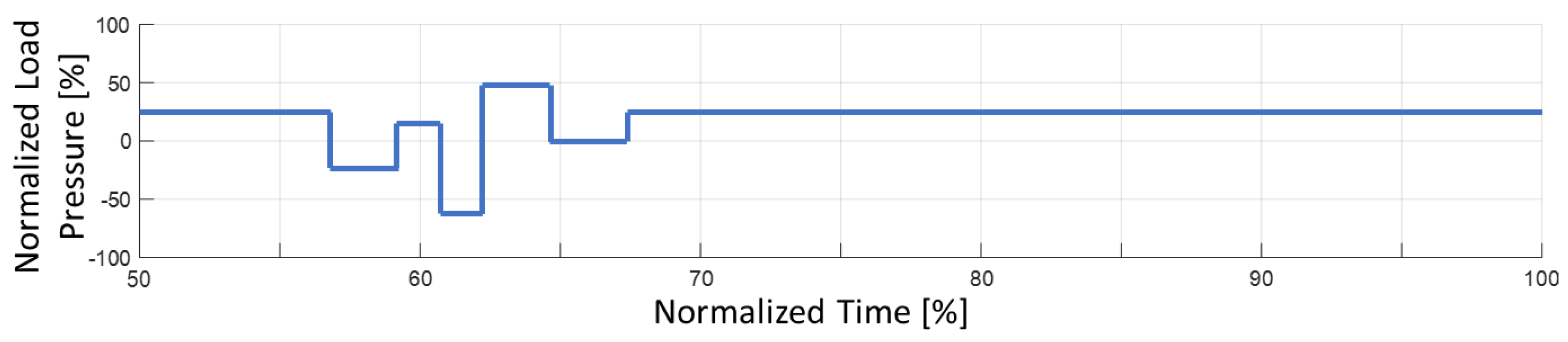
The Figure 18 shows the conceptual normalized load pressure with respect to the same drive cycle as in Figure 17 from 50–100% of the time. The machine had some high load manuver from 55–67% of the time. During 67–100% of the time, the load pressure average is relatively constant at 25%. As the system size optimization is performed w.r.t. constant vehicle speed and load, the effect of the load oscilation is ignored by the optimization process. This means that the efficiency performance improvement found by the optimization procedure will not be reflected exactly in the actual utilization. To quantify this aspect, the simulation model of the vehicle described in Section 5, considering the actual drive cycle, will be utilized.
7.2. Proposed HT System Sizing Optimization
All three Solutions A, B, and C were run through the optimization algorithm to determine the best sizing under the most frequent operating condition. The first five rows of the table show the sizing for the reference machine and the optimal one for the proposed Solutions A, B and C. Then, the “fixed-point optimization” row shows the resulting system efficiency and the percentage power saving of Solutions A, B and C with respect to the reference system, focusing on one fixed operating condition. The last row “drive cycle simulation” shows the system efficiency and percentage power saving of Solutions A, B and C with respect to the reference system, obtained by the simulation model presented in the above section. As this model uses an actual drive cycle, this latter result is more realistic than the fixed-point calculation considered in the optimization.
By observing the results for Solution A, a 49.4% motor displacement as minimum motor setting pushes the system to operate at pressures in the mid to high range, instead of operating at a low pressure as in the reference system. The smaller P1 guarantees that the HT operates near maximum displacement during the most frequent operating condition. The P2 size is relatively large because the system requires achieving maximum speed at maximum force, a condition that is accomplished when the motor is at its maximum displacement.
Solution B (no clutch option) has different optimal sizes for P1 and P2. In this case, P2 always rotates with high hydromechanical losses. As a consequence, the optimal size for P2 is lower with respect to Solution A to limit excessive parasitic losses. As a consequence, P1 has a higher size to meet the flow requirement at full vehicle velocity. Furthermore, at the most frequent operating condition the motor displacement is increased compared to Solution A. This reflects the need for the pump to operate at a higher displacement to promote high HT efficiency.
For Solution C, due to its more limited design freedom, the energy saving is the lowest. The motor has a higher displacement than in Solutions A and B for the same reason illustrated by Solution B: a smaller pump operates at higher displacements, thus promoting higher efficiencies. However, by doing this, Solution C suffers more at low loads. Overall, Solution C provides the worst results in terms of energy savings.
The optimization program predicted the system efficiency and power saving w.r.t, the fixed operation condition which is not realistic in the field. After all the component sizes are determined as shown in Table 3, all solutions are simulated in the realistic drive cycle shown before (Figure 17) through the high-fidelity simulation model to compare their performance and evaluate the effectiveness of the fixed-point optimization procedure. As the real drive cycle is not always at the desired operation condition, the overall system efficiency is lower than the fixed-point calculation, as is expected. However, the three solutions still performed as expected by increasing the system efficiency and providing good power savings.
From the real drive cycle simulation, Solution A gives the best efficiency and saving power. In fact, Solution A has 13.87% efficiency increase and 20.1% total power saving compared to the reference system. Solution B and C also show gains in efficiency (4.36% and 2.15%) and power saving (7.6% and 4.2%) but much less than what Solution A achieved. The reason is because of the compromise made during the system design, such as having no clutch and only one pump. These compromises reduced the design freedom compared to Solution A. As introduced in the introduction, the best working condition for the HT is obtained with the pump at high displacement working at median to high load pressure. Solution A has the design freedom to meet both requirements. However, with the decreased design freedom of Solution B and C, such solutions cannot meet both conditions. What makes it worse is that, with limited design freedom, improving one condition will penalize the other. As a result, the improvements for Solution B and C are very limited.
7.3. Proposed Solution Simulation Results
First, Solution A is simulated using the proposed control logic with same input as the reference system simulation. The results are presented in Figure 19. The sizing of the unit is determined from the optimization above. In the plot showing the unit displacement, the motor changes displacement when the driver changes the driving mode between “high torque” or “working”. In this drive cycle, the driver is in “high torque” mode at first 5% and between 55% and 67% of the normalized time. During these times, the motor was at maximum displacement and both P1 and P2 were working together to provide flow to maintain the vehicle speed. During “working” mode, the motor displacement was at the low position and P2 stopped working. From the bottom plot of Figure 19, the pump was working at higher displacement (>80%) which is also convenient for ensuring high pump efficiency.
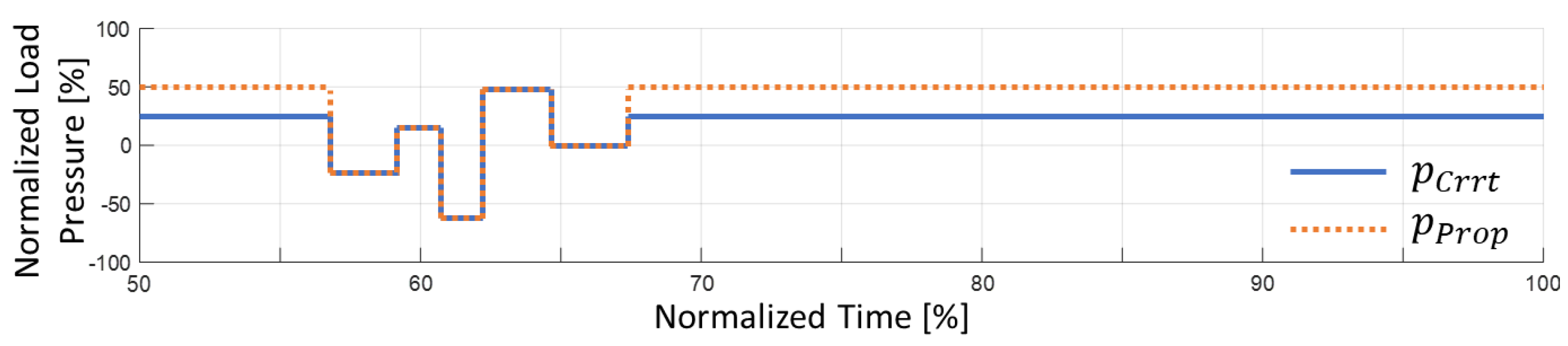
Figure 20 shows the normalized load pressure comparison between the current HT system vs. the Solution A for the same drive cycle. With the two-position motor working at low displacement during the most frequent operation condition, the working pressure was higher than the reference system as designed (~50%), which is more efficient for the both pump and motor.
Finally, the overall system efficiency and total input power are calculated and recorded in these simulations for comparison between the reference system and proposed solutions. More detailed results about efficiency gain and power savings are given in the next section.
7.4. Extended Optimization
The proposed approach can be used for the optimal sizing of HTs considering more operating conditions. As a matter of fact, it is typical that the same harvesting machine is used under different working conditions in terms of vehicle speed or resistive load. To consider this realistic need, the proposed procedure was extended to evaluate the energy saving performance of the different architectures by considering changes of the most frequent operating point. In particular, the procedure was used for finding the minimum motor displacement setting (which is a common feature of all proposed solutions) as a function of the working condition. The maximum displacement for the pumps and the motor remains unchanged. Since all the architectures use a dual setting motor, this setting could be adjusted in the field to reflect the operating condition of the vehicle. Based on the data density plot (Figure 16), the final working condition was chosen to be between 40% to 60% of designed maximum vehicle speed and 10% to 35% of designed maximum vehicle load. This range includes most of the working time.
For the extended optimization study, Table 4, Table 5 and Table 6 show the result for the proposed Solution A, B and C. For all tables, the rows and columns are related to different operating conditions of the reference vehicle. The five rows represent different vehicle speeds, and the six columns represent different vehicle load conditions. For each combination of vehicle speed and load, the corresponding operating condition was fed into the optimization algorithm presented in Section 4 and the optimal motor minimum displacement (Table on the left) and the corresponding efficiency gain vs. the reference machine (Table on the right) was obtained for the corresponding combination. The number in red represents the operation point shown in the above section.
For Solution A, the results are very pleasing with respect to the efficiency gain. The solution can perform quite well and provide high energy efficiency gain over a wide range of working conditions. A clear trend with load can be identified: as the working load increases, the saving decreases. This is because with a higher load, the baseline system working pressure increases bringing the system to operate at higher efficiencies. Similar trends can be noticed on the working speed. For high working speeds, the baseline system pump operates at higher displacement, thus promoting better efficiencies. Therefore, low speeds and low loads are the best working mode to achieve most of the benefits from Solution A.
Solution B also gives good efficiency gain over the whole working range, but the savings are much lower than Solution A. This is because P2 is always in idle condition. The trends previously observed for Solution A are not clearly visible for Solution B. In fact, at 40–45% rated maximum vehicle speed, the saving does not decrease for an increased load. Additionally, for 10–20% rated maximum vehicle load, the saving does not decrease with a vehicle velocity increase. This can be explained considering that in Solution B, P2 always runs in the idle condition, which introduces a relatively constant parasitic loss to the system, causing a significant reduction in efficiency gain at all working conditions. When the total power involved is high (at high speeds and high loads), this loss contributes only a small portion of the total loss, and therefore it reflects moderately on the above. However, when the total power is low (at low velocities and low loads) this greatly reduces efficiency gain because the parasitic loss of P2 became a much greater portion of the total loss. Therefore, the low speed and low load condition is no longer the best operating condition for the HT.
Solution C, on the other hand, shows very little potential compared to the previous solutions. The pump always runs at a partial displacement, bringing much higher volumetric and hydromechanical losses to the system compared to the previous Solutions A and B. Therefore, Solution C saves the most energy with respect to the baseline at high speed, where the pump is at a high displacement setting.
8. Conclusions
Hydrostatic transmission (HT) design and sizing methods discussed in the literature mainly follow methodologies based on the HT corner power condition. This can lead to excessive energy loss when the vehicle operates in normal—the most frequent—operating conditions. In this paper, simple and cost-effective modifications of the basic HT circuit are considered to allow maximizing the energy efficiency while still permitting the transmission to fulfill the vehicle requirements. The main achievements are listed as follows:
- New design solutions are proposed to enable additional regulating freedom by using different combinations of two primary units and a two-displacement motor. These solutions are indicated with the letters A, B, and C.
- The sizing method is based on a genetic algorithm that finds the optimal displacement of the units at the most frequent operating condition of the vehicle.
- An accurate lumped parameter model of the HT system is presented to analyze the performance of each candidate solution under realistic drive cycles.
- The simulation results show how the best solution among the proposed ones can bring to energy efficiency gains of 14% and power savings around 20.1%, when compared to the system taken as initial reference and representative of a commercial solution.
- Furthermore, the paper investigated a method to extend the operating condition with the proposed solutions. By varying the low displacement setting of the hydraulic motor, each one of the proposed solutions can accommodate different operating conditions to ensure maximum energy efficiency.
Author Contributions
Conceptualization, X.G., under the guidance of A.V.; methodology, X.G., under the guidance of A.V.; software, A.V.; validation, X.G.; formal analysis, X.G.; investigation, X.G.; resources, A.V.; data curation, X.G.; writing—original draft preparation, X.G.; writing—review and editing, A.V.; visualization, X.G.; supervision, A.V.; project administration, A.V.; funding acquisition, A.V. All authors have read and agreed to the published version of the manuscript.
Funding
This Research was supported by internal funding of Purdue University available at the Maha Fluid Power Research Center.
Institutional Review Board Statement
Not applicable.
Informed Consent Statement
Not applicable.
Data Availability Statement
The authors exclude this statement.
Conflicts of Interest
The authors declare no conflict of interest.
Nomenclature
| Flow rate | |
| Torque | |
| Rotational Speed | |
| Pressure | |
| Hydraulic Unit Max. Displacement | |
| Hydraulic Unit Displacement | |
| Efficiency | |
| Hydraulic Capacitance | |
| Flow Coefficient | |
| Valve Position | |
| Hydraulic Fluid Density | |
| Bulk Modulus | |
| Volume of the Control Volume | |
| Vehicle Speed | |
| Vehicle Load Force | |
| Gear Ratio | |
| Track Rolling Radius | |
| Air Drag Coefficient | |
| Air Drag Area | |
| Rolling Resistance | |
| Vehicle Mass | |
| Gravitational Acceleration Constant | |
| Road Grading | |
| Subscripts | |
| Pump (Flow/Torque/Speed…) | |
| Motor (Flow/Torque/Speed…) | |
| Theoretical (Flow/Torque) | |
| Effective (Flow/Torque) | |
| Loss (Volumetric/Hydromechanical) | |
| External Volumetric Loss (Pump/Motor) | |
| Internal Volumetric Loss (Pump/Motor) | |
| Engine (Rotational Speed) | |
| Pump Volumetric (Efficiency) | |
| Pump Hydromechanical (Efficiency) | |
| Motor Volumetric (Efficiency) | |
| Motor Hydromechanical (Efficiency) | |
| System Overall (Efficiency) | |
| Resistant Over the Crop (Load Force) | |
| Traction (Load Force) | |
References
- Heywood, J.B. Internal Combustion Engine Fundamentals; McGraw-Hill Education: New York, NY, USA, 2018. [Google Scholar]
- Nervergna, N.; Rundo, M. Passi Nell’oleodinamica; Epics: Torino, TO, Italy, 2020. [Google Scholar]
- Zarotti, G.L. Trasmissioni Idrostatiche. Istituto per le Macchine Agricole e Movimento Terra 2003, 707, 2003. [Google Scholar]
- Vacca, A.; Franzoni, G. Hydraulic Fluid Power: Fundamentals, Applications, and Circuit Design; Wiley: Hoboken, NJ, USA, 2021. [Google Scholar]
- Costa, G.; Sepehri, N. Hydrostatic Transmissions and Actuators: Operation, Modelling and Application; John Wiley & Sons: Hoboken, NJ, USA, 2015. [Google Scholar]
- Paoluzzi, R.; Zarotti, L.G. The Minimum Size of Hydrostatic Transmissions for Locomotion. J. Terramech. 2013, 50, 153–164. [Google Scholar] [CrossRef]
- Ivantysyn, J.; Ivantysynova, M. Hydrostatic Pumps and Motors, Principles, Designs, Performance, Modelling, Analysis, Control and Testing; Academia Books International: New Delhi, India, 2001. [Google Scholar]
- Singh, V.P.; Pandey, A.K.; Dasgupta, K. Steady-state Performance Investigation of Closed-Circuit Hydrostatic Drive Using Variable Displacement Pump and Variable Displacement Motor. Proc. Inst. Mech. Eng. Part E J. Process. Mech. Eng. 2021, 235, 249–258. [Google Scholar] [CrossRef]
- Manring, N.D. Mapping the Efficiency for a Hydrostatic Transmission. J. Dyn. Syst. Meas. Control 2016, 138, 031004. [Google Scholar] [CrossRef]
- Keller, N.; Ivantysynova, M. A New Approach to Sizing Low Pressure Systems. In Proceedings of the In ASME/BATH Symposium on Fluid Power and Motion Control, Sarasota, FL, USA, 16–19 October 2017. [Google Scholar]
- Kress, J.H. Hydrostatic power-splitting transmissions for wheeled vehicles—classification and theory of operation. SAE Trans. 1968, 77, 2282–2306. [Google Scholar]
- Mistry, S.I.; Sparks, G.E. Infinitely Variable Transmission (IVT) of John Deere 7000 TEN Series Tractors. ASME Int. Mech. Eng. Congr. Expo. 2002, 36312, 123–131. [Google Scholar]
- Meyerle, M. Continuous hydrostatic-mechanical branch power split transmission particularly for power vehicles. U.S. Patent 5,683,322, 20 April 1994. [Google Scholar]
- Bottiglione, F.; Mantriota, G.; Valle, M. Power-Split Hydrostatic Transmissions for Wind Energy Systems. Energys 2018, 11, 3369. [Google Scholar] [CrossRef] [Green Version]
- Macor, A.; Rossetti, A. Optimization of Hydro-mechanical Power Split Transmissions. Mech. Mach. Theory 2011, 46, 1901–1919. [Google Scholar] [CrossRef]
- Brusstar, M. Hydraulic Hybrids; U.S. Environmental Protection Agency: Washington, DC, USA, 2006.
- Sprengel, M.; Bleazard, T.; Haria, H.; Ivantysynova, M. Implementation of a Novel Hydraulic Hybrid Powertrain in a Sport Utility Vehicle. In Proceedings of the 2014 IFAC Workshop on Engine and Powertrain Control, Simulation and Modeling, Columbus, OH, USA, 23–26 August 2015. [Google Scholar]
- Kumar, R.; Ivantysynova, M. The Hydraulic Hybrid Alternative for Toyota Prius—A Power Management Strategy for Improved Fuel Economy. In Proceedings of the 7th International Fluid Power Conference (7. IFK), Aachen, Germany, 22–24 March 2010. [Google Scholar]
- Kumar, R.; Ivantysynova, M. An Optimal Power Management Strategy for Hydraulic Hybrid Output Coupled Power-Split Transmission. In Proceedings of the ASME 2009 Dynamic Systems and Control Conference, Hollywood, CA, USA, 12–14 October 2009; 1, pp. 229–306. [Google Scholar]
- Kumar, R.; Ivantysynova, M. An instantaneous Optimization Based Power Management Stratege to Reduce Fuel Consumption in Hydraulic Hybrids. Int. J. Fluid Power 2011, 12, 15–25. [Google Scholar] [CrossRef]
- Heikkilä, M.; Huova, M.; Tammisto, J.; Linjama, M.; Tervonen, J. Fuel Efficiency Optimization of a Baseline Wheel Loader and its Hydraulic Hybrid Variants Using Dynamic Programming. In Proceedings of the BATH/ASME 2018 Symposium on Fluid Power and Motion Control, Bath, UK, 12–14 September 2018. [Google Scholar]
- Sprengel, M.; Ivantysynova, M. Neural Network Based Power Management of Hydraulic Hybrid Vehicles. Int. J. Fluid Power 2017, 18, 79–91. [Google Scholar] [CrossRef]
- Cheong, K.L.; Li, P.Y.; Chase, T.R. Optimal Design of Power-Split Transmissions for Hydraulic Hybrid Passenger Vehicles. In Proceedings of the 2011 American Control Conference, San Francisco, CA, USA, 29 June–1 July 2011. [Google Scholar]
- Paoluzzi, R.; Zarotti, L.G. Properties and sizing methods of 2-motor transmissions. Int. J. Fluid Power 2017, 18, 3–16. [Google Scholar] [CrossRef]
- Stump, P.M.; Keller, N.; Vacca, A. Energy Management of Low-Pressure Systems Utilizing Pump-Unloading Valve and Accumulator. Energies 2019, 12, 4423. [Google Scholar] [CrossRef] [Green Version]
- Pelosi, M.; Ivantysynova, M. A Geometric Multigrid Solver for the Piston-Cylinder Interface of Axial Piston Machines. Tribol. Trans. 2012, 55, 163–174. [Google Scholar] [CrossRef]
- Chen, Y.; Zhang, J.; Xu, B.; Chao, Q.; Liu, G. Multi-objective Optimization of Micron-Scale Surface Textures for the Cylinder/Valve Plate Interface in Axial Piston Pumps. Tribol. Int. 2019, 138, 316–329. [Google Scholar] [CrossRef]
- Golberg, D.E. Genetic Algorithms in Search, Optimization, and Machine Learning; Addion Wesley: Boston, MA, USA, 1989. [Google Scholar]
- Frank, M.; Drikakis, D.; Vharissis, V. Machine-Learning Methods for Computational Science and Engineering. Computation 2020, 8, 15. [Google Scholar] [CrossRef] [Green Version]
- Nelder, J.A.; Mead, R. A Simplex Method for Function Minimization. Comput. J. 1965, 7, 308–313. [Google Scholar] [CrossRef]
- Shang, L.; Ivantysynova, M. An Investigation of Design Parameters Influencing the Fluid Film Behavior in Scaled Cylinder Block/Valve Plate Interface. In Proceedings of the 9th FPNI Ph.D. Symposium on Fluid Power, Florianópolis, SC, Brazil, 26–28 October 2016. [Google Scholar]
- Shang, L.; Ivantysynova, M. A Path Toward Effective Piston/Cylinder Interface Scaling Approach. In Proceedings of the ASME/BATH 2017 Symposium on Fluid Power and Motion Control, Sarasota, FL, USA, 16–19 October 2017. [Google Scholar]
- Shang, L.; Ivantysynova, M. Scaling Criteria for Axial Piston Machines Based on Thermo-Elastohydrodynamic Effects in the Tribological Interfaces. Energies 2018, 11, 3210. [Google Scholar] [CrossRef] [Green Version]
Figure 1.
Typical Closed Loop Hydrostatic Transmission Circuit.

Figure 2.
Reference HT System Operation Condition.

Figure 3.
Transmission Schematic for Proposed Solution A.

Figure 4.
HT Operating Range: Reference (Left) vs. Solution A (Right).

Figure 5.
Transmission Schematic for Proposed Solution B.

Figure 6.
Transmission Schematic for Proposed Solution C.

Figure 7.
HT Operating Range: Reference (Left) vs. Solution C (Right).

Figure 8.
Control Block Diagram for the HT Solution A and B.

Figure 9.
Pump and Motor Control near the Most Frequent Operating Condition.

Figure 10.
Pump and Motor Control for Solution A and B—High Torque Mode.

Figure 11.
Transmission Block Diagram.

Figure 12.
Pump/Motoring Model.

Figure 13.
Volumetric (Left) and Hydromechanical (Right) Loss Model.

Figure 14.
Measured vs. Simulated Normalized Load Pressure (Up is Full Drive Cycle; the lower image is Zoomed in for the First 10% of the time).
Figure 14.
Measured vs. Simulated Normalized Load Pressure (Up is Full Drive Cycle; the lower image is Zoomed in for the First 10% of the time).

Figure 15.
HT System Efficiency Map Data (Left) and HT System Efficiency Map (Right).

Figure 16.
Frequency Representative of the Instances of Vehicle Operation in the HT Efficiency Map—Reference System.
Figure 16.
Frequency Representative of the Instances of Vehicle Operation in the HT Efficiency Map—Reference System.

Figure 17.
Conceptual Drive Cycle of Vehicle Speed and Unit Displacement.

Figure 18.
Conceptual Drive Cycle of Vehicle Load at 50–100% of the Time.

Figure 19.
Simulation results (Solution A).

Figure 20.
Normalized motor load. Comparison between the Standard system vs. Solution A.


Table 1.
Design Variables and Range.
| Variables | Representation | Variable Pool | Bits |
|---|---|---|---|
| P1 Max. Displacement | |||
| P2 Max. Displacement | |||
| Motor Max. Displacement | |||
| Motor Working Displacement |
Table 2.
Important HT Design Parameters.
| Variables | Value | Units | Description |
|---|---|---|---|
| 2500 | rpm | Pump Rotational Speed | |
| 100 | cc/rev | Pump Maximum Displacement | |
| 80 | cc/rev | Motor Maximum Displacement | |
| 100 | % | Normalized Maximum Vehicle Speed | |
| 56 | % | Normalized Most Frequent Vehicle Speed | |
| 100 | % | Normalized Maximum Load Torque on Motor | |
| 20 | % | Normalized Most Frequent Load Torque on Motor | |
| 400 | bar | Maximum Working Pressure | |
| 50 | - | Gear Ratio from Motor to Track | |
| 0.40 | m | Track Rolling Radius |
Table 3.
Optimization result sizing for the Proposed HT.
| Reference | Solution A | Solution B | Solution C | ||
|---|---|---|---|---|---|
| [cc/rev] | 100 | 28 | 45 | 100 | |
| [cc/rev] | 0 | 75 | 55 | 0 | |
| [cc/rev] | 80 | 80 | 80 | 80 | |
| [%] | 100 | 49.4 | 56.4 | 69.4 | |
| Clutch | No | Yes | No | No | |
| Fixed Point Optimization | System Eff. [%] | 62.23 | 78.88 | 69.98 | 63.49 |
| Pwr. Saving [%] | - | 21.10 | 11.07 | 2.00 | |
| Drive Cycle Simulation | System Eff. [%] | 55.81 | 69.68 | 60.17 | 57.96 |
| Pwr. Saving [%] | - | 20.11 | 7.57 | 4.22 | |
Table 4.
Optimal Motor Displacement and Efficiency Gain for Expand Working Conditions (Solution A). (The number in red represents the operation point shown in the above section).
Table 4.
Optimal Motor Displacement and Efficiency Gain for Expand Working Conditions (Solution A). (The number in red represents the operation point shown in the above section).
| Motor Beta Map [%] | Vehicle Load [%] | Efficiency Gain [%] | Vehicle Load [%] | ||||||||||||
|---|---|---|---|---|---|---|---|---|---|---|---|---|---|---|---|
| 10 | 15 | 20 | 25 | 30 | 35 | 10 | 15 | 20 | 25 | 30 | 35 | ||||
| Vehicle Speed [%] | 60 | 39.1 | 42.2 | 44.9 | 44.9 | 44.9 | 44.9 | Vehicle Speed [%] | 60 | 24.4 | 17.7 | 13.2 | 9.9 | 7.0 | 4.4 |
| 55 | 42.0 | 45.1 | 48.1 | 49.4 | 49.4 | 49.4 | 55 | 24.2 | 18.1 | 14.1 | 11.2 | 8.8 | 6.6 | ||
| 50 | 45.1 | 48.5 | 51.6 | 54.6 | 54.9 | 54.9 | 50 | 24.2 | 18.7 | 15.1 | 12.7 | 10.7 | 9.0 | ||
| 45 | 48.5 | 52.5 | 55.9 | 59.1 | 61.8 | 61.8 | 45 | 24.3 | 19.4 | 16.2 | 14.3 | 12.8 | 11.5 | ||
| 40 | 52.2 | 57.4 | 61.3 | 64.8 | 68.0 | 70.6 | 40 | 24.4 | 20.1 | 17.5 | 16.1 | 15.0 | 14.2 | ||
Table 5.
Optimal motor displacement and efficiency gain for different working conditions (Solution B).The number in red represents the operation point shown in the above section.
Table 5.
Optimal motor displacement and efficiency gain for different working conditions (Solution B).The number in red represents the operation point shown in the above section.
| Motor Beta Map [%] | Vehicle Load [%] | Efficiency Gain [%] | Vehicle Load [%] | ||||||||||||
|---|---|---|---|---|---|---|---|---|---|---|---|---|---|---|---|
| 10 | 15 | 20 | 25 | 30 | 35 | 10 | 15 | 20 | 25 | 30 | 35 | ||||
| Vehicle Speed [%] | 60 | 45.1 | 51.2 | 56.3 | 60.5 | 64.3 | 68.5 | Vehicle Speed [%] | 60 | 11.7 | 8.4 | 6.7 | 5.6 | 4.9 | 4.3 |
| 55 | 46.4 | 53.4 | 59.3 | 63.9 | 68.1 | 71.9 | 55 | 10.5 | 7.8 | 6.4 | 5.8 | 5.4 | 5.1 | ||
| 50 | 47.6 | 55.6 | 62.6 | 68.1 | 72.8 | 77.0 | 50 | 9.5 | 7.2 | 6.2 | 6.0 | 5.9 | 6.0 | ||
| 45 | 48.7 | 57.6 | 66.5 | 73.5 | 79.1 | 84.1 | 45 | 8.4 | 6.7 | 6.1 | 6.3 | 6.6 | 7.0 | ||
| 40 | 40.0 | 59.7 | 71.0 | 81.6 | 91.2 | 99.8 | 40 | 7.5 | 6.1 | 6.0 | 6.8 | 7.6 | 8.5 | ||
Table 6.
Optimal motor displacement and efficiency gain for different working conditions (Solution C). The number in red represents the operation point shown in the above section.
Table 6.
Optimal motor displacement and efficiency gain for different working conditions (Solution C). The number in red represents the operation point shown in the above section.
| Motor Beta Map [%] | Vehicle Load [%] | Efficiency Gain [%] | Vehicle Load [%] | ||||||||||||
|---|---|---|---|---|---|---|---|---|---|---|---|---|---|---|---|
| 10 | 15 | 20 | 25 | 30 | 35 | 10 | 15 | 20 | 25 | 30 | 35 | ||||
| Vehicle Speed [%] | 60 | 47.2 | 58.4 | 66.5 | 73.9 | 80.9 | 87.9 | Vehicle Speed [%] | 60 | 6.2 | 2.6 | 0.7 | 0.1 | 0 | 0.2 |
| 55 | 49.1 | 61.0 | 69.9 | 78.4 | 87.6 | 100 | 55 | 5.1 | 1.9 | 0.4 | 0 | 0.1 | 0.6 | ||
| 50 | 51.3 | 61.3 | 74.1 | 85.3 | 100 | 100 | 50 | 4.0 | 1.4 | 0.1 | 0.1 | 0.6 | 1.2 | ||
| 45 | 53.9 | 64.7 | 80.2 | 100 | 100 | 100 | 45 | 3.0 | 0.8 | 0 | 0.5 | 1.2 | 1.9 | ||
| 40 | 57.2 | 69.0 | 100 | 100 | 100 | 100 | 40 | 2.0 | 0.3 | 0.1 | 1.2 | 1.9 | 2.5 | ||
Publisher’s Note: MDPI stays neutral with regard to jurisdictional claims in published maps and institutional affiliations. |
© 2021 by the authors. Licensee MDPI, Basel, Switzerland. This article is an open access article distributed under the terms and conditions of the Creative Commons Attribution (CC BY) license (https://creativecommons.org/licenses/by/4.0/).
Share and Cite
MDPI and ACS Style
Guo, X.; Vacca, A. Advanced Design and Optimal Sizing of Hydrostatic Transmission Systems. Actuators 2021, 10, 243. https://0-doi-org.brum.beds.ac.uk/10.3390/act10090243
AMA Style
Guo X, Vacca A. Advanced Design and Optimal Sizing of Hydrostatic Transmission Systems. Actuators. 2021; 10(9):243. https://0-doi-org.brum.beds.ac.uk/10.3390/act10090243
Chicago/Turabian StyleGuo, Xiaofan, and Andrea Vacca. 2021. "Advanced Design and Optimal Sizing of Hydrostatic Transmission Systems" Actuators 10, no. 9: 243. https://0-doi-org.brum.beds.ac.uk/10.3390/act10090243
Note that from the first issue of 2016, this journal uses article numbers instead of page numbers. See further details here.