Fault-Tolerant Control of a Three-Phase Permanent Magnet Synchronous Motor for Lightweight UAV Propellers via Central Point Drive

Abstract

This paper deals with the development and the performance characterization of a novel Fault-Tolerant Control (FTC) aiming to the diagnosis and accommodation of electrical faults in a three-phase Permanent Magnet Synchronous Motor (PMSM) employed for the propulsion of a modern lightweight fixed-wing UAV. To implement the fault-tolerant capabilities, a four-leg inverter is used to drive the reference PMSM, so that a system reconfiguration can be applied in case of a motor phase fault or an inverter fault, by enabling the control of the central point of the three-phase connection. A crucial design point is to develop Fault-Detection and Isolation (FDI) algorithms capable of minimizing the system failure transients, which are typically characterized by high-amplitude high-frequency torque ripples. The proposed FTC is composed of two sections: in the first, a deterministic model-based FDI algorithm is used, based the evaluation of the current phasor trajectory in the Clarke’s plane; in the second, a novel technique for fault accommodation is implemented by applying a reference frame transformation to post-fault commands. The FTC effectiveness is assessed via detailed nonlinear simulation (including sensors errors, digital signal processing, mechanical transmission compliance, propeller loads and electrical faults model), by characterizing the FDI latency and the post-fault system performances when open circuit faults are injected. Compared with reports in the literature, the proposed FTC demonstrates relevant potentialities: the FDI section of the algorithm provides the smallest ratio between latency and monitoring samples per electrical period, while the accommodation section succeeds in both eliminating post-fault torque ripples and maintaining the mechanical power output with negligible efficiency degradation.

1. Introduction

1.1. Research Context

The global market of Unmanned Aerial Vehicles (UAVs), despite the dramatic economic consequences of the COVID-19 pandemic, is estimated to reach USD 27.4 billion in 2021, and it is projected to increase to USD 58.4 billion by 2026 at a compound annual growth rate of 16.4% [1]. In addition, the increasing demand of ecofriendly air operations is driving the design of next generation long-endurance UAVs to electrically powered propulsion solutions. Though still immature, full-electric technologies are expected to obtain large investments in the near future, up to replace conventional Internal Combustion Engine (ICE), as well as hybrid or hydrogen-based solutions [2]. Full-electric propulsion systems would actually assure lower CO₂-emissions, lower noise, smaller thermal signature (for military applications), higher efficiency, and simplified maintenance [3]. Nevertheless, several reliability and safety issues are still open, especially for long-endurance UAVs flying in unsegregated airspaces. In particular, architectures based on three-phase Permanent Magnets Synchronous Machines (PMSM) with conventional inverters are vulnerable to fault modes with high failure rates (ranging from 100 to 200 per million flight hours [4]), such as the open-transistor, open-phase, phase-to-leg short-circuit, transistor short-circuit or capacitor short-circuit [5]. Typically, motor phase faults and inverter faults cover from 60% to 70% of the PMSM fault modes [6], and the related post-fault behaviour is characterised by relevant torque oscillations [7,8] with potential unsafe operation.

Provided that the lightweight and compactness requirements for UAVs impede the extensive use of hardware redundancy (e.g., redundant motors), the reliability enhancement of full-electric propulsion systems is typically achieved by motor phase redundancy or unconventional inverters. Different redundant architectures are proposed in the literature: motors with redundant phases [9,10], motors with multiple three-phase arrangements [11,12], phase-isolating inverters [6,11,12], but a relevant increase of weight is typically obtained. An alternative solution (which this work refers to) can be obtained by using a standard three-phase PMSM driven by a four-leg inverter [13,14], in which a couple of power switches are included, as stand-by devices, in the inverter. In case of electrical faults, the stand-by switches are activated to control the central point of the three-phase connection, Figure 1.

Independent from the selection of hardware redundancy solution, a crucial design point is always related the development of appropriate Fault-Detection and Isolation (FDI) algorithms; actually, the electrical faults, especially for PMSMs operating at high speeds, imply the generation of high-amplitude high-frequency torque ripples, and failure transients can cause potentially unsafe conditions if FDI latency is not adequately small.

1.2. Motivation of the Research

Many research activities have been developed in recent years on FDI of PMSM electrical faults. Kontarček [15] and Saleh [16] proposed predictive methods, relying on the stator current prediction and estimation error. Though the methods assure extremely small latencies, their robustness depends on the availability of an extensive database of electric parameters as functions of environment and aging. A fault diagnosis for open-phase faults using an extended Kalman filter is proposed in [17], while a FDI method based on residual generation is realized in [18], by elaborating RMS values and direct measurements of phase currents. Jun [19] presented a phase faults detection by performing the power spectrum analysis of the Zero Sequence Voltage Component (ZSVC) signal, but no direct discrimination between internal stator winding faults and inverter faults is obtained, so additional sensors and analysis are implemented to isolate the fault via recursive technique. Khalaief [7] and Huang [20] implemented the FDI by merging a Fast Fourier Transform (FFT) of the current signals with a model-based Current Signature (CS) technique, in order to first detect the stator phase fault and then to isolate the failed phase. The basic idea of the CS technique is that the trajectory of the current phasor in the Clarke plane can be correlated with the operative state of the three-phase system (normal, with open-phase, with short-circuit, etc.). The technique exhibits very good FDI performances, but the relevant limitations derive from the use of FFT analysis, since it requires the monitoring of the stator currents after the fault for an entire (or even more) electrical cycle to perform the detection. Similarly, Peuget [21] carried out the FDI by adopting CS technique, by using the phasor Current Signature Derivative (CSD) as a diagnostic signal, but noise concerns limit the application of this strategy. Other techniques are proposed and validated in [22,23], based on the calculation of a normalized Absolute Average Value (AAV) of the current measurements. The method is simple and robust with respect to torque or speed variations, but it requires a very high monitoring frequency to achieve small FDI latencies.

Concerning the post-fault accommodation, different techniques are proposed by literature. The Rotor Current Feed-Forward (RCFFC) technique [24,25,26] allows to obtain negligible torque degradation in terms of steady-state value, but the control laws robustness is poor. More robust approaches are applied in [25,26], where Stator or Rotor Currents Hysteresis Control techniques (SCHC or RCHC, respectively) are applied. A Rotor Current Frame Transformation Control (RCFTC) is instead proposed in [27,28]: the technique is innovative, and it is based on a standard PI regulator applied to control the motor currents in a reconfigured rotating reference frame, which restores the post-fault AC currents into DC variables. Very good performances are obtained, but further investigations are needed to substantiate the approach.

This work aims to provide a contribution to this research context by developing an innovative FTC devoted to the FDI and accommodation of electrical faults in high-speed PMSMs. The proposed FTC is composed of two sections: the first addresses the FDI problem through a novel approach, using a CS technique without derivative operators (Current Signature no-Derivative, CSnD). No additional measurements with respect to conventional PMSM architectures are used, and no frequency-domain analyses are performed for FDI purposes. The second section of the FTC operates the accommodation of faults, and it is developed by applying the RCFTC technique in order to guarantee enhanced post-fault performances.

The paper is articulated as follows. The first part is dedicated to the nonlinear modelling of the propulsion system; successively, the algorithms for the FDI and the accommodation of faults are described and the basic design criteria are presented and discussed. Finally, a summary of simulation results is proposed, by characterizing the failure transients related to open-phase faults injection. The simulation demonstrates that the FTC developed succeeds in detecting, isolating and accommodating open-phase faults, with negligible degradation of performance in terms of torque, speed and power efficiency, and with more efficient monitoring capabilities with respect to results reported in the literature.

2. Materials and Methods

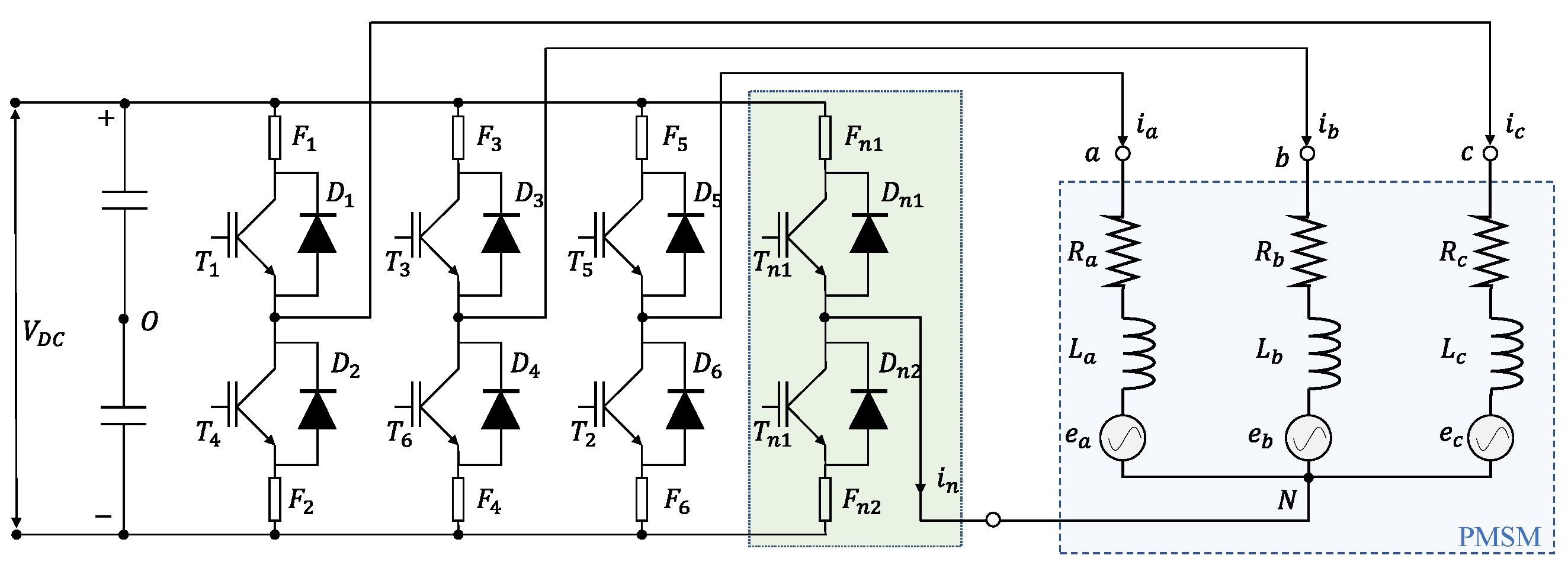
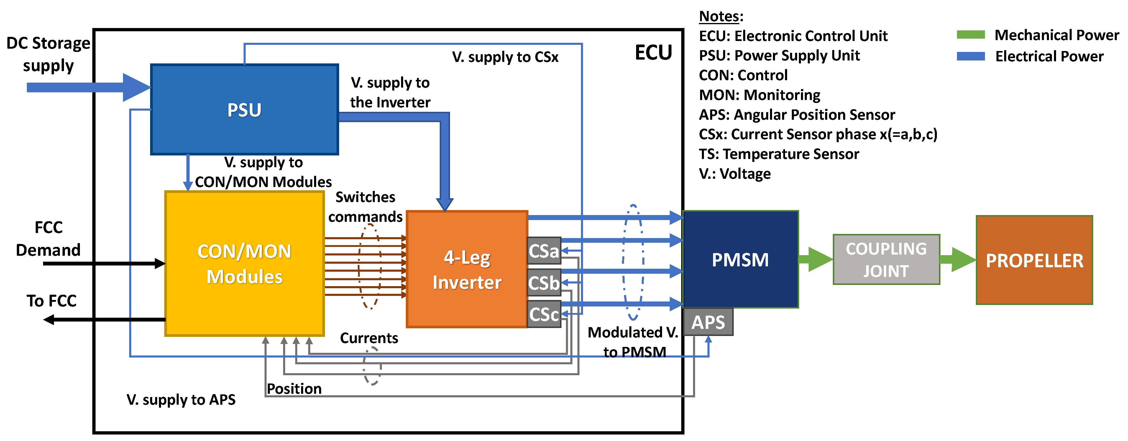
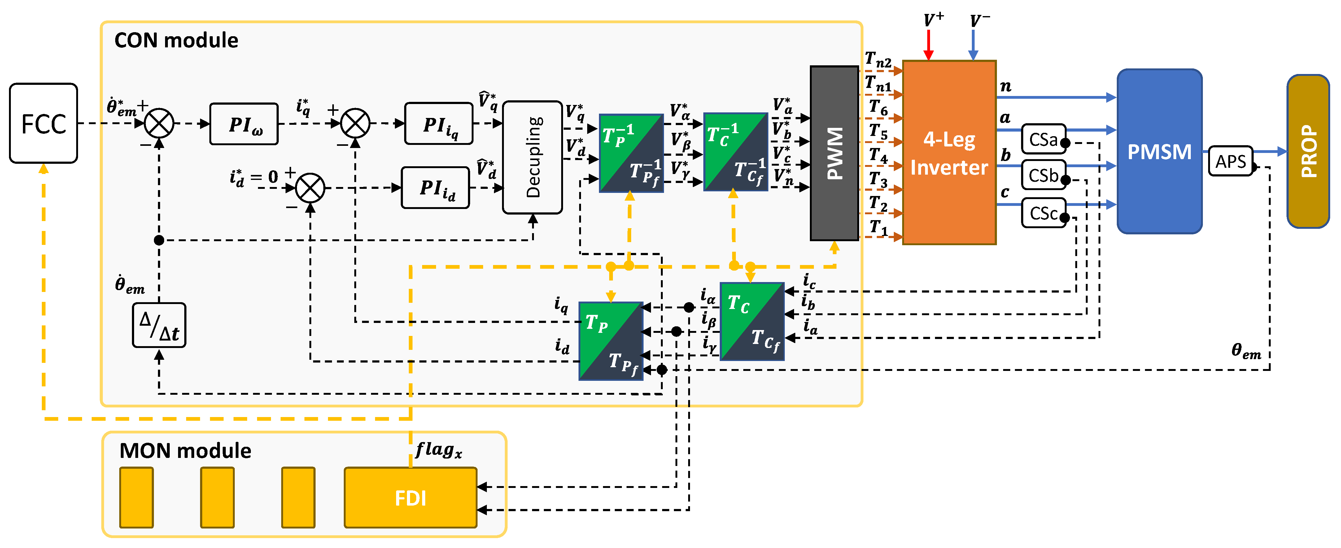
2.1. System Description

The reference system, employed for the full-electric propulsion of a lightweight fixed-wing UAV, is basically composed of (Figure 2):

➢

An electromechanical section, with:

○

Three-phase PMSM, with surface-mounted magnets and phases in Y connection;

○

Twin fixed-pitch propeller (APC22x10E [29]);

○

Mechanical coupling joint.

➢

An Electronic Control Unit (ECU), including:

○

Control/monitoring (CON/MON) module, for the implementation of the closed-loop control and health-monitoring functions;

○

Motor inverter with four-leg architecture;

○

Three Current Sensors (CSa, CSb, CSc), one per each motor phase;

○

Angular Position Sensor (APS), measuring the motor angle;

○

Power Supply Unit (PSU), converting the 48 V_DC input coming from the UAV energy storage system for all components and sensors.

The CON module operates the closed-loop control of the system by implementing two nested loops, on the propeller speed and motor currents (via Field-Oriented Control, FOC). All the regulators implement proportional/integral actions on tracking error signals, plus an anti-windup function with a back-calculation algorithm to compensate for commands saturation. The MON module executes the health-monitoring algorithms, including the FTC proposed in this work.

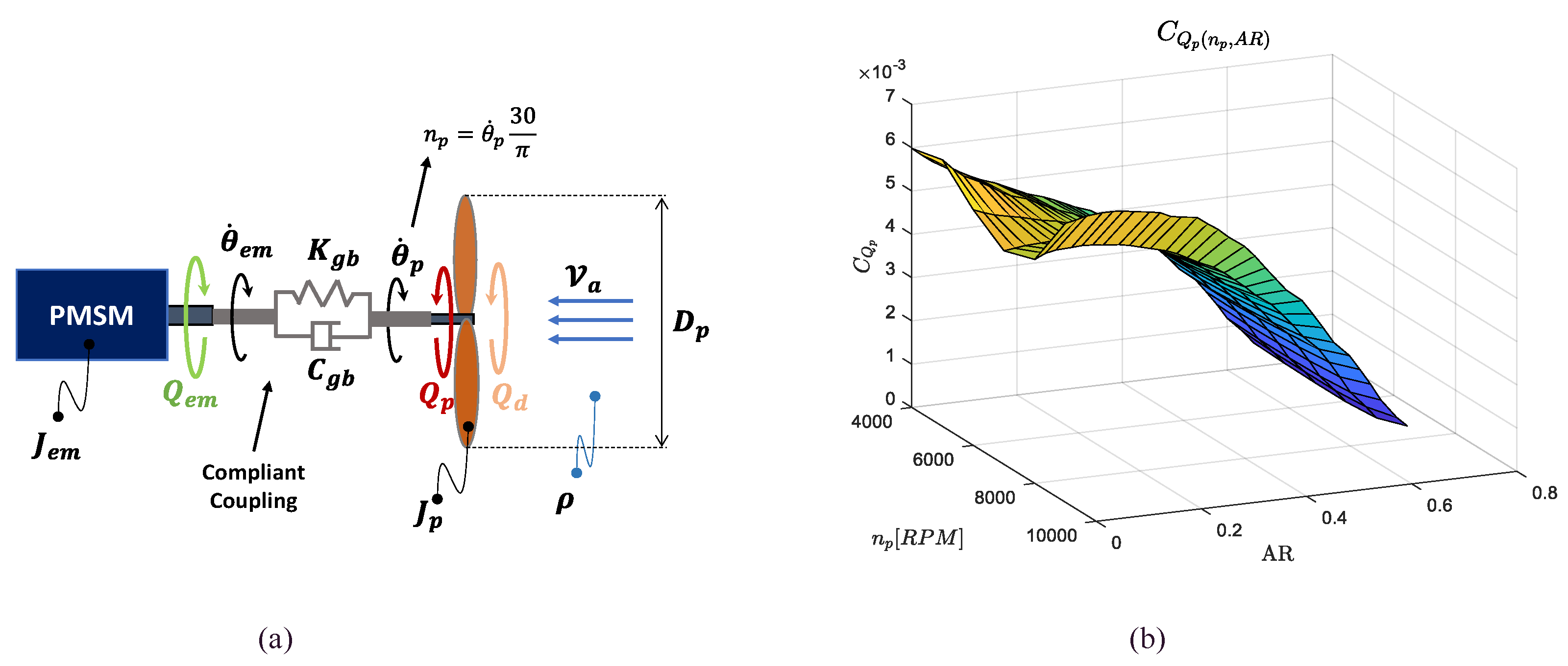
2.2. Aerodynamic and Mechanical Section Modelling

With reference to the scheme depicted in Figure 3a, the dynamics of the mechanical section is modelled via Equation (1) [2]:

$$\{\begin{array}{c}{J}_p{\ddot{\theta }}_p=-Q_p-C_{gb}\left({\dot{\theta }}_p-{\dot{\theta }}_{em}\right)-K_{gb}\left({\theta }_p-{\theta }_{em}\right)+Q_d\\ J_{em}{\ddot{\theta }}_{em}=Q_{em}+C_{gb}\left({\dot{\theta }}_p-{\dot{\theta }}_{em}\right)+K_{gb}\left({\theta }_p-{\theta }_{em}\right)\\ Q_p=C_{Q_p}\left({\dot{\theta }}_p,AR\right)\rho D_p^5{\dot{\theta }}_p^2 \\ AR=\frac{{\mathcal{V}}_a}{D_p{\dot{\theta }}_p}\end{array},$$

(1)

where $J_p$ and $J_{em}$, and ${\theta }_p$ and ${\theta }_{em}$ are the propeller and motor inertias and angles, $Q_d$ is gust-induced disturbance torque, $Q_p$ is the propeller resistant torque, $Q_{em}$ is the motor torque, $C_{Q_p}$ is the nondimensional torque coefficient (Figure 3b), $AR$ is the propeller advance ratio, $D_p$ is the propeller diameter, $\rho$ is the air density and ${\mathcal{V}}_a$ is the UAV forward speed, while $K_{gb}$ and $C_{gb}$ are the stiffness and the damping of the mechanical coupling joint.

2.3. PMSM Modelling

The PMSM dynamics is modelled with reference to the schematics in Figure 4, under the following assumptions [12]:

• Negligible magnetic nonlinearities of ferromagnetic parts (i.e., hysteresis, saturation);
• The motor is magnetically symmetric with respect to its phases;
• The permanent magnets are surface-mounted and made of rare-earth materials—the magnet reluctance along the quadrature axis is infinite with respect to the one along the direct axis;
• Negligible magnetic coupling among phases;
• Negligible reluctances of ferromagnetic parts;
• Negligible magnetic flux dispersion (i.e., secondary magnetic paths, iron losses).

The phase current dynamics in vector form is given by:

$${\mathit{V}}_{abc}=R{\mathit{i}}_{abc}+L\frac{d}{dt}{\mathit{i}}_{abc}+{\mathit{e}}_{abc},$$

(2)

$${\mathit{e}}_{abc}={\lambda }_m{n}_d{\dot{\theta }}_{em}{\left[\sin \left(n_d{\theta }_{em}\right), \sin \left(n_d{\theta }_{em}-\frac{2}{3}\pi \right), \sin \left(n_d{\theta }_{em}+\frac{2}{3}\pi \right)\right]}^T,$$

(3)

where ${\mathit{V}}_{abc}={\left[V_a-V_n,V_b-V_n,V_c-V_n\right]}^T$ is the applied voltage vector, ${\mathit{i}}_{abc}={\left[i_a, i_b, i_c\right]}^T$ is the stator current vector, ${\mathit{e}}_{abc}$ is the back-electromotive force vector, $R$ and $L$ are the resistance and inductance of the motor phases, ${\lambda }_m$ is the rotor magnet flux linkage, $n_d$ is the number of pole pairs and $V_n$ is the neutral point voltage.

By applying a power balance to the motor phases, we clearly have:

$$P_V={\mathit{V}}_{abc}·{\mathit{i}}_{abc}=R{\mathit{i}}_{abc}·{\mathit{i}}_{abc}+L\frac{d}{dt}{\mathit{i}}_{abc}·{\mathit{i}}_{abc}+{\mathit{e}}_{abc}·{\mathit{i}}_{abc}=P_{\mathsf{\Omega }}+P_L+P_{em},$$

(4)

where $P_V$, $P_L$ and $P_{\mathsf{\Omega }}$ are the input power, the inductive power and the copper losses, respectively, while $P_{em}$ is the output mechanical power.

From the electromechanical power (Equation (5)), the motor torque ($Q_{em})$ is derived by Equation (6):

$$P_{em}=Q_{em}{\dot{\theta }}_{em},$$

(5)

$$Q_{em}={\lambda }_m{n}_d\left[i_a\sin \left(n_d{\theta }_{em}\right)+i_b\sin \left(n_d{\theta }_{em}-\frac{2}{3}\pi \right)+i_c\sin \left(n_d{\theta }_{em}+\frac{2}{3}\pi \right)\right].$$

(6)

Conventionally, when applying the FOC technique to three-phase PMSMs, two reference frame transformations are applied to the stator-referenced vectors (Figure 4a):

• The Clarke transform, which defines them into an orthonormal reference frame $\left(\alpha ,\beta ,\gamma \right)$ having the $\alpha$ axis aligned with phase a;
• The Park transform, which defines them into a rotating orthonormal reference frame $\left(d,q,z\right)$ having the $d$ axis aligned with the direct axis of the rotor magnet.

By applying the Clarke and Park’s transformations, based on the Power Invariance Method (PIM) [30], we thus have:

$${\mathit{i}}_{\alpha \beta \gamma }=\left[\begin{array}{c}{i}_{\alpha }\\ i_{\beta }\\ i_{\gamma }\end{array}\right]={\mathit{T}}_C\left[\begin{array}{c}{i}_a\\ i_b\\ i_c\end{array}\right]=\sqrt{\frac{2}{3}}\left[\begin{array}{ccc}1& -\frac{1}{2}& -\frac{1}{2}\\ 0& \frac{\sqrt{3}}{2}& -\frac{\sqrt{3}}{2}\\ \frac{\sqrt{2}}{2}& \frac{\sqrt{2}}{2}& \frac{\sqrt{2}}{2}\end{array}\right] \left[\begin{array}{c}{i}_a\\ i_b\\ i_c\end{array}\right],$$

(7)

$${\mathit{i}}_{dqz}=\left[\begin{array}{c}{i}_d\\ i_q\\ i_z\end{array}\right]={\mathit{T}}_P\left[\begin{array}{c}{i}_{\alpha }\\ i_{\beta }\\ i_{\gamma }\end{array}\right]=\left[\begin{array}{ccc}\cos \left(n_d{\theta }_{em}\right)& \cos \left(n_d{\theta }_{em}\right)& 0\\ -\sin \left(n_d{\theta }_{em}\right)& \sin \left(n_d{\theta }_{em}\right)& 0\\ 0& 0& 1\end{array}\right]\left[\begin{array}{c}{i}_{\alpha }\\ i_{\beta }\\ i_{\gamma }\end{array}\right],$$

(8)

i.e.,

$${\mathit{i}}_{dqz}={\mathit{T}}_{\mathit{P}}{\mathit{T}}_{\mathit{C}}{\mathit{i}}_{abc},$$

(9)

where

$${\mathit{T}}_{\mathit{P}}{\mathit{T}}_{\mathit{C}}=\sqrt{\frac{2}{3}}\left[-\begin{array}{ccc}\cos \left(n_d{\theta }_{em}\right)& \cos \left(n_d{\theta }_{em}-\frac{2\pi }{3}\right)& \cos \left(n_d{\theta }_{em}+\frac{2\pi }{3}\right)\\ \sin \left(n_d{\theta }_{em}\right)& -\sin \left(n_d{\theta }_{em}-\frac{2\pi }{3}\right)& -\sin \left(n_d{\theta }_{em}+\frac{2\pi }{3}\right)\\ \frac{\sqrt{2}}{2}& \frac{\sqrt{2}}{2}& \frac{\sqrt{2}}{2}\end{array}\right].$$

(10)

The Clarke-Park transform permits to conveniently express the motor torque as:

$$Q_{em}=\sqrt{\frac{3}{2}}{\lambda }_m{n}_d{i}_q=k_t{i}_q,$$

(11)

where $k_t$ is the PMSM torque constant. Equation (11) can be also expressed in terms of module ($I$) and phase angle ($\phi$) of the current phasor in the Park frame [31] (Figure 4b):

$$Q_{em}=k_{t}Isin\left(\phi \right),$$

(12)

pointing out that, if the motor works within its voltage and speed limits, the maximum torque performance is obtained by imposing a current phasor reference $\left(i_d^{*},i_q^{*},i_z^{*}\right)$ such that $\phi =\pi /2$. This condition thus implies that $i_q^{*}=I$ and $i_d^{*}=i_z^{*}=0$, and that only the current limit ($I_{lim}$) applies (i.e., $I\le I_{lim}$, Figure 4b).

2.4. Fault-Tolerant Control Strategy

The most relevant fault modes for PMSMs are reported in

Table 1. Failure rates for PMSM faults [6].

Fault Mode	Failure Rate [×10−6 h−1]	Contribution (%)	Coverage
Open-circuit phase (single)	18
Open-circuit (3-phase)	54	(22.5%)	√
Short-circuit phase (single)	8
Short-circuit (3-phase)	24	(10%)	√
MOSFET fault (single)	14
MOSFET fault (full bridge)	85	(35%)	√
Power supply	54	(22.5%)	×
Control and processing	23	(9.5%)	×
Ball-bearing seizure	0.1
Mechanical domain	1	(0.5%)	×
Total	240

, together with typical failure rates adapted from [6]. The table shows that the electrical faults (open or shorted phase, and MOSFET faults) cover about 70% of the total failure rate. Though the proposed FTC strategy can be theoretically applied to all electrical faults, this work focuses the attention to open phase faults, which imply the most relevant degradation of performances for the system. Future developments of the research will address both short-circuit faults and MOSFET faults (which also require a more detailed system modelling, including the simulation of the power switching bridge).

The proposed FTC strategy is based on two sections:

➢

FDI algorithm, performing the fault detection (i.e., the process of identifying a malfunction or deviation from expected behaviour by processing measurements or estimations) and the fault isolation (i.e., the process of determining the fault mode that is responsible for the deviation from expected behaviour);

➢

Fault accommodation algorithm, performing the adaptation of the control laws to maintain adequate performances if a major fault is detected.

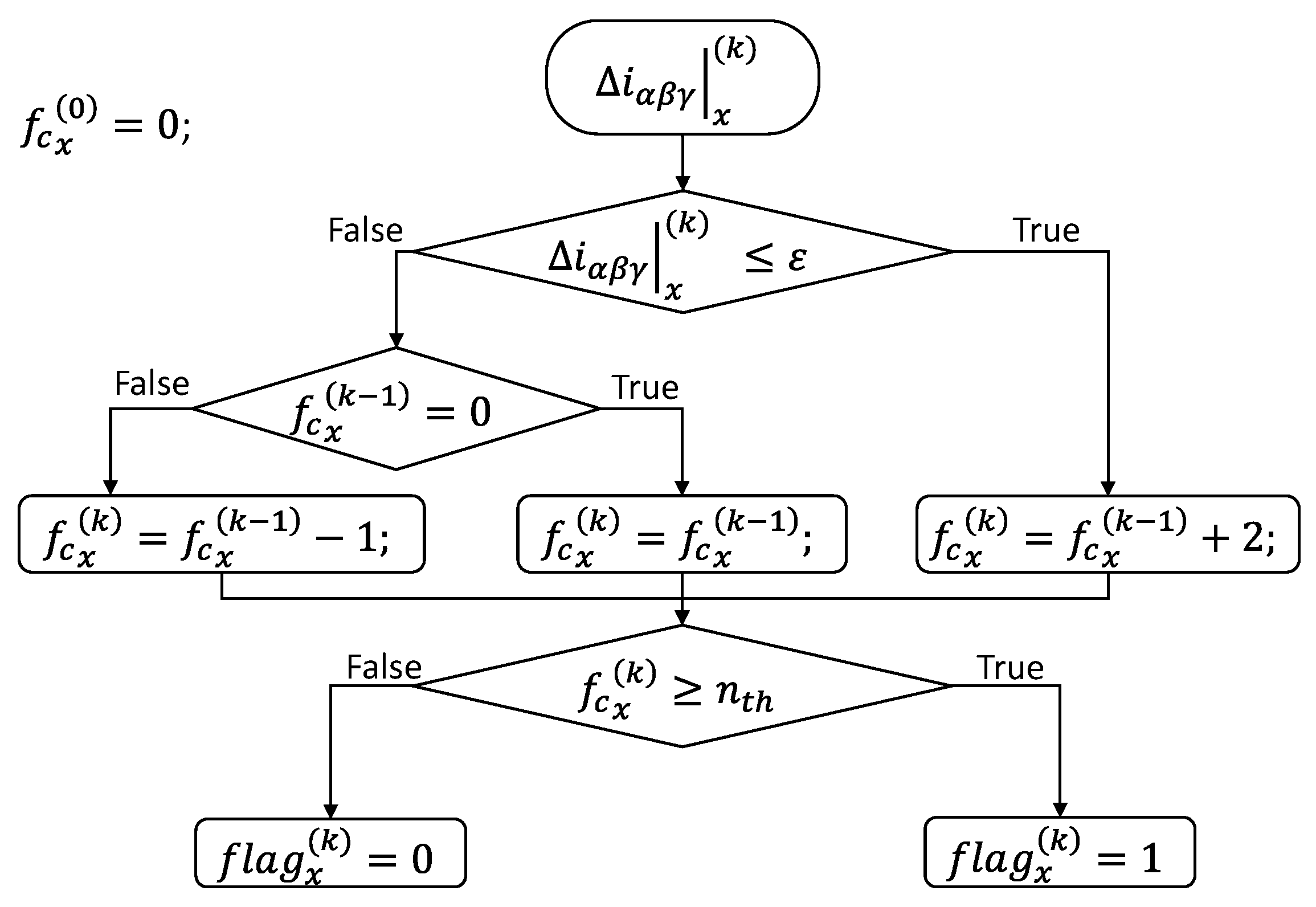
2.4.1. FDI Algorithm

To detect and isolate the open circuit faults, an innovative CS technique is applied, starting from the research documented in [7,20].

In normal conditions, when a PMSM provides torque, the current phasor in the Clarke plane draws a circular trajectory. On the other hand, if an open circuit fault occurs, the motor torque exhibits relevant oscillations and the current phasor in the Clarke plane collapses into a linear segment.

Actually, by applying the Clarke transform, we have that the current component $i_{\gamma }$ represents the current flowing through the central point of the Y connection ($i_n$), and it is zero if the central point is isolated:

$$i_{\gamma }=\frac{1}{\sqrt{3}}\left(i_a+i_b+i_c\right)=\frac{1}{\sqrt{3}}{i}_n=0,$$

(13)

Owing to Equation (13), if an open circuit occurs, the resting two phases are forced to operate in push–pull status. As an example, if the phase a opens, Equation (13) imposes that $i_b=-i_c$, and the current phasor in the Clarke plane draws a linear segment along the β axis. Similarly, if an open circuit affects phase b or phase c, the current phasor will draw linear segments, having slopes $1/\sqrt{3}$ and $-1/\sqrt{3}$, respectively, Figure 5.

The CS technique performs the FDI of open circuit faults by evaluating the current phasor trajectory in the Clarke plane: if it is circular, no faults are detected; if it draws a linear segment, an open circuit is detected and, depending on the orientation of the segment, the fault is also isolated in a specific phase.

The FDI algorithm developed implements two logic sections, executed in series:

 i.

Fault Detection Logic (FDL);

ii.

Fault Isolation Logic (FIL).

The FDL and the FIL are schematically described in the flowchart shown in Figure 6. Though they have the same structure, they are executed on different quantities. In particular, at each $k$-th monitoring sample, if the error $∆i_{\alpha \beta \gamma }{|}_x$ (where x= abc, a, b or c, Equations (14) and (15)) is smaller than a predefined threshold ($\epsilon$), a fault counter $f_{c_x}$ is increased by 2, otherwise it is reduced by 1. When $f_{c_x}$ reaches a predefined maximum value ($n_{th}$), the algorithm outputs a true Boolean fault flag signal $fla{g}_x$. If the algorithm is performed on the quantity $∆i_{\alpha \beta \gamma }{|}_{abc}$ FDL is obtained and the fault flag $fla{g}_{abc}$ represents the detection of a fault. On the other hand, if the algorithm is applied to $∆i_{\alpha \beta \gamma }{|}_a,$ a FIL is obtained and the fault flag $fla{g}_a$ represents the isolation of the fault on phase a (similar considerations can be made for faults on other phases).

$${∆i_{\alpha \beta \gamma }|}_{abc}=\min \left(∆i_{\alpha \beta \gamma }{|}_a, {∆i_{\alpha \beta \gamma }|}_b,{∆i_{\alpha \beta \gamma }|}_c\right),$$

(14)

$$\{\begin{array}{c}{∆i_{\alpha \beta \gamma }|}_a=\left|i_{\alpha }\right|\\ {∆i_{\alpha \beta \gamma }|}_b=\left|i_{\beta }-\frac{i_{\alpha }}{\sqrt{3}}\right|\\ {∆i_{\alpha \beta \gamma }|}_c=\left|i_{\beta }+\frac{i_{\alpha }}{\sqrt{3}}\right|\end{array},$$

(15)

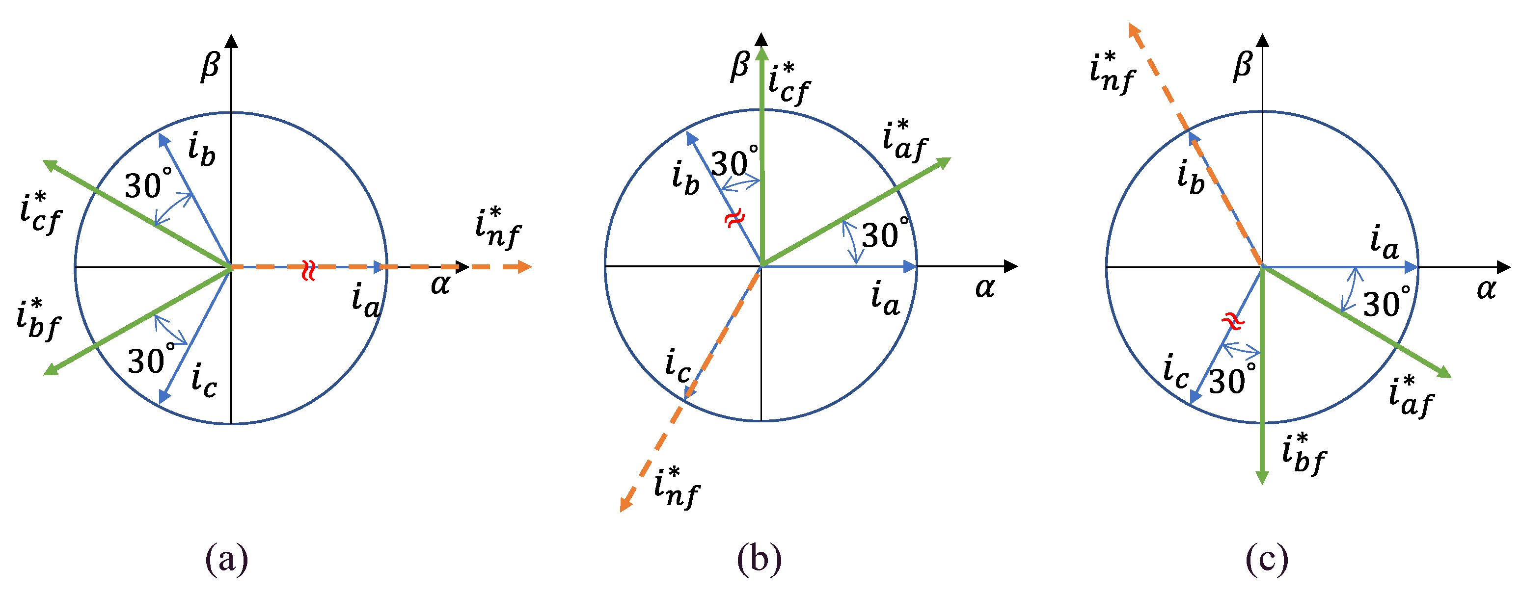
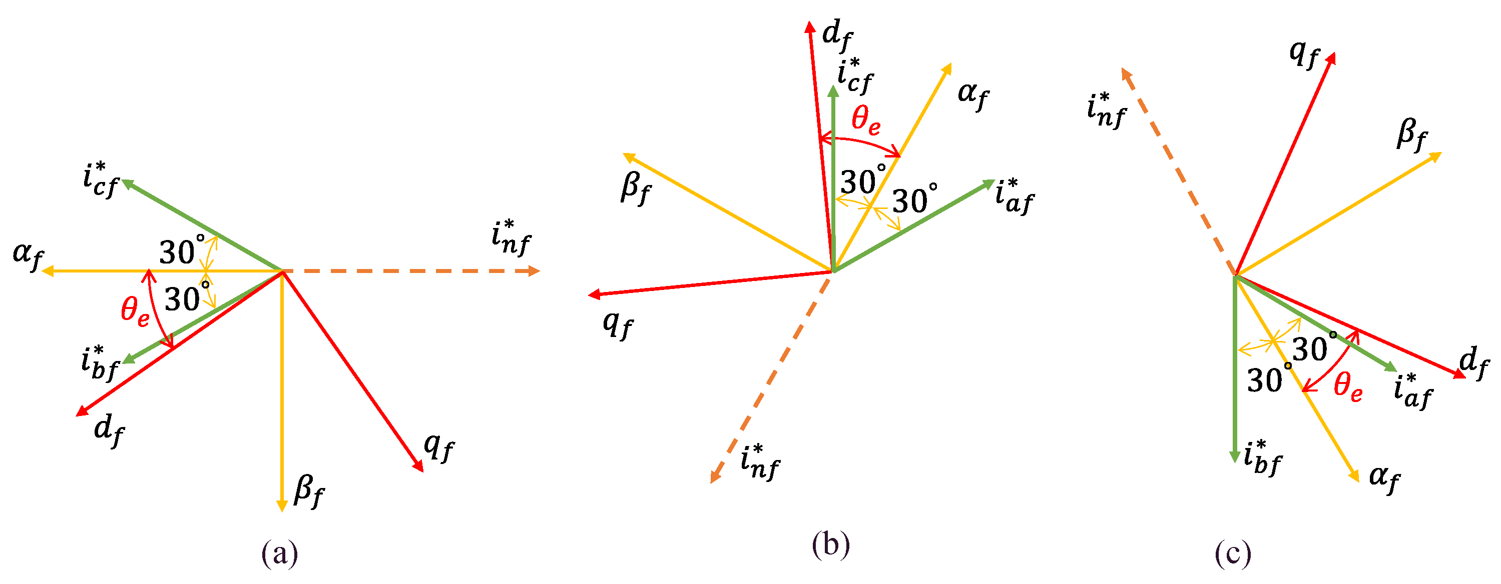
2.4.2. Fault Accommodation Algorithm

When an open circuit fault occurs, the currents in the Park plane contain oscillatory contributions, and the motor output exhibits torque ripples. Hence, to maintain the motor performances after the fault, the control should act in order to restore the current phasor in the Park plane as it was before the fault.

Let us assume that an open circuit is occurred to phase a: if the central point of the Y connection is not isolated, but a neutral point current $i_n$ can be regulated, the zero-sequence current in the Clarke plane, to maintain the same currents on the α and β axes, can be set to

$$i_{\gamma }=-\sqrt{2}{i}_{\alpha },$$

(16)

and consequently the neutral point current is:

$$i_n=-\sqrt{3}{i}_{\gamma }=\sqrt{6}{i}_{\alpha }.$$

(17)

By imposing $i_{\gamma }=-\sqrt{2}{i}_{\alpha }$ in Equations (7) and (8), the post-fault current references for the other two phases $i_{b_f}^{*}$ and $i_{c_f}^{*}$ is by Equation (18):

$$\{\begin{array}{c}{i}_{b_f}^{*}=\sqrt{2}\left(-\frac{\sqrt{3}}{2}{i}_{\alpha }^{*}+\frac{1}{2}{i}_{\beta }^{*}\right)=\sqrt{2}\cos \left(n_d{\theta }_{em}+\frac{7\pi }{6}\right)i_d^{*}-\sqrt{2}\sin \left(n_d{\theta }_{em}+\frac{7\pi }{6}\right)i_q^{*}\\ i_{c_f}^{*}=\sqrt{2}\left(-\frac{\sqrt{3}}{2}{i}_{\alpha }^{*}-\frac{1}{2}{i}_{\beta }^{*}\right)=\sqrt{2}\cos \left(n_d{\theta }_{em}+\frac{5\pi }{6}\right)i_d^{*}-\sqrt{2}\sin \left(n_d{\theta }_{em}+\frac{5\pi }{6}\right)i_q^{*}\end{array},$$

(18)

where $i_{\alpha }^{*}$, $i_{\beta }^{*}$ and $i_d^{*}$, $i_q^{*}$ are the current references before the fault in the Clarke and Park frames, respectively. The neutral point current reference after the fault $i_{n_f}^{*}$ is instead

$$i_{n_f}^{*}=-\sqrt{3}{i}_{\gamma }=\sqrt{6}\cos \left(n_d{\theta }_{em}\right)i_d^{*}-\sqrt{6}\sin \left(n_d{\theta }_{em}\right)i_q^{*}.$$

(19)

By following a similar approach, the current references for the open circuit that occurred to phase b and c can be obtained. A generalized expression is proposed by Equation (20):

$$\{\begin{array}{c}{i}_{xf}^{*}=\sqrt{2}\cos \left[n_d{\theta }_{em}+\frac{2\pi }{3}\left(m+\frac{7}{4}\right)\right]i_d^{*}-\sqrt{2}\sin \left[n_d{\theta }_{em}+\frac{2\pi }{3}\left(m+\frac{7}{4}\right)\right]i_q^{*}\\ i_{yf}^{*}=\sqrt{2}\cos \left[n_d{\theta }_{em}+\frac{2\pi }{3}\left(m+\frac{5}{4}\right)\right]i_d^{*}-\sqrt{2}\sin \left[n_d{\theta }_{em}+\frac{2\pi }{3}\left(m+\frac{5}{4}\right)\right]i_q^{*}\\ i_{wf}^{*}=0\\ i_{nf}^{*}=\sqrt{6}\cos \left(n_d{\theta }_{em}+\frac{2\pi }{3}m\right)i_d^{*}-\sqrt{6}\sin \left(n_d{\theta }_{em}+\frac{2\pi }{3}m\right)i_q^{*}\end{array}$$

(20)

where the subscripts $x$ and $y$ indicate the healthy phases, $w$ the failed phase, while $m$ is an integer number defined by the values given in

Table 2. Reconfiguration parameters.

Failed Phase (w)	x	y	m
a	b	c	0
b	c	a	2
c	a	b	1

.

If one compares the reference currents in normal conditions with the those given by Equation (20), it can be noted that, to maintain the torque performance, the amplitude of the currents in the healthy phases must increase by $\sqrt{3}$ and shift by 60° along the electrical angle (Figure 7), while the amplitude of the neutral point current must be $\sqrt{3}$ times the ones on the healthy state phases, as also reported in [24,28].

It is worth noting that Equation (20) can be conveniently simplified in terms of current phasor in the Park plane, Figure 4b, so that the post-fault current references are:

$$\{\begin{array}{c}{i}_{xf}^{*}=\sqrt{2} I\cos \left[n_d{\theta }_{em}+\phi +\frac{2\pi }{3}\left(m+\frac{7}{4}\right)\right]\\ i_{yf}^{*}=\sqrt{2} I\cos \left[n_d{\theta }_{em}+\phi +\frac{2\pi }{3}\left(m+\frac{5}{4}\right)\right]\\ i_{wf}^{*}=0\\ i_{nf}^{*}=\sqrt{6} I\cos \left(n_d{\theta }_{em}+\phi +\frac{2\pi }{3}m\right)\end{array}.$$

(21)

As outlined in [27], since all the current references in the stator frame are synchronous with the rotor motion, Equation (21), they can be expressed in a rotating frame by applying two transformations (Figure 8):

• From the planar reference ($x_f,y_f, n_f$), to a planar reference frame (${\alpha }_f,{\beta }_f,{\gamma }_f$), in which the ${\alpha }_f$ axis has opposite direction wrt the neutral current axis $n_f$;
• From the planar reference (${\alpha }_f,{\beta }_f,{\gamma }_f$) to a planar rotating frame ($d_f,q_f,z_f$), defined hereafter.

Let us assume that the open circuit is occurred on phase a. With reference to Figure 8a, we have:

$$\left[\begin{array}{c}{i}_{\alpha f}^{*}\\ i_{\beta f}^{*}\\ i_{\gamma f}^{*}\end{array}\right]={\mathit{T}}_{Caf}\left[\begin{array}{c}\begin{array}{c}{i}_{bf}^{*}\\ i_{cf}^{*}\end{array}\\ i_{nf}^{*}\end{array}\right]=\left[\begin{array}{ccc}\frac{\sqrt{3}}{2}& \frac{\sqrt{3}}{2}& -1\\ \frac{1}{2}& -\frac{1}{2}& 0\\ 0& 0& -\frac{1}{\sqrt{3}}\end{array}\right]\left[\begin{array}{c}\begin{array}{c}{i}_{bf}^{*}\\ i_{cf}^{*}\end{array}\\ i_{nf}^{*}\end{array}\right],$$

(22)

while the current phasor in the rotating frame is:

$$\left[\begin{array}{c}{i}_{df}^{*}\\ i_{qf}^{*}\\ i_{zf}^{*}\end{array}\right]={\mathit{T}}_{Paf}\left[\begin{array}{c}{i}_{\alpha f}^{*}\\ i_{\beta f}^{*}\\ i_{\gamma f}^{*}\end{array}\right]=\left[\begin{array}{ccc}{p}_{11}\cos \left(n_d{\theta }_{em}\right)& p_{12}\sin \left(n_d{\theta }_{em}\right)& 0\\ p_{21}\sin \left(n_d{\theta }_{em}\right)& p_{22}\cos \left(n_d{\theta }_{em}\right)& 0\\ 0& 0& 1\end{array}\right]\left[\begin{array}{c}{i}_{\alpha f}^{*}\\ i_{\beta f}^{*}\\ i_{\gamma f}^{*}\end{array}\right],$$

(23)

By substituting Equation (22) into Equation (23), and by recalling Equation (21), we obtain:

$$\left[\begin{array}{c}{i}_{df}^{*}\\ i_{qf}^{*}\\ i_{zf}^{*}\end{array}\right]=\frac{\sqrt{2}}{2}I\left[\begin{array}{c}{P}_1\cos \left(\phi \right)+P_2\cos \left(\phi +2n_d{\theta }_{em}\right)\\ P_3\sin \left(\phi \right)+P_4 sin\left(\phi +2n_d{\theta }_{em}\right)\\ -2\cos \left(\phi +n_d{\theta }_{em}\right)\end{array}\right],$$

(24)

where

$$\begin{array}{cc}{P}_1=\frac{p_{12}}{2}-\left(\frac{3}{2}+\sqrt{3}\right)p_{11},& P_2=-\frac{p_{12}}{2}-\left(\frac{3}{2}+\sqrt{3}\right)p_{11},\\ P_3=\frac{p_{22}}{2}+\left(\frac{3}{2}+\sqrt{3}\right)p_{21},& P_4=\frac{p_{22}}{2}-\left(\frac{3}{2}+\sqrt{3}\right)p_{21}.\end{array}$$

(25)

Thus, to obtain $i_{df}^{*}=i_d^{*}$ and $i_{qf}^{*}=i_q^{*}$, we have:

$$\begin{array}{c}{P}_1=P_3=\sqrt{2},\\ P_4=P_2=0,\end{array}$$

(26)

which leads to

$$p_{11}=-p_{21}=-\frac{\sqrt{2}}{3+2\sqrt{3}}, p_{12}=p_{22}=\sqrt{2}.$$

(27)

As a final result, the transformation matrix from the stator reference frame $\left(b_f,c_f,n_f\right)$ to the rotating frame $\left(d_f,q_f,z_f\right)$ is given by:

$${\mathit{T}}_{paf}{\mathit{T}}_{caf}==[\begin{array}{ccc}{k}_2\sin \left(n_d{\theta }_{em}\right)-k_1\cos \left(n_d{\theta }_{em}\right)& -k_2\sin \left(n_d{\theta }_{em}\right)-k_1\cos \left(n_d{\theta }_{em}\right)& k_3\cos \left(n_d{\theta }_{em}\right)\\ k_1\sin \left(n_d{\theta }_{em}\right)+k_2\cos \left(n_d{\theta }_{em}\right)& k_1\sin \left(n_d{\theta }_{em}\right)-k_2\cos \left(n_d{\theta }_{em}\right)& -k_3\sin \left(n_d{\theta }_{em}\right)\\ 0& 0& -\frac{1}{\sqrt{3}}\end{array}],$$

(28)

where

$$k_1=\frac{\sqrt{6}}{6+4\sqrt{3}}, k_2=\frac{\sqrt{2}}{2}, k_3=\frac{\sqrt{2}}{3+2\sqrt{3}}.$$

(29)

By using a similar approach for the open circuits to the other phases of the motor (see Figure 8b,c), a generalized definition of the transformation matrixes can be obtained:

$$\left[\begin{array}{c}{i}_{df}^{*}\\ i_{qf}^{*}\\ i_{zf}^{*}\end{array}\right]=\left[\begin{array}{ccc}\cos \left(\frac{2\pi }{3}m\right)& -\sin \left(\frac{2\pi }{3}m\right)& 0\\ \sin \left(\frac{2\pi }{3}m\right)& \cos \left(\frac{2\pi }{3}m\right)& 0\\ 0& 0& 1\end{array}\right]{\mathit{T}}_{Paf}{\mathit{T}}_{Caf}\left[\begin{array}{c}\begin{array}{c}{i}_{x_f}^{*}\\ i_{y_f}^{*}\end{array}\\ i_{n_f}^{*}\end{array}\right],$$

(30)

where $m$ is the integer number given in Table 2.

The last step to define the fault accommodation technique requires the calculation of the phase voltage references for the inverter, which are given by the inverse reference frame transformations in the failed conditions.

By assuming again that an open circuit to phase a occurred, the inverse transformation from the rotating frame $\left(d_f,q_f,z_f\right)$ to $(b_f,c_f, n_f)$ is obtained by Equation (31):

$${\left({\mathit{T}}_{paf}{\mathit{T}}_{caf}\right)}^{-1}==[\begin{array}{ccc}\frac{1}{2k_2}\sin \left(n_d{\theta }_{em}\right)-{\frac{1}{2k}}_1\cos \left(n_d{\theta }_{em}\right)& {\frac{1}{2k}}_1\sin \left(n_d{\theta }_{em}\right)+\frac{1}{2k_2}\cos \left(n_d{\theta }_{em}\right)& -1\\ -\frac{1}{2k_2}\sin \left(n_d{\theta }_{em}\right)-{\frac{1}{2k}}_1\cos \left(n_d{\theta }_{em}\right)& {\frac{1}{2k}}_1\sin \left(n_d{\theta }_{em}\right)-\frac{1}{2k_2}\cos \left(n_d{\theta }_{em}\right)& -1\\ 0& 0& -\sqrt{3}\end{array}]$$

(31)

and the voltage references to be imposed in the stator frame are:

$$\left[\begin{array}{c}\begin{array}{c}{V}_{bf}^{*}\\ V_{cf}^{*}\end{array}\\ V_{nf}^{*}\end{array}\right]={\left({\mathit{T}}_{Paf}{\mathit{T}}_{Caf}\right)}^{-1}\left[\begin{array}{c}{V}_{d_f}^{*}\\ V_{q_f}^{*}\\ V_{z_f}^{*}\end{array}\right],$$

(32)

Again, the same as for the direct transformation, a generalized definition of the inverse transformation matrixes can be obtained via Equation (33):

$$\left[\begin{array}{c}\begin{array}{c}{V}_{xf}^{*}\\ V_{yf}^{*}\end{array}\\ V_{nf}^{*}\end{array}\right]={\left({\mathit{T}}_{Paf}{\mathit{T}}_{Caf}\right)}^{-1}\left[\begin{array}{ccc}\cos \left(-\frac{2\pi }{3}m\right)& -\sin \left(-\frac{2\pi }{3}m\right)& 0\\ \sin \left(-\frac{2\pi }{3}m\right)& \cos \left(-\frac{2\pi }{3}m\right)& 0\\ 0& 0& 1\end{array}\right]\left[\begin{array}{c}{V}_{d_f}^{*}\\ V_{q_f}^{*}\\ V_{z_f}^{*}\end{array}\right],$$

(33)

The proposed FTC strategy is schematically reported in Figure 9.

It can be noted that in normal conditions ($fla{g}_x=0$) the conventional transformations are employed (${\mathit{T}}_{\mathit{C}}, {\mathit{T}}_{\mathit{P}}$ and ${\mathit{T}}_{\mathit{P}}^{-\mathbf{1}}, {\mathit{T}}_{\mathit{C}}^{-\mathbf{1}}$) and the neutral point remains isolated ($T_{n1}$ and $T_{n2}$ are open). Once the open circuit fault is detected and isolated by the FDI algorithms in the MON module ($fla{g}_x=1$ with $x=a, b \mathrm{or} c$), the post-fault reference frame transformations are applied (${\mathit{T}}_{{\mathit{C}}_{\mathit{f}}}, {\mathit{T}}_{{\mathit{P}}_{\mathit{f}}}$ and ${\mathit{T}}_{{\mathit{P}}_{\mathit{f}}}^{-\mathbf{1}}, {\mathit{T}}_{{\mathit{C}}_{\mathit{f}}}^{-\mathbf{1}}$) and the voltage references are sent to the four-leg inverter to signal the fourth-leg MOSFET gates ($T_{n1}, T_{n2}$).

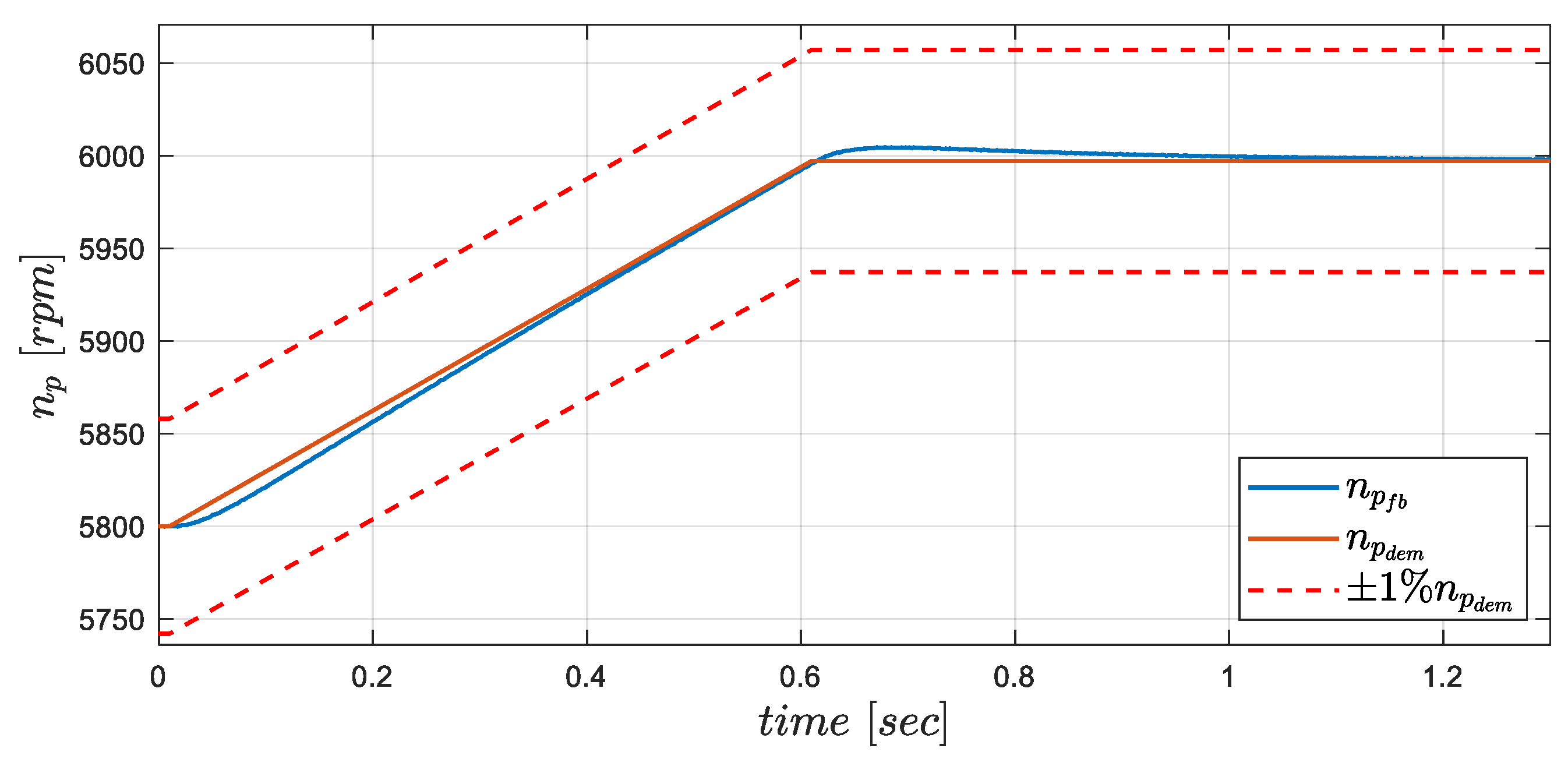
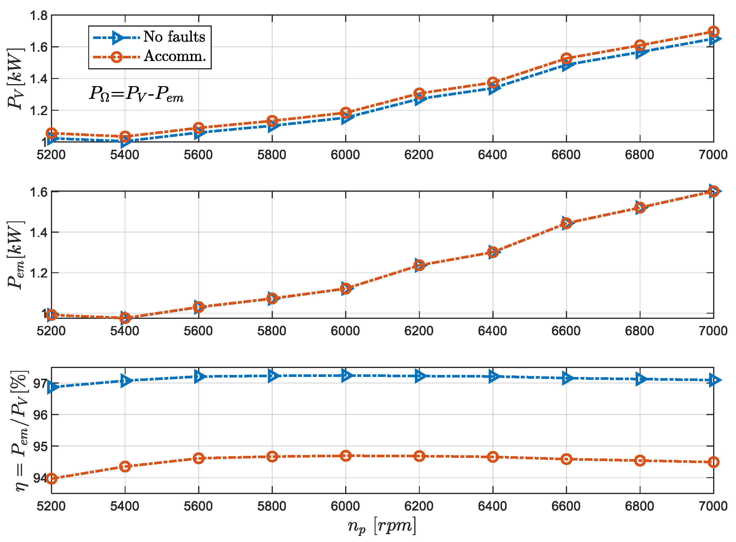
3. Results

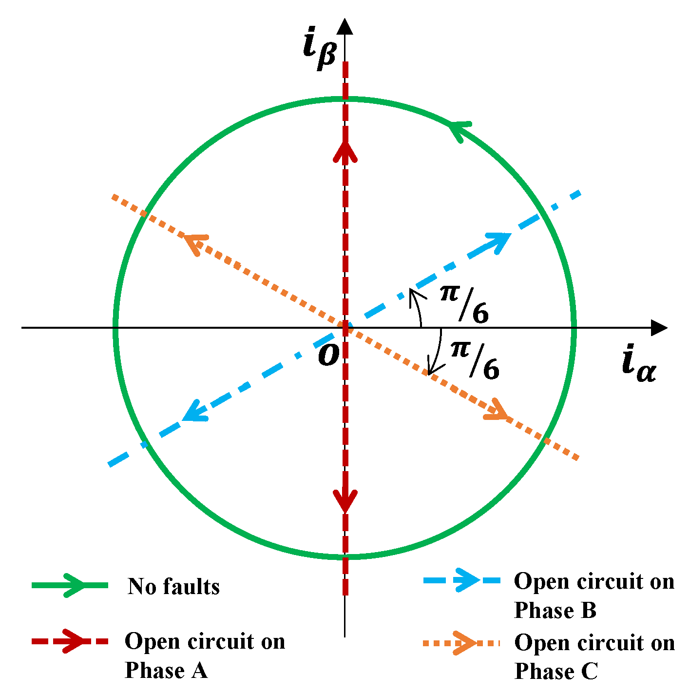
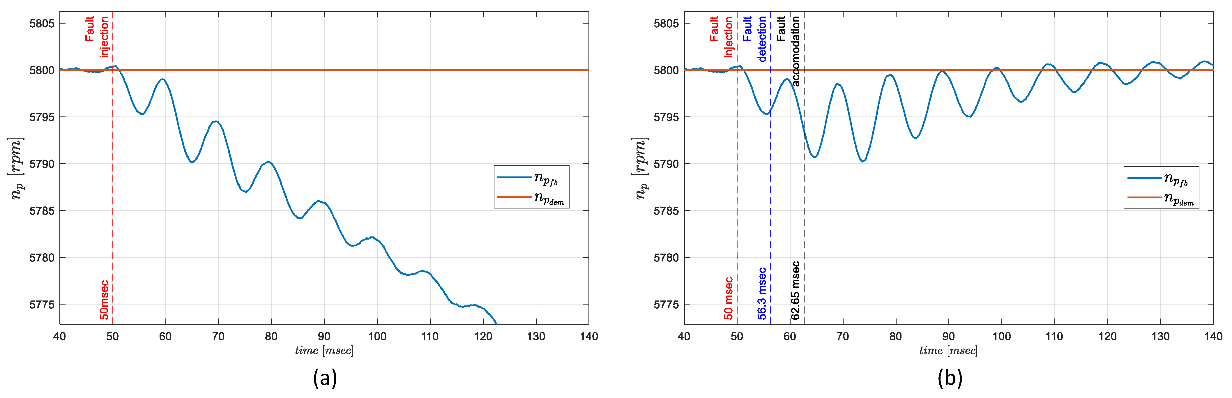
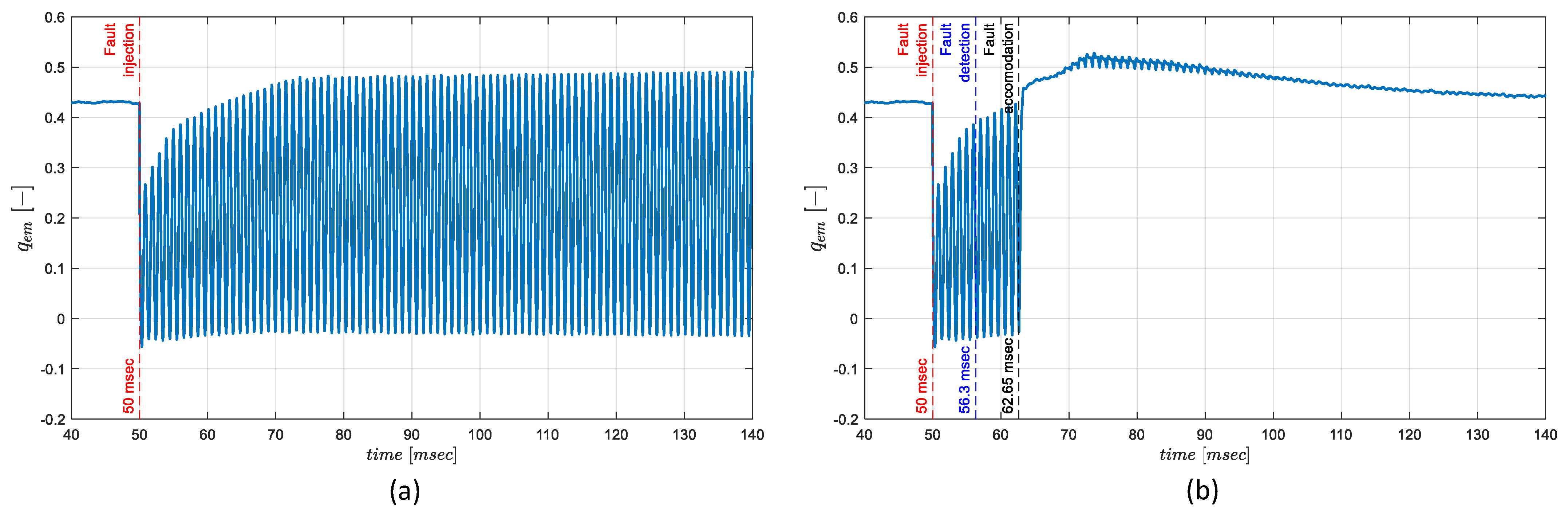
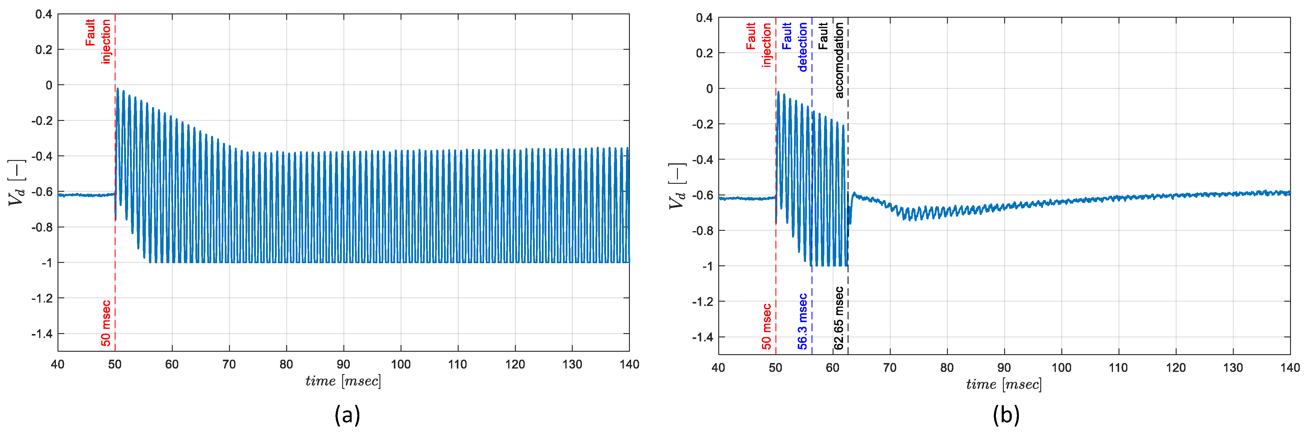
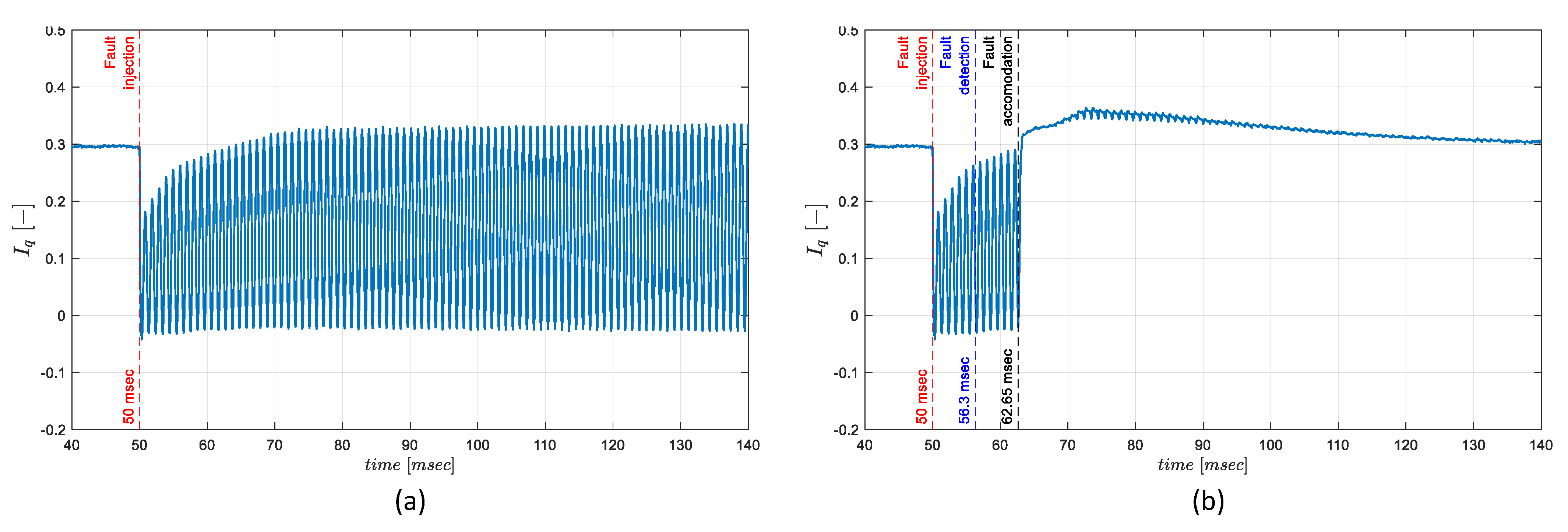
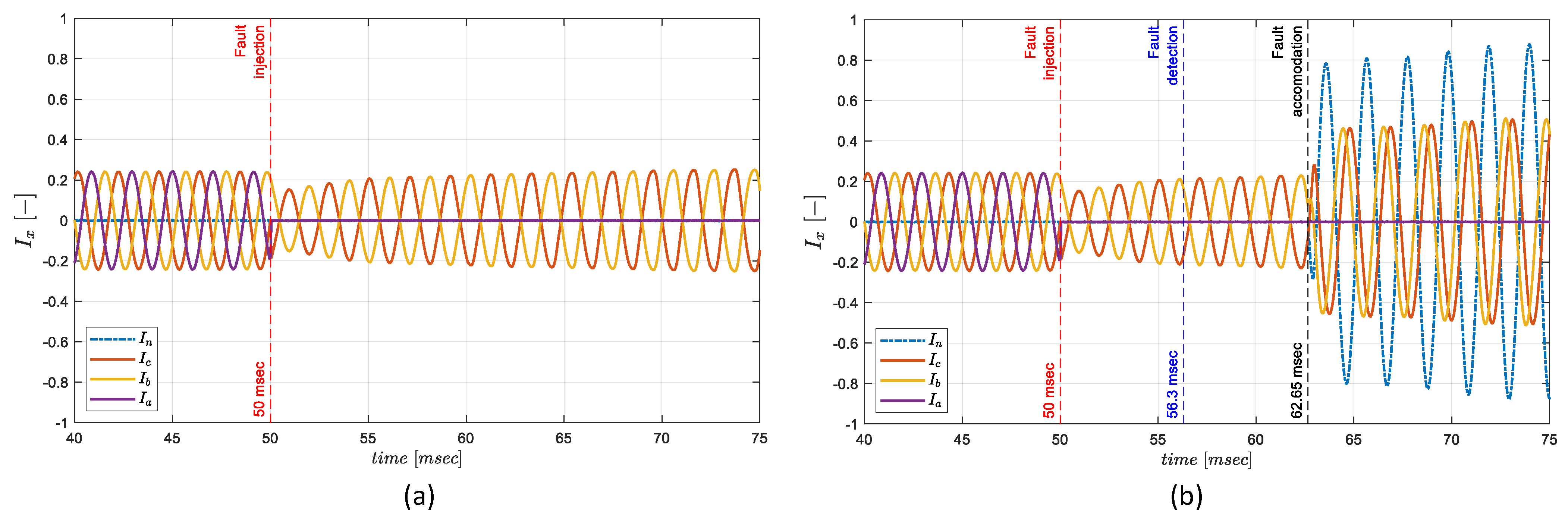
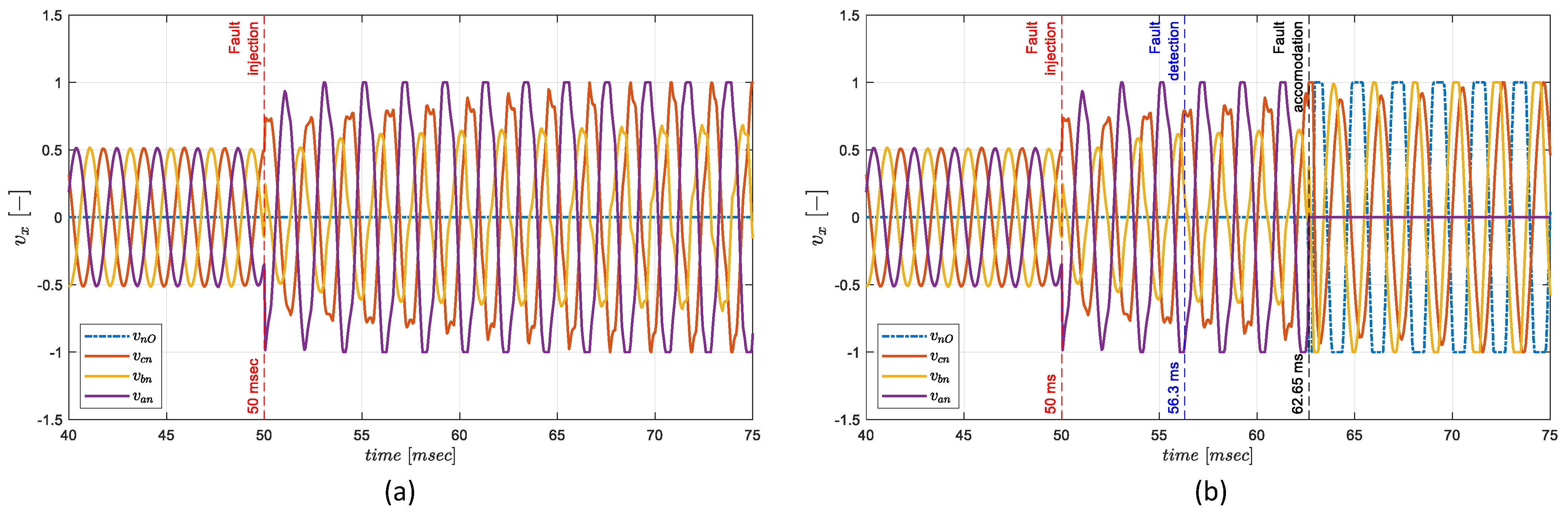
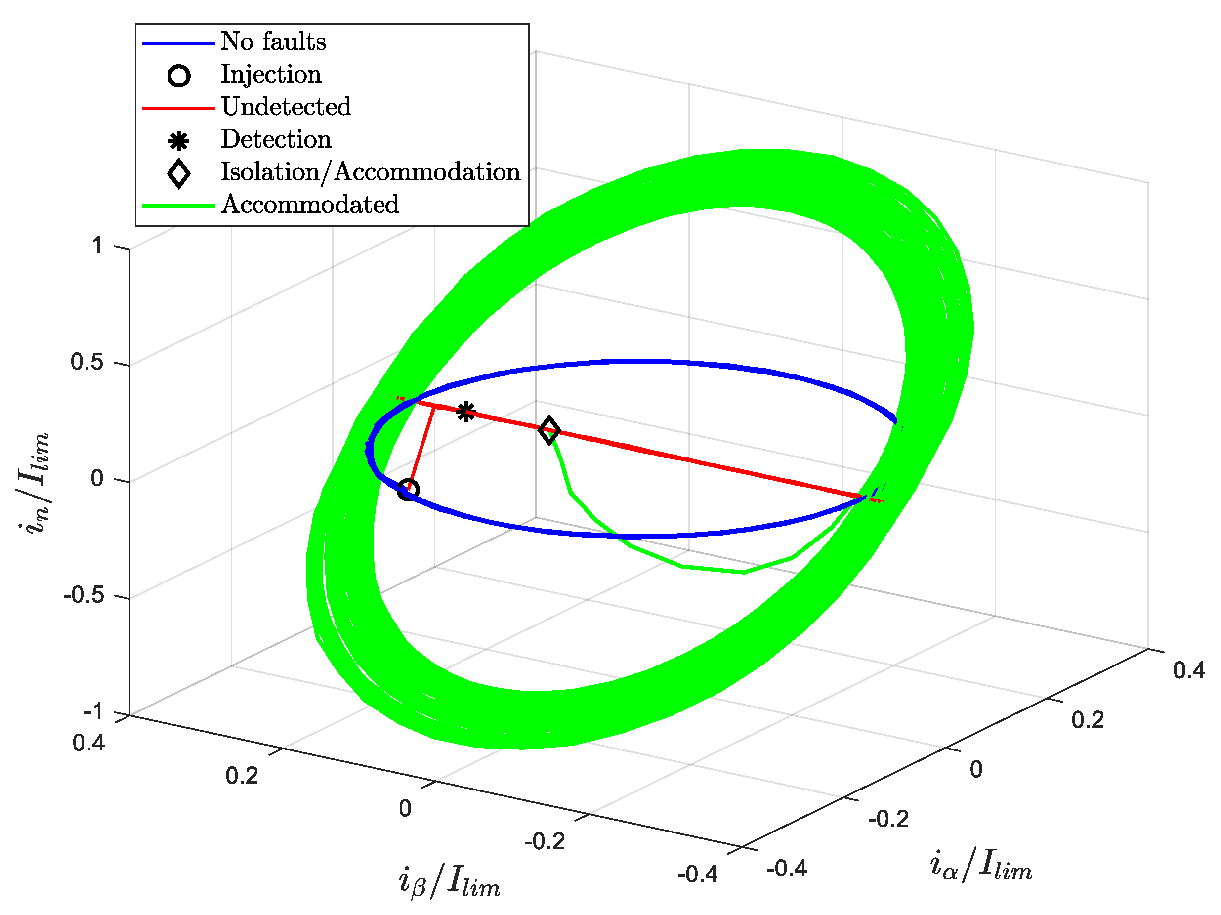
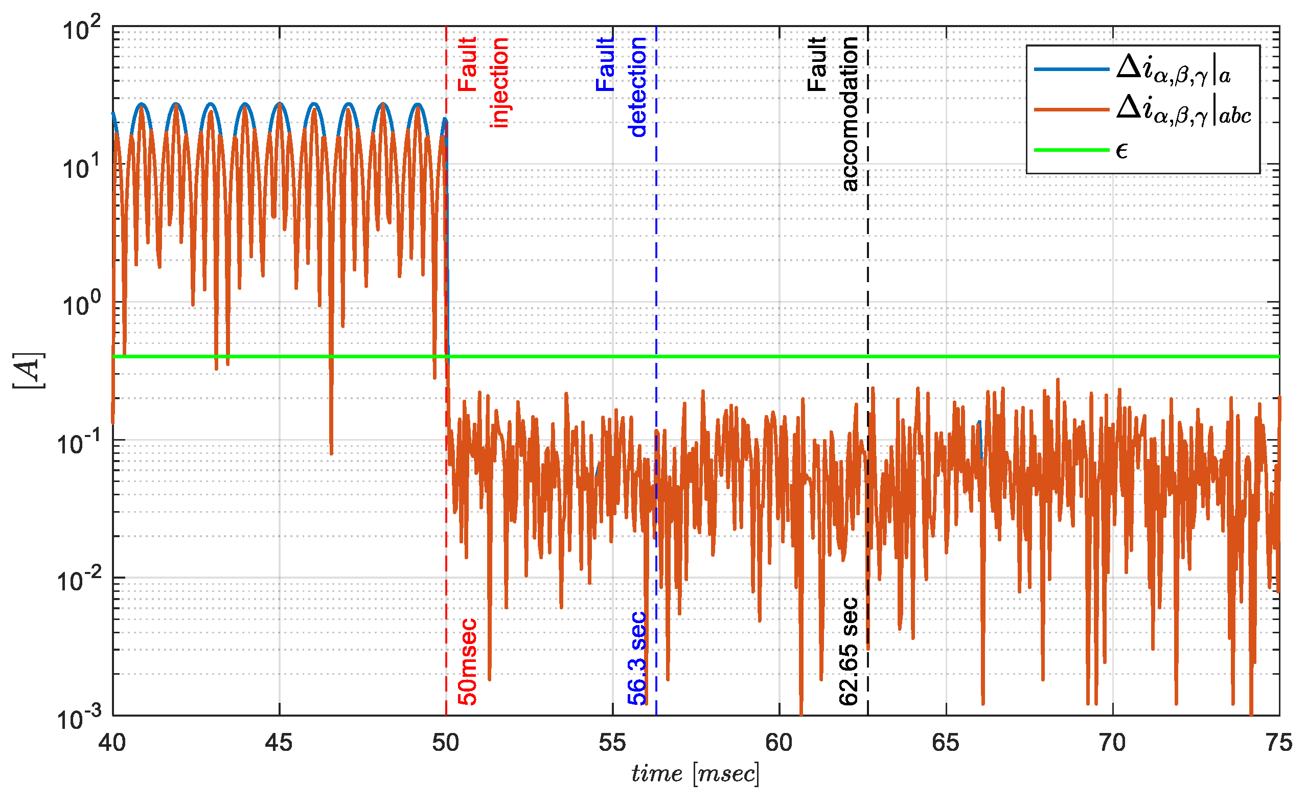
3.1. Failure Transients Characterisation

The effectiveness of the FTC strategy has been tested by using the nonlinear model of the propulsion system. The model has been entirely developed in the MATLAB/Simulink environment, and its numerical solution is obtained via the Runge–Kutta method, with a 10⁻⁵ sec integration step. It is worth noting that the choice of a fixed-step solver is not strictly related to the objectives of this work, in which the model is used for “off-line” simulations testing the FTC, but it has been selected for the next steps of the project, when the FTC system will be implemented in the ECU boards via automatic MATLAB compiler and executed in “real-time”.

Both the closed-loop control and the monitoring functions are executed at 20 kHz sampling rate, and the maximum allowable fault latency has been set to 50 msec. All the simulations started (t = 0 s) with the PMSM in normal conditions, driving the propeller at 5800 rpm with 1.78 Nm torque (related to UAV levelled flight equilibrium at sea level,

Table A3. APC22x10E propeller data.

Definition	Symbol	Value	Unit
Cruise speed	np|cruise	5800	rpm
Cruise torque	Qp|cruise	1.78	Nm
Cruise power	Pp|cruise	1100	W
Climb speed	np|climb	7400	rpm
Climb torque	Qp|climb	4.12	Nm
Climb power	Pp|climb	3238	W

).

Preliminary tests have been carried out to characterise the tracking performance of the closed-loop speed control. In particular, Figure 10 reports the typical response of the speed tracking, when the system is commanded to increase speed to achieve maximum climb rate for the UAV. It can be noted that the system is capable of high dynamic performance in both transient and steady-state phases, with maxima errors lower than 1% of the speed demand.

Successively, the FTC strategy has been assessed by simulating the occurrence of an open circuit fault at t = 50 msec, while the closed-loop control is imposed to maintain the propeller speed value. The system failure transient is thus characterised by applying or not applying the FTC.

The FTC has a great impact on the propeller speed tracking, Figure 11. Once the fault is injected, the propeller speed diverges from the demanded signal if no FTC is used, Figure 11a. On the other hand, the post-fault performance with the FTC is characterised by very small oscillations, which are rapidly extinguished, up to completely recovering the speed reference, Figure 11b. The failure transient characterisation without FTC has been used to quantify the maximum allowable FDI latency, which has been set to 50 msec to limit the propeller speed deviation to less than 0.5% of the reference demand.

Concerning the torque response, the post-fault behaviour without FTC is characterised by high-amplitude high-frequency oscillations, with degradation of the average value with respect to the one before the fault, Figure 12a. This potentially dangerous phenomenon is caused by the abrupt collapse to zero of the current circulating in the failed coil, which implies that the coupling of the magnetic fields generated via FOC technique on the stator system is not synchronous with that of the rotor magnets. The ripple manifests at electrical frequency (about 500 Hz) and potential criticalities can arise if this frequency approaches the structural resonance pulsation of the mechanical train. In the simulation model, the structural resonance occurs at about 100 Hz, but the evaluation is based on preliminary system data. Since the design is ongoing, the point will be addressed via further analyses aiming to verify the interaction between mechanical vibrational modes and post-fault behaviour. On the other hand, the FTC allows for minimising the performance degradation after the fault and the accommodation technique restores the pre-fault torque value within 40 msec, Figure 12b. Similar considerations can be made for direct voltage and quadrature current responses, Figure 13b and Figure 14b.

With particular reference to the direct voltage, due to the high back-electromotive forces, the direct voltage works at about 170 V before the fault, so that, when the fault is injected, it rapidly reaches the saturation value (V_lim = 270 V), Figure 13a.

Due to the open fault on phase a, the remaining phases are forced to a push-pull status until the neutral path is employed, Figure 15. In addition, before the fault accommodation, the phase a voltage increases in amplitude trying to compensate the effects due to the absence of current flow through the phase a, Figure 16.

Another relevant outcome of the simulation study was the identification of the required amplification level for DC–DC supply converter, which has been set to 270 V to let the FTC perform in optimal condition during the accommodation transient.

Figure 17 finally shows the current phasor trajectory in the Clarke space; as expected, when phase a is disconnected the trajectory collapses into a linear segment (red line), while, when the fault is accommodated, the trajectory (green line) expands along the neutral axis and its projection overlaps the circle on the $\alpha ,\beta$ plane, traced before the fault (blue line).

Concerning the power signals, the system with FTC requires an increase of electrical input power (P_V) to balance the growth of copper losses, and this causes a slight reduction of the motor efficiency, Figure 18. From Equation (20), it can be deduced that the copper losses are expected to double in the accommodated status (even with only two active phases), since the current amplitudes in the healthy phases increase by $\sqrt{3}$.

The steady-state performances of the FTC in terms of power and motor efficiency have been finally analysed at different propeller speeds, and then compared with those without faults, Figure 19. As expected, the motor efficiency is always lower, but the trend is essentially constant for speeds ranging $\pm$15% of the cruise speed.

3.2. FDI Parameters Definition

The FDI algorithm developed relies on two parameters, namely the current error threshold ($\epsilon$) and the fault counter threshold (n_th), which have been tuned to optimize the algorithm fault latencies and accuracy (minimum false alarms rate). Consider Figure 20: we reported the currents signals processed for the open-circuit detection ($∆i_{\alpha \beta \gamma }{|}_{abc}$) and isolation ($∆i_{\alpha \beta \gamma }{|}_a$) relative to the simulation presented in the previous section. It can be observed that a combination of high n_th and low ε values is needed to minimise false alarms. On the contrary, low n_th and high ε values are required to increase the detection capability. A good balance has been obtained by imposing $\epsilon =0.4 A$, while, as a first attempt, we used $n_{th}=250$ to essentially eliminate false alarms.

4. Discussion

A comparative analysis with relevant works from the literature was carried out in terms of FDI performances. The results of this activity are proposed in

Table 3. FDI performances of the proposed algorithm compared with literature results.

Method	Latency [ms]	Monitor Frequency [kHz]	Electrical Frequency [Hz]	Monitor Samples Per Electrical Period
ZSVC [19]	$40$	$20$	$12$	1666
CSD [21]	$20$	$20$	$45$	445
AAV [22]	$6.6$	$40$	$100$	400
CSnD	$13$	$20$	$480$	42

ZSVC: Zero-Sequence Voltage Component; CSD: Current Signature Derivative; AAV: Absolute Average Voltage; CSnD: Current Signature no-Derivative.

. The most relevant outcome is that the proposed algorithm (CSnD) is capable of very small latencies with the lowest number of monitoring samples per electrical period. Actually, it is worth noting that the reference application is characterised by a motor speed that is much higher than the ones used in literature reports.

Compared with the CSD algorithm [21], the developed one is similar, but it does not use derivative operators, which raise concerns in terms of noise contents. The detection latency with CSD is slightly worse, but (above all) it is obtained with about ten times the monitoring samples with respect to the proposed algorithm. Concerning the AAV algorithm [22], its latency is lower, but it is obtained with ten times the monitoring samples per electrical period. Finally, the proposed CSnD technique performs better than the ZSVC method [19] in terms of both latency and utilized monitoring samples.

Concerning the fault accommodation issues, if compared with other strategies applied on four-leg inverters (

Table 4. Fault-tolerant control performances compared with literature results.

Control Strategy	Control Laws Robustness	Torque Ripple	Average Torque Degradation
SCHC [25,26]	Average	Average	Average
RCHC [26]	Average	High	High
RCFFC [24,25,26]	Low	Average	Negligible
RCFTC	High	Low	Negligible

SCHC: Stator Currents Hysteresis Control; RCHC: Rotor Currents Hysteresis Control; RCFFC: Rotor Currents Feed-Forward Control; RCFTC: Rotor Currents Frame Transformation Control.

), the proposed technique permits better torque performances (low torque ripple and no degradation of average value with respect to the ones before the fault) and good robustness, since neither control reconfiguration nor feedforward compensation are introduced to counteract the faulty behaviour. Though the SCHC strategy (applying a hysteresis control on $a,b,c,n$ currents [25,26]) shows higher robustness compared with RCFFC, it suffers from the variable switching frequency, which reduces the control accuracy (noticeable torque ripple and torque degradation are observed). Similarly, the RCHC strategy (applying a hysteresis control on $d,q,z$ currents [26]) is characterized by low robustness and poor post-fault performances [26].

Considering this discussion, the most relevant findings of the work can be summarised as follows:

• The CSnD FDI algorithm provides the smallest ratio between detection latency and monitoring samples per electrical period;
• The fault accommodation technique provides very satisfactory torque performances without implementing control laws reconfiguration or feedforward compensation in the closed-loop architecture.

It is worth mentioning that, though the FTC presented has been applied to open-circuit faults only, it can be extended to all PMSM electrical faults. In particular, in the case of MOSFET faults, the phasor trajectory in the Clarke plane draws a half-circle closed by a linear segment [21], and the segment slope can be employed (similar to what is done in this work) to identify the faulty leg, while the missing half-cycle of the phasor trajectory can be used to locate the faulty switch. In case of short-circuits, the phasor trajectory in the Clarke plane instead deforms into an elliptical shape, with an orientation that depends on the shorted phase. For this fault mode, the proposed strategy cannot be directly applied, and it should be reformulated.

In the next steps of the research, the validation of the FTC strategy is foreseen. This is planned to be carried out by:

• Experimental testing, aiming to

  ○

  validate the model predictions in case of faults (by excluding the FTC),

  ○

  characterise the fault accommodation latencies (by “forcing” its activation without faults).

• Enhanced simulation analysis, including the detailed modelling of the MOSFET power bridge, to refine the predictions of failure transients.

5. Conclusions

A fault-tolerant control strategy for a high-speed PMSM with four-leg inverter employed for UAV propulsion is developed and characterised in terms of fault-detection/isolation latencies and accommodation capabilities. The FDI and fault accommodation performances of the FTC are assessed via simulation, by using a nonlinear model of the electrical propulsion system, by injecting open-circuit phase faults. The proposed strategy, based on an innovative current signature technique, allows for detecting the fault within six electrical cycles, by executing 40 monitoring tasks per cycle. In addition, the accommodation technique minimises the failure transient and allows for complete recovery of the system performance with negligible efficiency reduction. Future developments of the research will focus on the extension of the method to short-circuit faults and MOSFETs faults.

References

- “Unmanned Aerial Vehicle (UAV) Market by Point of Sale, Systems, Platform (Civil & Commercial, and Defense & Governement), Function, End Use, Application, Type, Mode of Operation, MTOW, Range, and Region—Global Forecast to 2026”; RESEARCH AND MARKETS; 16 December 2020; Available online: https://www.researchandmarkets.com/reports/5350868/unmanned-aerial-vehicle-uav-market-by-point-of#src-pos-1 (accessed on 7 September 2021).
- Suti, A.; Di Rito, G.; Galatolo, R. Climbing performance enhancement of small fixed-wing UAVs via hybrid electric propulsion. In Proceedings of the 2021 IEEE Workshop on Electrical Machines Design, Control and Diagnosis (WEMDCD), Modena, Italy, 8–9 April 2021. [Google Scholar] [CrossRef]
- Mamen, A.; Supatti, U. A Survey of Hybrid Energy Storage Systems Applied for Intermittent Renewable Energy Systems. In Proceedings of the 14th International Conference on Electrical Engineering/Electronics, Computer, Telecommunications and Information Technology (ECTI-CON), Phuket, Thailand, 27–30 June 2017. [Google Scholar] [CrossRef]
- Nandi, S.; Toliyat, H.A.; Li, X. Condition Monitoring and Fault Diagnosis of Electrical Motors—A Review. IEEE Trans. Energy Convers. 2005, 20, 719–729. [Google Scholar] [CrossRef]
- Kontarček, A.; Bajec, P.; Nemec, M.; Ambrožič, V.; Nedeljković, D. Cost-Effective Three-Phase PMSM Drive Tolerant to Open-Phase Fault. IEEE Trans. Ind. Electron. 2015, 62, 6708–6718. [Google Scholar] [CrossRef]
- Cao, W.; Mecrow, B.C.; Atkinson, G.J.; Bennett, J.W.; Atkinson, D.J. Overview of Electric Motor Technologies Used for More Electric Aircraft (MEA). IEEE Trans. Ind. Electron. 2012, 59, 3523–3531. [Google Scholar] [CrossRef]
- Khalaief, A.; Boussank, M.; Gossa, M. Open phase faults detection in PMSM drives based on current signature analysis. In Proceedings of the XIX International Conference on Electrical Machines (ICEM 2010), Roma, Italy, 6–8 September 2010. [Google Scholar] [CrossRef]
- Li, W.; Tang, H.; Luo, S.; Yan, X.; Wu, Z. Comparative analysis of the operating performance, magnetic field, and temperature rise of the three-phase permanent magnet synchronous motor with or without fault-tolerant control under single-phase open-circuit fault. IET Electr. Power Appl. 2021, 15, 861–872. [Google Scholar] [CrossRef]
- Ryu, H.-M.; Kim, J.-W.; Sul, S.-K. Synchronous-frame current control of multiphase synchronous motor under asymmetric fault condition due to open phases. IEEE Trans. Ind. Appl. 2006, 42, 1062–1070. [Google Scholar] [CrossRef]
- Liu, G.; Lin, Z.; Zhao, W.; Chen, Q.; Xu, G. Third Harmonic Current Injection in Fault-Tolerant Five-Phase Permanent-Magnet Motor Drive. IEEE Trans. Power Electron. 2018, 33, 6970–6979. [Google Scholar] [CrossRef]
- Bennet, J.W.; Mecrow, B.C.; Atkinson, D.J.; Atkinson, G.J. Safety-critical design of electromechanical actuation systems in commercial aircraft. IET Electr. Power Appl. 2009, 5, 37–47. [Google Scholar] [CrossRef]
- Mazzoleni, M.; Di Rito, G.; Previdi, F. Fault Diagnosis and Condition Monitoring Approaches. In Electro-Mechanical Actuators for the More Electric Aircraft; Advances in Industrial Control; Springer: Cham, Switzerland, 2021. [Google Scholar] [CrossRef]
- de Rossiter Correa, M.B.; Jacobina, C.B.; Da Silva, E.C.; Lima, A.N. An Induction Motor Drive System with Improved Fault Tolerance. IEEE Trans. Ind. Appl. 2001, 37, 873–879. [Google Scholar] [CrossRef]
- Ribeiro, R.L.A.; Jacobina, C.B.; Lima, A.M.N.; da Silva, E.R.C. A strategy for improving reliability of motor drive systems using a four-leg three-phase converter. In Proceedings of the APEC 2001, Sixteenth Annual IEEE Applied Power Electronics Conference and Exposition (Cat. No. 01CH37181), Anaheim, CA, USA, 4–8 March 2001. [Google Scholar] [CrossRef]
- Kontarček, A.; Bajec, P.; Nemec, M.; Ambrožič, V. Single open-phase fault detection in permanent magnet synchronous machine through current prediction. In Proceedings of the IECON 2013—39th Annual Conference of the IEEE Industrial Electronics Society, Vienna, Austria, 10–13 November 2013. [Google Scholar] [CrossRef]
- Saleh, A.; Sayed, N.; Abdel, G.A.; Eskander, M.N. Fault-Tolerant Control of Permanent Magnet Synchronous Motor Drive under Open-Phase Fault. Adv. Sci. Technol. Eng. Syst. J. 2020, 5, 455–463. [Google Scholar] [CrossRef]
- Park, B.-G.; Jang, J.-S.; Kim, T.-S.; Hyun, D.-S. EKF-based fault diagnosis for open-phase faults of PMSM drives. In Proceedings of the 2009 IEEE 6th International Power Electronics and Motion Control Conference, Wuhan, China, 17–20 May 2009. [Google Scholar] [CrossRef]
- Gajanayake, C.J.; Bhangu, B.; Nadarajan, S.; Jayasinghe, G. Fault tolerant control method to improve the torque and speed response in PMSM drive with winding faults. In Proceedings of the 2011 IEEE Ninth International Conference on Power Electronics and Drive Systems, Singapore, 5–8 December 2011. [Google Scholar] [CrossRef]
- Jun, H.; Jianzhong, Z.; Ming, C.; Shichuan, D. Detection and Discrimination of Open-Phase Fault in Permanent Magnet Synchronous Motor Drive System. IEEE Trans. Power Electron. 2016, 31, 4697–4709. [Google Scholar] [CrossRef]
- Huang, J.; Zhang, Z.; Jiang, W. Fault-tolerant control of open-circuit fault for permanent magnet starter/generator. In Proceedings of the 21st International Conference on Electrical Machines and Systems (ICEMS), Jeju, Korea, 7–10 October 2018. [Google Scholar] [CrossRef]
- Peuget, R.; Courtine, S.; Rognon, J.-P. Fault detection and isolation on a PWM inverter by knowledge-based model. IEEE Trans. Ind. Appl. 2016, 34, 1318–1326. [Google Scholar] [CrossRef]
- Estima, J.O.; Cardoso, A.J.M. A New Approach for Real-Time Multiple Open-Circuit Fault Diagnosis in Voltage-Source Inverters. IEEE Trans. Ind. Appl. 2011, 47, 2487–2494. [Google Scholar] [CrossRef]
- Estima, J.O.; Freire, N.M.A.; Cardoso, A.J.M. Recent advances in fault diagnosis by Park’s vector approach. In Proceedings of the 2013 IEEE Workshop on Electrical Machines Design, Control and Diagnosis (WEMDCD), Paris, France, 11–12 March 2013. [Google Scholar] [CrossRef]
- Bolognani, S.; Zordan, M.; Zigliotto, M. Experimental fault-tolerant control of a PMSM drive. IEEE Trans. Ind. Electron. 2000, 47, 1134–1141. [Google Scholar] [CrossRef]
- Bianchi, N.; Bolognani, S.; Zigliotto, M.; Zordan, M. Innovative remedial strategies for inverter faults in IPM synchronous motor drives. IEEE Trans. Energy Convers. 2003, 18, 306–314. [Google Scholar] [CrossRef]
- Meinguet, F.; Gyselinck, J. Control strategies and reconfiguration of four-leg inverter PMSM drives in case of single-phase open-circuit faults. In Proceedings of the 2009 IEEE International Electric Machines and Drives Conference, Miami, FL, USA, 3–6 May 2009. [Google Scholar] [CrossRef]
- Xinxiu, Z.; Jun, S.; Haitao, L.; Xinda, S. High Performance Three-Phase PMSM Open-Phase Fault-Tolerant Method Based on Reference Frame Transformation. IEEE Trans. Ind. Electron. 2019, 66, 7571–7580. [Google Scholar] [CrossRef]
- Xinxiu, Z.; Jun, S.; Haitao, L.; Ming, L.; Fanquan, Z. PMSM Open-Phase Fault-Tolerant Control Strategy Based on Four-Leg Inverter. IEEE Trans. Power Electron. 2020, 35, 2799–2808. [Google Scholar] [CrossRef]
- APC Propellers TECHNICAL INFO. Available online: https://www.apcprop.com/technical-information/performance-data/ (accessed on 2 May 2021).
- Seung-ki, S. Reference Frame Transformation and Transient State Analysis of Three-Phase AC Machines. In Control of Electric Machine Drive Systems, 1st ed.; Wiley-IEEE Press: Hoboken, NJ, USA, 2010. [Google Scholar] [CrossRef]
- Caruso, M.; Di Tommaso, A.O.; Miceli, R.; Nevolos, C.; Spataro, C.; Trapanese, M. Maximum Torque per Ampere Control Strategy for Low-Saliency Ratio IPMSMs. Int. J. Renew. Energy Res. IJRER 2019, 9, 374–383. Available online: https://www.ijrer.org/ijrer/index.php/ijrer/article/view/9057 (accessed on 7 September 2021).