
An Extended Model for Ripple Analysis of 2–4 Phase Resonant Electrostatic Induction Motors
by
 , , and
Fernando Carneiro
1,* ,
,
Guangwei Zhang
2 ,
,
Masahiko Osada
1,3,
Shunsuke Yoshimoto
2 and
Akio Yamamoto
2,* 1
Department of Precision Engineering, Graduate School of Engineering, The University of Tokyo, Tokyo 113-8656, Japan
2
Department of Human and Engineered Environmental Studies, Graduate School of Frontier Sciences, The University of Tokyo, Chiba 277-8563, Japan
3
Frontier Robotics, Honda R&D Co., Ltd., Saitama 351-0188, Japan
*
Authors to whom correspondence should be addressed.
Actuators 2021, 10(11), 291; https://0-doi-org.brum.beds.ac.uk/10.3390/act10110291
Submission received: 29 July 2021
/
Revised: 15 October 2021
/
Accepted: 26 October 2021
/
Published: 29 October 2021
(This article belongs to the Section Precision Actuators)
Abstract
:Electrostatic motors are promising forms of actuation for future robotic devices. The study of their different implementations should accelerate their adoption. Current models for resonant electrostatic induction motors were found not to be able to properly describe their behavior, namely, with regard to changes with position. This paper reports a new analytical model for these motors, aiming to address this issue. The model is based on identification of all capacitance harmonics, through a simplified method. Using these, equations for different motor parameters, notably, thrust force, were obtained and compared to previous literature. The new equations model position dependent properties, such as force ripple. The outputs of this model were validated through experimentation with a prototype, with the results confirming the new model better describes motor behavior. An analysis into how to decrease this ripple was also discussed and tested. We concluded that the use of a higher number of harmonics resulted in a much more accurate model, capable of adequately characterizing motor outputs with changes in position.
1. Introduction
Traditionally, an actuated mechanism comprises a rigid structure and an actuator. For small-scale robots, this actuator is most times a conventional electromagnetic motor. However, there is an increasing demand for alternative forms of actuation, driven partly by attempts to replicate biological shapes and movements, in the pursuit of higher performance, lower weight or capabilities that go beyond simple manipulation or movement [1]. There is an abundance of ongoing research on this topic, with recent results including robots capable of swimming [2], jumping [3,4], wall climbing [5,6] and flapping-wing flight [7] in a biologically-inspired manner, thanks to the application of unconventional forms of actuation. A subset of these is the field of soft robotics, which focuses on the development of robots with soft structures, not only for biomimetic purposes [8], but also as a form of enhancing safety when interacting with human beings [9]. These soft or compliant robots can be materialized in a number of ways using fluid [10,11,12,13], thermal [14,15] or electrostatic [6,16] actuation, on which the present paper will focus.
The electrostatic force is the fundamental principle for several very distinct forms of actuation currently under study. These include direct interaction with particulate material [17], compression of elastomeric substrates [16,18] and by exploiting corona discharge [19]. There are also other, more direct, applications such as by using charged metal pegs [20] and thin films [21,22,23]. The electrostatic actuators approached in this paper are those realized using thin films. These motors are materialized as thin polymeric films with embedded copper electrodes. Movement is achieved by the electrostatic interaction between electrodes in different sets of films. These motors have been shown to produce considerable force [24] and potential for integration in robotic actuation [25]. Their high performance, coupled with manufacturing using flexible substrates and inherent low weight, makes them strong candidates for actuating robotic mechanisms in the future.
These motors can be classified into two main categories: dual excitation [22] and induction [23,26] type motors. The dual excitation type motors operate synchronously, and require all motor films (stator and slider/rotor) to be directly connected to a multi-phase AC voltage power source. The wiring to the moving parts may cause disturbances in the motion control or even lead to faster wear of the wires/brushes. In the case of the induction motor, only the stator needs to be directly powered. For this motor, voltage is transmitted to the slider elements through induction. Initial implementations of this kind of motor employed a fully passive slider, with no electrodes, resulting in lower thrust force [23]. However, more recent progress has resulted in a hybrid motor which uses the same electrode structure of the dual excitation motor for the induction version [26]. To generate high voltages on the slider elements, and achieve thrust force comparable to the dual excitation type, this motor uses LC resonance. By connecting inductors between the electrodes of the slider films, they form LC circuits with the motor. This boosts the slider voltage when driven at its resonant frequency, and enables a wireless slider, as the inductors can be attached to or incorporated into the films.
Initial implementations of the LC resonant electrostatic film motors used a 3-phase topology, leading to capacitance imbalance [27]. More recently, a 2–4 phase architecture has been explored [28]. This approach uses four phases on the stator and two on the slider, which enables the use of a single inductor, eliminating the effects of capacitance imbalance. This also simplifies driving, as the stator is driven with 4-phase voltage, which can be generated using only two transformers.
Although this motor has been modeled in the past [28], the model has been found to not adequately describe the behaviour of the current prototype [29]. Specifically, the current motor exhibits force ripple, possibly due to different electrodes geometry from the previous version. Similar force ripple was also seen and analyzed for the dual-excitation motor. However, the behavior of the force ripple in the induction motor seems much more complicated.
Therefore, to understand the characteristics of the force ripple in the induction motor, this paper proposes a new motor model such that it can evaluate the force ripple. In the previous work on the dual excitation type, it was found that harmonics in the capacitance variations create force ripple. However, the harmonics were not considered in the previous studies on LC-resonance type. This work evaluates the capacitance variations in the motor and proposes a model including the harmonics. Using the model, the paper provides equations describing induced slider voltages and thrust force, to reveal how motor parameters affect the force ripple.
In this paper, following this introduction, an explanation of the motor structure and working principle are provided. Then, a new motor model is described in Section 3, which is analyzed in comparison with the previous model in Section 4. The model behavior is validated using a prototype LC-resonance type motor in Section 5. Section 6 concludes.
2. Electrostatic Induction Motor with 2–4 Phase Electrodes
2.1. Structure and Operation
Like other electrostatic film motors, the LC-resonance motor can be realized both in linear and rotary fashions. As the models are the same for both linear and rotary, this work adopts linear one without losing generality.
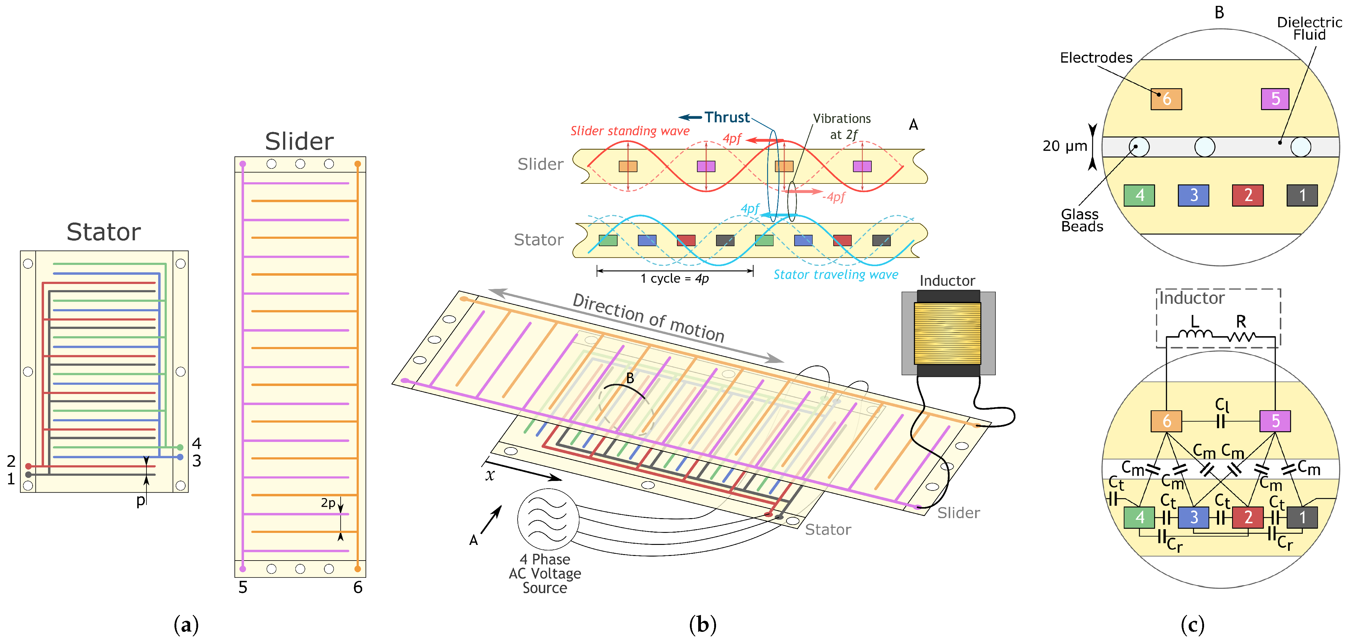
The motor reported in this paper consists of two polymeric films with evenly-spaced parallel copper electrodes, which are often fabricated using flexible printed circuit (FPC) technologies. Within each film, the electrodes are connected in sets, which we designate as phases. The slider film contains two sets of electrodes, or two phases, while the stator comprises four phases, thus the 2–4 phase designation. For operation, glass beads are scattered between the stator and the slider films for reducing friction. They are also immersed in dielectric fluid, to prevent discharge due to the high voltages used. An illustration of this structure can be seen in Figure 1. Although the motor can be materialized with different numbers of films [30], this paper focuses on the version with one stator film and one slider film, as it is the most elementary example.
The electrode pitch is different between the slider and the stator, due to the different numbers of phases. The slider has twice as large pitch as the stator, which results in the same length of the electrode cycles. In this paper, the pitch for the stator electrodes is defined as p, while that for the slider electrodes is 2p.
The force produced by the motor is overall proportional to the product of both stator and slider voltages, so these should be as high as the material allows, typically reaching values of ~1500 V0-pk. For the stator electrodes, those high voltages are directly fed from voltage sources through wires. On the other hand, the voltages to the slider are provided by electrostatic induction and amplified by LC resonance. Taking advantage of the motor’s intrinsic capacitance, an inductor is connected between the slider’s two phases to enable this amplification. The added inductance and the driving frequency must be selected concertedly to enable the desired voltage amplification.
The 4-phase AC voltages, applied to the 4-phase electrodes on the stator, spatially create a traveling voltage wave on the stator surface. This wave travels at a speed of , where f is the applied frequency. On the slider electrodes, in a stationary state, a high voltage with the same frequency of the stator voltage is induced, whose voltage phase depends on the position of the slider electrode. As the two electrode phases are shifted, in terms of their positions, by a half cycle, the voltages induced on the two phases will have 180 degrees phase shift. This will spatially create a standing voltage wave on the slider. The standing wave can be decomposed into two voltage waves that travel in opposite directions at the same absolute speed, . One of the decomposed waves travels in the same direction as the stator wave. This wave interacts with the stator wave to create tangential electrostatic force, whose magnitude depends on the spatial phase difference between the two waves. The other traveling component in the slider wave also interacts with the stator wave. This, however, results in vibratory force at a frequency of . The frequency f is typically more than 10 kHz, which is high enough compared to the mechanical response of a motor. Therefore, the vibratory force will be damped and will not appear in the output [28,31].
2.2. Capacitance Matrix Model
The motor can be modeled as a network of capacitors between the electrode phases on the two films. This network can be expressed as a capacitance matrix. In [31], the capacitance matrix for the 2–4 phase resonant electrostatic motors takes the form
where,
In the capacitance matrix, i-th diagonal elements represent the self-capacitance of the i-th phase (phases are numbered from 1 through 4 for the stator, and 5 and 6 for the slider, as shown in Figure 1). Non-diagonal elements, which take negative values, represent the mutual capacitance between the corresponding phases, by their absolute values. For example, the element at row i and column j represents the capacitance between phase i and phase j.
In this previous model, for simplicity of the calculations, most of the coefficients are defined as constant, with only the stator-slider coefficients, , exhibiting sinusoidal variation with displacement, x. With the simplified model, the amplitude of the induced voltage and the resulting thrust force become independent from the slider position. In other words, the motor will not have any force ripple. To evaluate the force ripple, this work defines each of the capacitance coefficients using an appropriate number of harmonics, up to the 4th order. While initially derived from experimental observation, the included harmonics were ultimately considered due to the structure of the motor, with 2 slider electrodes and 4 stator electrodes. The proposed model takes the form
where
Here, represents the slider position in electric angle and is defined as
This means that one cycle of electrodes corresponds to . Furthermore, for many of these capacitance equations, phase depends on the position within the matrix (i.e., specific electrode or electrode pair), which is represented by their respective value of .
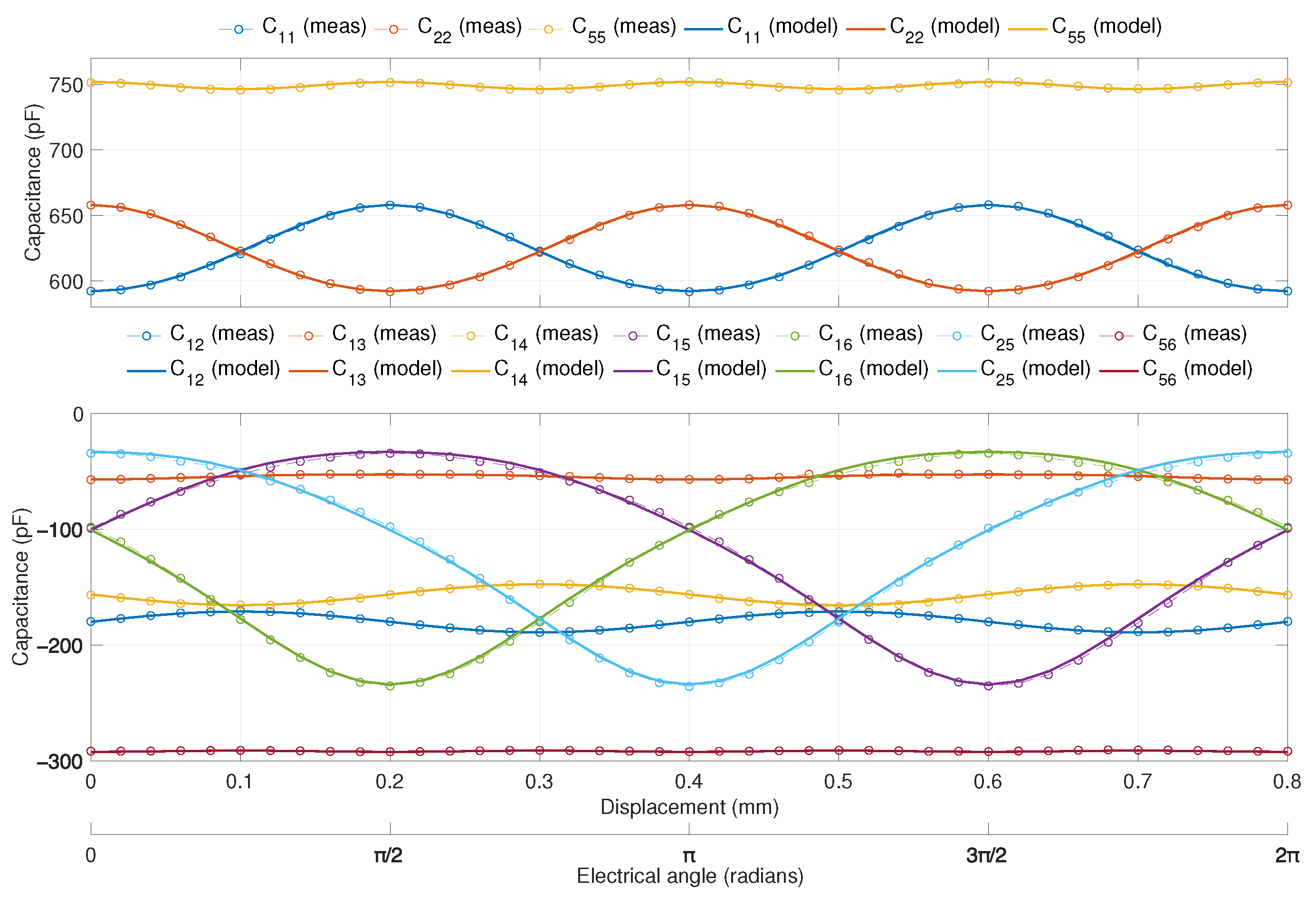
The reason for the harmonics in the presented equations can be understood by considering the interactions between the different electrodes. For example, variations in slider self-capacitance, (5), result from the interaction of one slider electrode with each of the four stator electrodes, thus the resulting waveform appears as a simple 4th order harmonic. This also implies that the highest order harmonic to significantly affect the motor’s behavior should be the 4th, as it results from the interaction of a single electrode moving across the largest possible number of electrodes in a single period. This is consistent with the fact that for the 3-phase motor, harmonics up to the 3rd order were observed [32]. The same logic applies to the capacitance between the slider electrodes, (8); this value is expected to be mostly constant, with small fluctuations resulting from the interaction with stator electrodes, again resulting in harmonics of the 4th order. This also generally follows for the stator capacitances, (4), (6) and (7). These should exhibit predominantly 2nd order harmonics, from the interactions with the slider electrodes. However, due to their relative proximity, they may also exhibit 4th order harmonics, as stator electrodes neighboring the considered electrode or pair interact with the slider. Last, in the case of (9), every harmonic up to the considered limit was included, as this was regarded as the capacitance with highest impact on the model outputs. While higher order harmonics may exist, they were disregarded, as their amplitude would be quite low, with their introduction significantly increasing the complexity of the model and delivering no practical benefit.
Following the protocol described in [32], the capacitance matrix was measured at 20 μm intervals for one cycle of electrodes (0.8 mm) for the prototype motor described in the experimental section. The markers in Figure 2 show the measured capacitance elements. Then, these capacitance variations were approximated using the functions (4) to (9). For approximation, some simplifications were applied which will be described in the next subsection. The solid lines in Figure 2 show the approximated results. With the designated harmonics, each capacitance element was approximated with high accuracy.
Different capacitance offsets were found among some elements that are expressed using the same approximating function. However, as these offsets (in other words, DC components) do not affect the calculations of the induced voltage and thrust force, the difference was ignored, and the average value was adopted when necessary.
2.3. Simplified Capacitance Identification
In measuring the capacitance matrix, while diagonal elements can be directly measured, non-diagonal elements can only be measured indirectly. Therefore, identification of the non-diagonal elements requires data conversions. For the approximations using (6) to (9), one can approximate the capacitance variations after converting all the measured data into the matrix elements, which has been done in the previous studies. This work, on the other hand, proposes approximating the variations before the data conversion.
In the measurement protocol described in [32], to identify the non-diagonal elements, , the value that can be first measured is
where is the direct measurement at position . Then, the non-diagonal element is recovered from this equation using diagonal elements, and , which are measured beforehand. This requires that all the discrete measurements be carried out at the same . Then, after repeating the data conversion for all the measurement points, we obtain the variation of the non-diagonal element, which is then approximated using (11).
In the protocol proposed in this paper, the approximation is done for . Then, the data conversion is done for the approximated functions, not for the value at each discrete point. This can considerably simplify the measurement, with no loss of accuracy, as the process is mathematically equivalent. As stated above, to obtain the matrix elements for discrete points, all the measurements need to be done exactly at the same positions, with the same density. In the proposed protocol, however, each capacitance can be measured at its own interval with different densities. The harmonics that need to be identified for each capacitance are shown in Table 1. Depending on the frequencies of the harmonics to be identified, the measurement densities can be adjusted to simplify the measurement. In this work, the approximations were performed by fitting to a sum of sinusoids, with frequencies constrained to the expected harmonics.
Accuracy for these fits was overall high, although lower for the lower amplitude measurements. We can consider normalized root mean square error (NRMSE) as a measure of fitting accuracy. This value was 6.47% and 8.11%, for the approximation of and , respectively, and ranged between 0.5% and 2.18% for the remaining measurements.
After obtaining the approximation for the directly measured capacitances, the conversions will be done for the approximated functions. This is equivalent to converting the coefficients in the following way.
3. Analysis of Motor Characteristics
3.1. Slider Voltage
In resonant induction electrostatic motors, slider voltage is determined by the motor’s properties and operating conditions, as it is induced on its electrodes and amplified by LC resonance. Slider voltages can be determined through equations relating the motor’s currents and voltages, as reported in [28]. Although mostly identical, the calculation procedure is described in this section, taking into account the new capacitance matrix as well as dielectric dissipation.
Let us consider a vector of the voltages on all the phases, contemplating the 4-phase stator and 2-phase slider, as
where corresponds to the stator voltage 0-pk amplitude, to its angular frequency and to the yet unknown slider voltage expression. The vector I of the current flowing into each electrode is written as
where the first term regards the current draw due to the motor’s capacitance, while the second is related to its losses, with as the dissipation factor for the dielectric materials. While the previous model did not explicitly consider the dissipation factor, including this term should enable more accurate voltage estimates, especially at lower resistance values.
Considering also the impedance of an inductor, , between the slider’s phases, slider voltage is given as
with the impedance of the inductor expressed as , where R is its series resistance and L its inductance.
The function expresses a complex number, which effectively defines the voltage amplification due to resonance. However, it does not represent final voltage amplitude, as this value also requires contributions of and , the magnitude of which depends on displacement. The phase of , , can be used as an expression of the motor’s resonant state. If the motor is at resonance this value should oscillate around , unless the resistance R is too large.
The motor’s resonant frequency can be approximated using the inductance value L as well as capacitance as
as long as the R is relatively low. This means that, for this motor, resonant frequency will depend on displacement, although the amplitude of this variation is expected to be small.
For comparison, the equivalent equation for slider voltage found in the previous work takes the form [28]
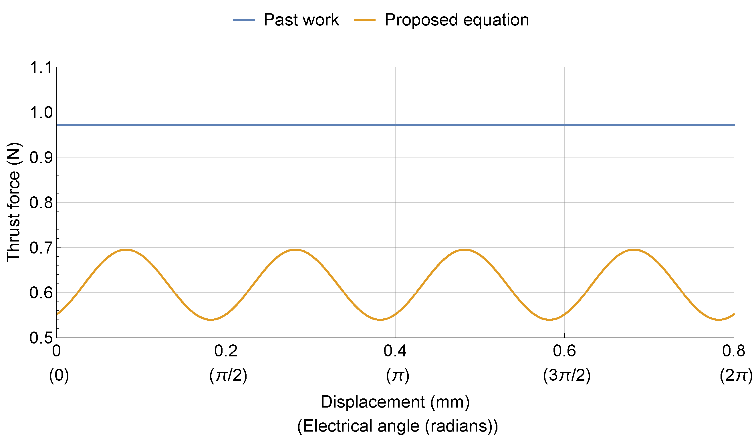
Both of these functions output complex numbers, the magnitude of which corresponds to the 0-pk amplitude of the time based voltage waveform. This quantity is useful for further analyses and can be defined as . A plot comparing the amplitudes for both versions of the function can be seen in Figure 3. The parameters used for these plots are indicated in Table 2, where f is the stator voltage frequency, so that .
The plot shows that, for the new equation, the slider voltage amplitude fluctuates with changes in displacement, which does not happen with the previous definition. The difference in mean value is largely due to the explicit consideration of the dissipation factor. If the dissipation loss is included in the resistance R, the average values for both models will be identical.
3.2. Thrust Force
For thrust force calculation, we can again follow the procedure from [28]. Motor thrust force can be obtained through the principle of virtual work, using the sinusoidal form for the voltage vectors, taken as their real component:
The direct result of solving (22) includes several frequency dependent sinusoidal terms. The purely electrical part of the motor, i.e., the resonating circuit, can respond to these high frequencies, which is observed as voltage amplification. On the other hand, these frequencies will be filtered out by the mechanical response. This means these terms will have to be eliminated from the thrust force equation. For this reason, there is a need to separate the resonant circuit frequency terms from the ones that will directly appear in the mechanical response (and need to be eliminated). This can be accomplished by redefining the slider voltage as in (24), by using and . Thus, by solving (22) and performing the aforementioned eliminations, we obtain
This equation should be valid as long as the driving frequency is sufficiently high (>10 kHz). Once more, for comparison, the equivalent equation in the literature [28] is
where corresponds to the slider voltage phase imposed by the resonant condition, taking the value of if the motor is at resonance.
A plot of the output of the two versions of the equation can be seen on Figure 4, again using the parameters in Table 2. The value for in (26) was calculated from (21). Again, the difference in the mean values is due to the explicit consideration of the dielectric dissipation. If it is included in R of the previous model, the average force of the two models will be the same. The plot shows that the equation introduced in this paper presents a force ripple that fluctuates with displacement, while the previous one shows no such variation.
An interesting point is that while the fluctuation of the voltage, in Figure 3, is about 10% of the average value, the fluctuation of the force reaches nearly 25% of its average. This implies that the effect of the harmonics in the capacitance variations is twofold for the induction motor. In case of dual excitation motors, the slider voltage is directly fed from amplifiers, and thus there is no fluctuation in the voltage amplitude. Nevertheless, the motor shows force ripple if there are capacitance harmonics. This is because the force depends on the derivative of the capacitance along the motion direction, as (22) shows; if there are harmonics, they will directly impact the output force. In addition to this effect, in the induction motor, the slider voltage amplitude fluctuates due to the capacitance harmonics. As the force is proportional to the product of the stator and slider voltages, the voltage fluctuation also results in force ripple. In such a way, the harmonics have a double effect on the force ripple of the induction motor. This shows an importance to analyze the force ripple in more detail.
3.3. Force Ripple Analysis
The ripple observed in the thrust force equation can have a negative impact on motor performance. As such, it should be analyzed for better understanding of its makeup and how it can be mitigated. To this end, a short numerical analysis is conducted in this section, using the parameters in Table 2, with the exception of the resistance value, which was set at 100 Ω.
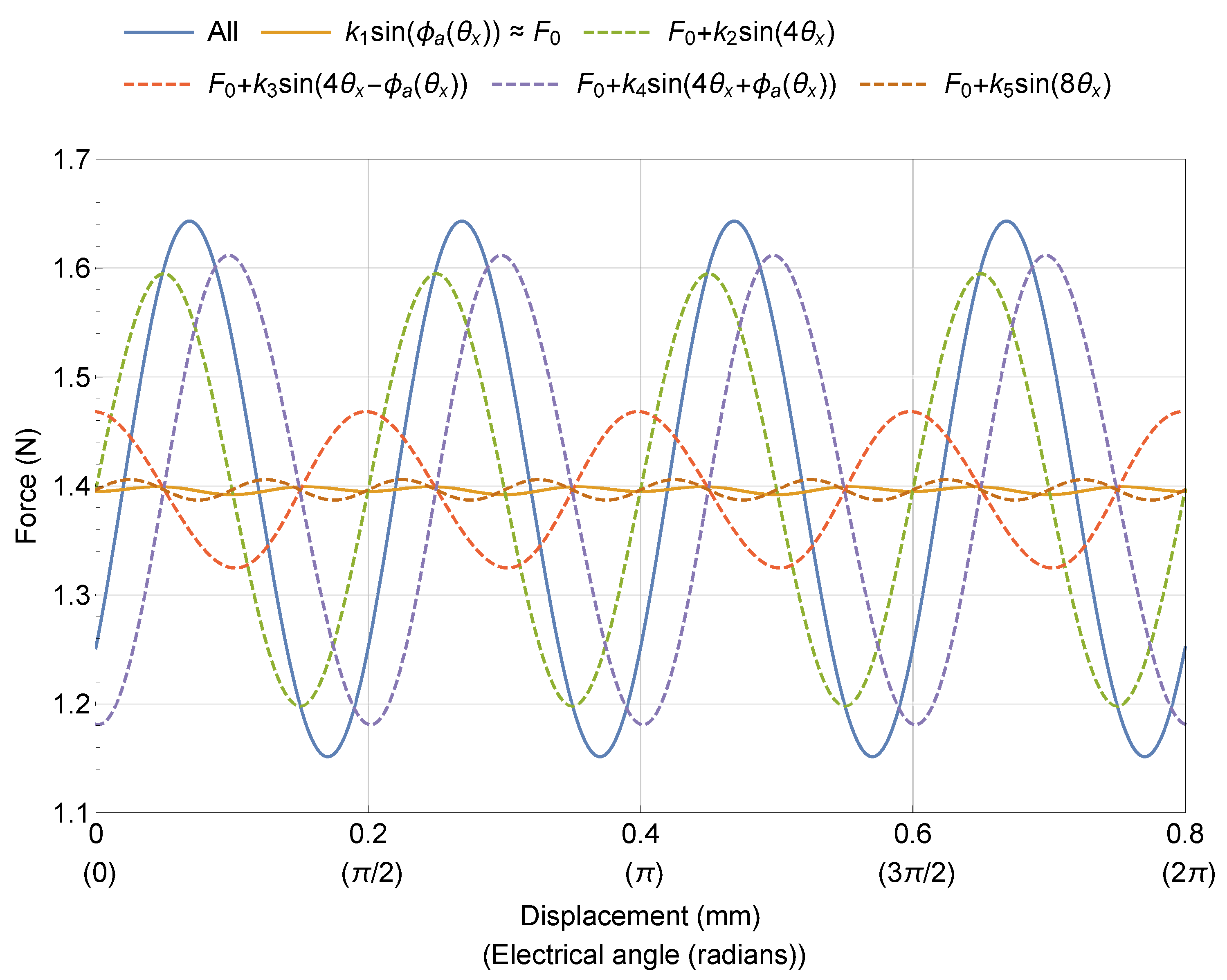
Figure 5 shows a decomposition of (25), evidencing the impact of each harmonic component of the force, over one displacement period of the motor. Each of the dashed lines in this plot corresponds to one term from (25), with the solid line corresponding to the total output. The effect of the 4th harmonics is clear, with the 8th harmonic essentially negligible. The force offset is provided by the sin term. As changes with displacement, it is not constant. However, if the motor is at resonance, this phase can be approximated as and the term considered constant with low loss of accuracy.
Furthermore, considering the plot on Figure 5, the values on Table 3, as well as (25), we can also remark on the impact of the higher order harmonic components of the capacitance coefficients in thrust force production. The 3rd capacitance harmonic is responsible for the existence of the terms of thrust force, given their multiplicative nature. As can be seen in Figure 5, these terms generate significant force ripple. The most relevant force harmonic with contributions by 4th order capacitance harmonics is the term. Here, and have a multiplicative effect on the square of the 1st and 3rd harmonics. This establishes their effect as non-negligible. Still, what we can call the stator 4th order harmonics, and do have a negligible effect, given their magnitude and the fact that they are only multiplied by the square of stator voltage, resulting in a term several orders of magnitude below mean force.
For further analysis, we can define percentage of force ripple, , from the quotient between the 0-pk force amplitude and mean force over a displacement period, :
which can now be analyzed as an output of the model. This value is likely to depend on a number of factors, such as capacitance harmonics’ amplitude and operating frequency. However, one that we can analyze is the variation with the ratio between slider and stator voltage amplitude, or voltage ratio. This ratio is expected to affect force ripple, because the different harmonic components that comprise thrust force are affected differently by each of the voltage amplitudes, as per (25).
Considering the motor at resonance, this parameter can be set by the resistance between the slider terminals. Figure 6 shows how the slider voltage ratio changes with resistance, as well as its effect on overall force ripple. As it can be seen, for the set operating conditions, the ripple appears to decrease asymptotically towards approximately 11%. Assuming this general trend holds for different conditions, the force ripple remains almost constant for voltage ratios of one or lower. Therefore, by setting the voltage ratio to one, we can suppress the force ripple to nearly the minimum, while keeping the overall thrust force.
On the other hand, this motor’s force is theoretically maximized at a voltage ratio of 2, considering that the slider electrodes would withstand twice higher voltage than the stator electrodes due to the twice longer electrode pitch. Thus, the voltage ratio should be carefully chosen considering the trade-off between the force magnitude and its ripple.
4. Experimental Validation
4.1. Experimental Setup
To evaluate the proposed model behavior, a set of experiments were carried out on the current motor prototype. Although, for simplicity, referred to as a prototype throughout this text, our test motor was built as a proof-of-concept device, designed for easy testing of the films’ performance, namely, force production at different positions. It has proved sufficiently robust to endure several rounds of testing with no major mechanical or electrical issues. The prototype comprises two electrostatic motor films: one stator and one slider, with active areas of 56.6 mm × 104 mm and 184 mm × 50 mm, respectively, and thickness of approximately 70 μm in these regions. During operation, the overlapping area corresponds to the lower value for each dimension, or 104 × 50 .
The setup can be seen in Figure 7. The stator film is secured to a base part through its non-active area, using screws and custom-made plastic supports. These also ensure film flatness. The base part also acts as a container for dielectric liquid, ensuring that both films can remain submerged during operation. The slider film is likewise attached to a supporting part, which also serves as a guide, sliding along the container walls with low friction. It also includes a tensioning mechanism to ensure the slider film remains flat during operation. The slider film is attached to this part in a similar fashion to the stator, using external supports secured with screws.
For inductance, a custom-wound ferrite cored inductor was used. It was assembled using a PQ 50/50 set, comprising a plastic former (B65982E, TDK, Tokyo, Japan), and matching ferrite core (B65981A, TDK). Due to the voltages reached by the slider during the experiments, the inductor was also immersed in dielectric fluid, to minimize corona discharge into the air, help prevent discharge between adjacent loops and also improve cooling. At ambient temperature, a frequency of 27 kHz, and while submerged in the liquid, it exhibited an inductance of 56.76 mH and series resistance of 109.4 Ω, as measured by an impedance analyzer. For some of the experiments, additional cement resistors were connected in series to the inductor. Current on this circuit loop was measured by a current probe (TCP312A, Tektronix, Beaverton, OR, USA), connected to a compatible amplifier (TCPA300, Tektronix).
The driving circuit consists of a function generator (NG1200, Yokogawa, Tokyo, Japan), followed by two stages of amplification. The first consists of a pair of high speed voltage amplifiers (4020, NF Corporation, Kanagawa, Japan)and the second a pair of purpose-built transformers. The function generator outputs two sinusoidal signals at 90° phase shift, within a range of 0 to 10 V0-pk. The first amplification stage amplifies these signals by 40 times, while the second splits them into four phases, and further amplifies the signal for each phase by 8 times. The phase-splitting is achieved by center-tapping the secondary windings of the transformers and connecting the center terminal to electrical ground. The outputs of this driving system are four electrical signals with identical frequency and amplitude, phase shifted from each other by 90°.
For force measurement, a load cell (LVS-1KA, Kyowa, Tokyo, Japan)mounted on a micropositioning stage was used, along with an amplifier module (DPM-711B, Kyowa). These were connected to an oscilloscope (DSO-X 200-A, Agilent Technologies, Santa Clara, CA, USA), which was also used for measurement of slider and stator voltages and acquisition of current.
4.2. Experimental Procedure
The experiments detailed in this section aimed to verify whether the model could adequately represent the variations in the motor’s slider voltage and thrust force with displacement. Overall, the experimental procedures consisted of driving the motor at its perceived resonant frequency, and measuring the relevant quantities for different positions of the slider. The experiment was performed several times, both using only the inductor for resonance, as well as with added resistance. All the measurements were done in a static situation, where the slider speed was zero. However, we confirmed that the slider could be actuated in the given conditions.
With the slider placed against the load cell, stator voltage amplitude and frequency were set. Resonant frequency was determined by changing the driving frequency on the function generator, selecting the frequency that resulted in the highest voltage amplitude. Stator voltage, , was adjusted so as to ensure that the achieved resonant voltage was within the safe operating limits of the prototype (under 1800 V0-pk). The system was set up so that the motor applied force towards the load cell, mounted on a micrometric positioning stage. Throughout the experiment, the load cell was moved in discrete increments of approximately 20 μm, across a full displacement period. This movement was in the same direction as the force application, i.e., moving the load cell away from the motor. Each value was captured after a few seconds of stabilization time.
For each sample, driving frequency, stator and slider voltage, as well as inductor current were acquired. The obtained waveforms were also used to calculate resistance and inductance across the slider terminals. Using the slider voltage and inductor current RMS values ( and , respectively) and phase difference between them (), resistance, R, and inductive reactance, , can be directly calculated, with inductance, L, calculated from the latter:
This procedure allowed all model parameters to be measured during the experiments, with the exception of . This parameter would be very hard to measure during the experiment, and even beforehand it can be challenging. As this value is associated with each capacitance parameter, its proper inclusion would require considering the interaction between its various instances, as well as displacement variation. For these reasons, this value was inferred for each data set. For each experiment, the value was set so that the mean slider voltage produced by the model was as close as possible to the measured value. As this value was considered independently of resistance, we were also able to ensure that the inferred values are physically plausible.
4.3. Experimental Results
The most relevant measurements are plotted in Figure 8. The negative displacement is due to the movement direction, which was opposite to when measuring capacitance. Regarding thrust force, the absolute value is shown.
The outputs of the model were plotted considering two different sets of parameters, presented in Table 3 and identified as (i) and (ii). The first set comprises the measured values as detailed in the previous section. Set (ii) replaces the measured inductance value with an “optimized” alternative, which is an inductance value that enables the best possible matching of the slider voltage waveforms, with the also readjusted to compensate for changes in voltage magnitude. This optimized value was not determined for the conditions of experiment (c), as the data did not allow any further optimization. For this experiment, the results of the past model were included for comparison.
The results show a good match with the models, in terms of frequency components, for both voltage and force measurements. There is also general agreement between the shape of the voltage waveforms for all experiments. While there is a greater difference in the case of the force measurements, the overall results still suggest that the model adequately characterizes the tested motor. Furthermore, it can be seen that the use of the adjusted inductance value produced a considerably more accurate force output for case (a), and mitigated the phase error in (b).
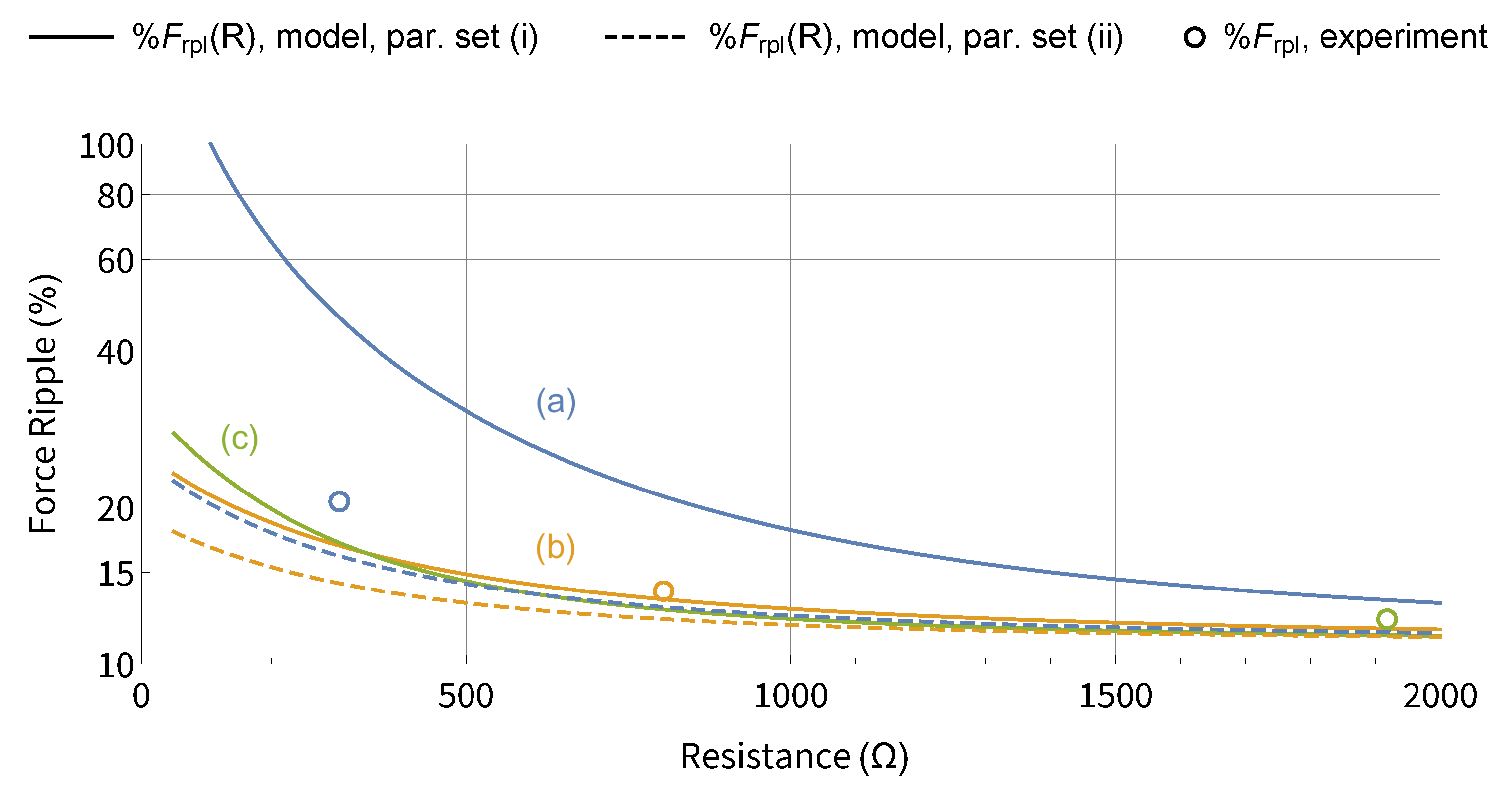
In addition, the force ripple for these results can also be calculated from (27) and plotted against the resistance value, along the expected results for the model considering different sets of parameters. In order to minimize effects of drift, the force ripple was calculated between adjacent peaks and averaged for each experiment. This is presented in Figure 9. The plots are color coded, so that each color illustrates one “experiment”, as per the rows in Table 2. The results show that the resulting force ripple measured in the experiments appears to follow the predicted trend, with its values close to those predicted by the model, especially for the two latter experiments. These results are in accordance with those presented in Figure 8, with the largest discrepancy occurring between experiment (a) and the model output using measured parameters (parameter set (i)).
5. Discussion
5.1. General Model Evaluation
The results suggest that the newly developed model better describes the motor’s operation. Although a greater number of experiments is necessary for properly establishing its accuracy, it confirms the advantages of considering higher-order capacitance harmonics for this motor. However, this representation is not perfectly accurate. In this particular kind of motor, there are several important sources of error, which hinder its accurate modeling. For example, the gap length between the stator and the slider would not be constant during operation, due to fluctuations in slider voltage. As the capacitance of the motor considerably depends on the gap length, the change in the gap length would cause capacitance error. Nevertheless, with the exception of experiment (a), the model output tracks the experimental results relatively closely, suggesting the capacitance error may in practice have been rather low. To better evaluate this, we can plot the relative error with displacement for each experiment and for both model conditions. This plot can be seen in Figure 10. This better illustrates the improvements in model tracking upon adjustment of the inductance value, with (a) going from over 100% relative error at some points, to approximately . The results for experiment (c) further confirm what had been seen in the previous section, that the model tracking error under these conditions is reasonably low, under if we ignore drift, likely caused by changes in temperature of the different components during operation.
In the case of experiment (b), the model results using the measured values exhibit a small, but noticeable phase error relative to the measured points, which is almost eliminated when the “optimized” inductance value is used. The presence of a phase difference indicates a difference in resonance frequency between the model and the prototype, which would mean the model output was calculated using incorrect values of inductance, capacitance or operating frequency. While the improvement in results with the change of inductance may suggest this was the cause of error, it may also indicate a capacitance error, given their similar contribution to resonance.
5.2. Mean Force Changes with Inductance
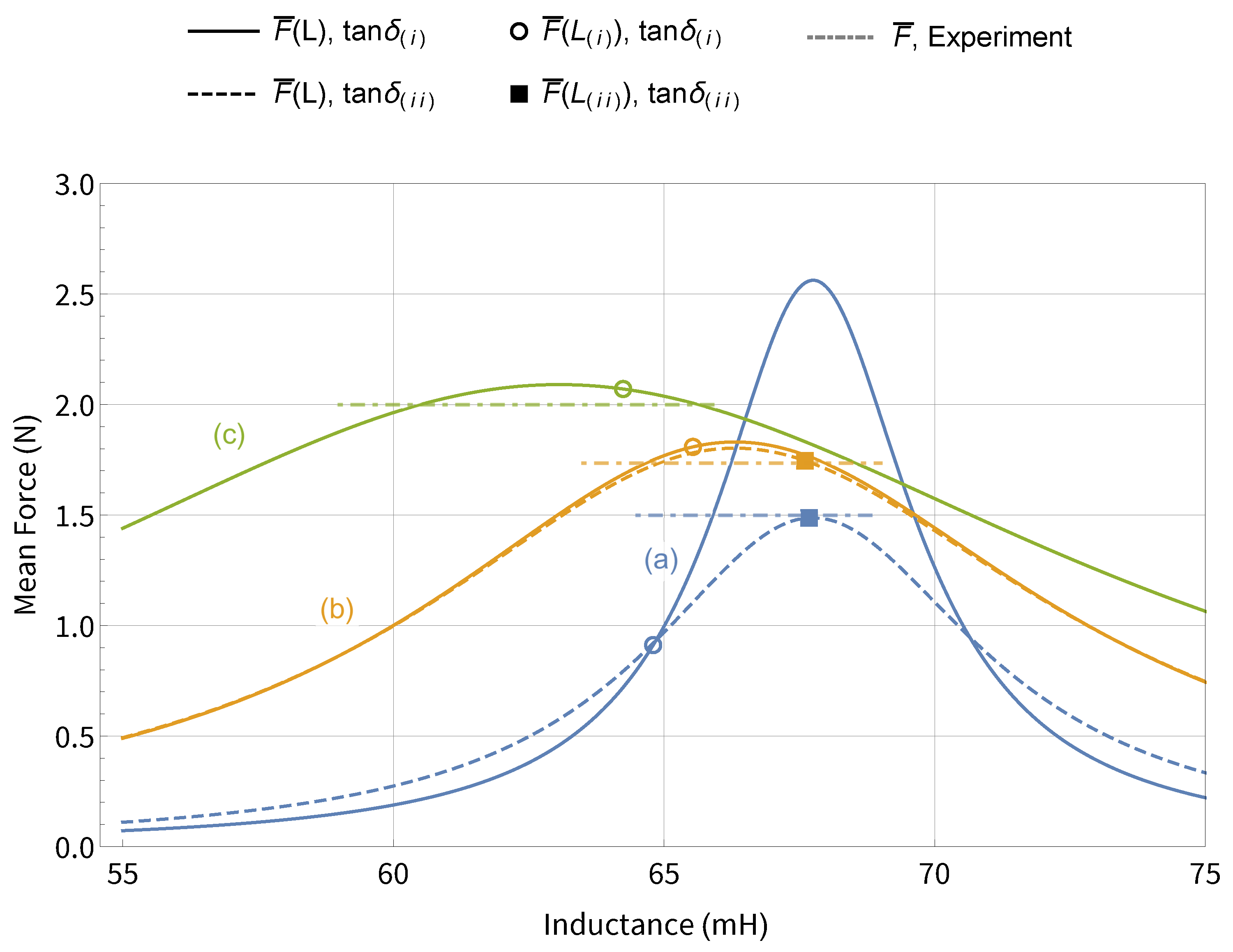
To further expand on this last point, we can examine the differences in error between the three sets of model/experiment, by analyzing how mean force changes with inductance for each set of experimental conditions. As mentioned before, this can also be interpreted as a force/capacitance relationship, given their similar contribution to resonance.
Figure 11 shows a plot of mean force () as a function of inductance for the different model conditions, with the relevant inductance values identified along the curves. The experimentally measured mean forces are also presented as horizontal lines, for comparison.
As resistance has a flattening effect on the voltage resonance curves, and thrust force is proportional to slider voltage, this effect can be seen to transfer to the plotted output. This shows that a small error in the considered inductance value can have a varying effect on calculated force depending on the resistance, potentially explaining the difference between the model output for experiments (a) and (b). The same 3 mH difference in inductance can be responsible for a change of mean force of over 0.5 N or under 0.1 N, depending on the considered model parameters. Likewise, the results should be similar if we consider changes in capacitance. This also demonstrates another advantage of using higher resistance values for resonance. Besides decreasing force ripple, it enables a flatter resonant peak, making force levels more robust against changes in operating conditions. This is important, especially as slider voltage frequency is known to change in dynamic conditions [26], not treated in this paper.
5.3. Force Ripple
Regarding the force ripple results, shown in Figure 9, these are also mostly in agreement with the analysis in Figure 10. The largest discrepancy between the experimental data and model outputs is seen in experiment (a) and the lowest in experiment (c). One notable exception is for the results regarding experiment (b). For these, a higher force ripple error is observed when considering the “optimized” model. This is explained by the fact that the error between experiment (b) and the model with measured parameters was mostly a phase error, which is disregarded in the force ripple calculations. Bearing this in mind, if we consider the most accurate results to be those obtained with the parameter set (ii), we can observe that the experimental results are consistently to the right of the model plots. Although part of this error is likely attributable to other sources, as already discussed, this may also imply that the measured resistance value is actually higher than the effective value during the experiments. As was inferred for all model plots, and its contribution to the model outputs is similar to that of resistance, it is possible that some of the error in resistance was compensated. Furthermore, given that resistance and inductance were calculated from the same measured quantities, this would also suggest a likely degree of error with the inductance measurement. This complements the discussion on Section 5.2, supporting that at least part of the reason why the inferred inductance values show better results may be due to error in its measurement. Nevertheless, the experimental results were, qualitatively, in good accordance with the model. This verifies the correctness of the proposed model. However, because of the difficulty of precise parameter estimations, the results were slightly deviated from the theoretical estimation. This may be resolved in the future with better parameter measurements at the experimental conditions and stabilization of these conditions, namely, in terms of operating temperature.
5.4. General Comment
The overall consistency between the model and the experimental results implies that the capacitance harmonics have a non-negligible effect on the motor behaviour. The fact that this was not witnessed in the original prototype [28] leads us to believe this effect is likely due to differences of the films, namely, electrode widths, as well as substrate thickness, which affects the gap between stator and slider electrodes. The films in the current prototype were designed and manufactured more recently, with a lower overall thickness. This suggests that force ripple is adjustable by changing these parameters, so as to decrease the effects of the capacitance harmonics. This is a matter that will have to be addressed in future research.
In light of the obtained results, the proposed model appears to be a useful extension to the available tools to describe the behaviour of resonant electrostatic induction motors. As a broader model, it should comprise a good starting point for future studies. The achieved force error, particularly for the experiments where higher resistance was used, is still reasonably low for this kind of motor, especially considering the complexity of the new model. While at this point it is difficult to rigorously judge the accuracy of the model itself, given the uncertainty around the values of most parameters, the reported results suggest it properly reflects the motor’s operation.
6. Conclusions and Future Work
This paper reports the definition of a new model for 2–4 phase resonant electrostatic induction motors, exhibiting changes in slider voltage and thrust force with displacement, compatible with experimental observations. This model is important to better understand the expected output of such a motor, assisting in future designs and development of control algorithms. Likewise, having a defined protocol for formulation of such a model is also valuable, allowing future researchers to more quickly react to changes in parameters that might arise in future prototypes.
The model appears to describe the experimental behaviour of the motor, namely, in terms of voltage and force ripple, which were absent from past literature for induction electrostatic film motors. Regarding its accuracy, it is acceptable for most cases, although it appears to be limited by uncertainty around parameter values, such as inductance, resistance and the capacitance coefficients themselves at the experimental conditions.
In the future, more extensive testing should be performed to further understand the limitations of this model. More accurate measurement of all the relevant parameters at the experimental conditions would also be beneficial to understanding any possible modeling errors. Furthermore, despite the higher complexity of this model, there are still some aspects which could be augmented, such as considering fluctuations in gap thickness. Last, research into means of minimizing force ripple is also necessary, as the current values might limit the practical applications of this motor.
Author Contributions
Conceptualization, F.C., M.O. and A.Y.; methodology, F.C.; validation, F.C., G.Z. and A.Y.; investigation, F.C.; writing—original draft preparation, F.C.; writing—review and editing, F.C., G.Z., M.O., S.Y. and A.Y.; supervision, S.Y. and A.Y. All authors have read and agreed to the published version of the manuscript.
Funding
This research received no external funding.
Conflicts of Interest
This work was conducted in collaboration between The University of Tokyo and Honda R&D Co., Ltd.
References
- Gao, Z.; Shi, Q.; Fukuda, T.; Li, C.; Huang, Q. An overview of biomimetic robots with animal behaviors. Neurocomputing 2019, 332, 339–350. [Google Scholar] [CrossRef]
- Li, T.; Li, G.; Liang, Y.; Cheng, T.; Dai, J.; Yang, X.; Liu, B.; Zeng, Z.; Huang, Z.; Luo, Y.; et al. Fast-moving soft electronic fish. Sci. Adv. 2017, 3, e1602045. [Google Scholar] [CrossRef] [PubMed] [Green Version]
- Wan, C.; Gorb, S.N. Body-catapult mechanism of the sandhopper jump and its biomimetic implications. Acta Biomater. 2021, 124, 282–290. [Google Scholar] [CrossRef]
- Wu, Y.; Yim, J.K.; Liang, J.; Shao, Z.; Qi, M.; Zhong, J.; Luo, Z.; Yan, X.; Zhang, M.; Wang, X.; et al. Insect-scale fast moving and ultrarobust soft robot. Sci. Robot. 2019, 4, eaax1594. [Google Scholar] [CrossRef] [PubMed] [Green Version]
- Gu, G.; Zou, J.; Zhao, R.; Zhao, X.; Zhu, X. Soft wall-climbing robots. Sci. Robot. 2018, 3, eaat2874. [Google Scholar] [CrossRef] [PubMed] [Green Version]
- Cao, J.; Qin, L.; Liu, J.; Ren, Q.; Foo, C.C.; Wang, H.; Lee, H.P.; Zhu, J. Untethered soft robot capable of stable locomotion using soft electrostatic actuators. Extrem. Mech. Lett. 2018, 21, 9–16. [Google Scholar] [CrossRef]
- Jafferis, N.T.; Helbling, E.F.; Karpelson, M.; Wood, R.J. Untethered flight of an insect-sized flapping-wing microscale aerial vehicle. Nature 2019, 570, 491–495. [Google Scholar] [CrossRef]
- Kim, S.; Laschi, C.; Trimmer, B. Soft robotics: A bioinspired evolution in robotics. Trends Biotechnol. 2013, 31, 287–294. [Google Scholar] [CrossRef] [PubMed]
- Robla-Gomez, S.; Becerra, V.M.; Llata, J.R.; Gonzalez-Sarabia, E.; Torre-Ferrero, C.; Perez-Oria, J. Working Together: A Review on Safe Human-Robot Collaboration in Industrial Environments. IEEE Access 2017, 5, 26754–26773. [Google Scholar] [CrossRef]
- Coltelli, M.A.; Catterlin, J.; Scherer, A.; Kartalov, E.P. Simulations of 3D-Printable biomimetic artificial muscles based on microfluidic microcapacitors for exoskeletal actuation and stealthy underwater propulsion. Sens. Actuators A Phys. 2021, 325, 112700. [Google Scholar] [CrossRef]
- Wang, E.; Shu, J.; Jin, H.; Tao, Z.; Xie, J.; Tang, S.Y.; Li, X.; Li, W.; Dickey, M.D.; Zhang, S. Liquid metal motor. iScience 2021, 24, 101911. [Google Scholar] [CrossRef]
- Kim, W.; Byun, J.; Kim, J.K.; Choi, W.Y.; Jakobsen, K.; Jakobsen, J.; Lee, D.Y.; Cho, K.J. Bioinspired dual-morphing stretchable origami. Sci. Robot. 2019, 4, eaay3493. [Google Scholar] [CrossRef] [PubMed]
- Liu, Q.; Zuo, J.; Zhu, C.; Xie, S.Q. Design and control of soft rehabilitation robots actuated by pneumatic muscles: State of the art. Future Gener. Comput. Syst. 2020, 113, 620–634. [Google Scholar] [CrossRef]
- Villoslada, A.; Flores, A.; Copaci, D.; Blanco, D.; Moreno, L. High-displacement flexible Shape Memory Alloy actuator for soft wearable robots. Robot. Auton. Syst. 2015, 73, 91–101. [Google Scholar] [CrossRef]
- Koh, J.S.; Cho, K.J. Omegabot: Biomimetic inchworm robot using SMA coil actuator and smart composite microstructures (SCM). In Proceedings of the 2009 IEEE International Conference on Robotics and Biomimetics (ROBIO), Guilin, China, 19–23 December 2009. [Google Scholar] [CrossRef]
- Li, W.B.; Zhang, W.M.; Gao, Q.H.; Guo, Q.W.; Wu, S.; Zou, H.X.; Yan, H.; Peng, Z.K.; Meng, G. Electrostatic field induced coupling actuation mechanism for dielectric elastomer actuators. Extrem. Mech. Lett. 2020, 35, 100638. [Google Scholar] [CrossRef]
- Adachi, M.; Moroka, H.; Kawamoto, H.; Wakabayashi, S.; Hoshino, T. Particle-size sorting system of lunar regolith using electrostatic traveling wave. J. Electrost. 2017, 89, 69–76. [Google Scholar] [CrossRef]
- Duduta, M.; Wood, R.J.; Clarke, D.R. Multilayer Dielectric Elastomers for Fast, Programmable Actuation without Prestretch. Adv. Mater. 2016, 28, 8058–8063. [Google Scholar] [CrossRef]
- Leng, J.; Liu, Z.; Zhang, X.; Huang, D.; Qi, M.; Yan, X. Design and analysis of a corona motor with a novel multi-stage structure. J. Electrost. 2021, 109, 103538. [Google Scholar] [CrossRef]
- Ge, B.; Ludois, D.C. Dielectric liquids for enhanced field force in macro scale direct drive electrostatic actuators and rotating machinery. IEEE Trans. Dielectr. Electr. Insul. 2016, 23, 1924–1934. [Google Scholar] [CrossRef]
- Schaler, E.W.; Zohdi, T.I.; Fearing, R.S. Thin-film repulsive-force electrostatic actuators. Sens. Actuators A Phys. 2018, 270, 252–261. [Google Scholar] [CrossRef]
- Niino, T.; Egawa, S.; Higuchi, T. High-power and high-efficiency electrostatic actuator. In Proceedings of the IEEE Micro Electro Mechanical Systems, Fort Lauderdale, FL, USA, 10 February 1993; pp. 283–291. [Google Scholar] [CrossRef]
- Egawa, S.; Higuchi, T. Multi-layered electrostatic film actuator. In Proceedings of the IEEE Proceedings on Micro Electro Mechanical Systems, An Investigation of Micro Structures, Sensors, Actuators, Machines and Robots, Napa Valley, CA, USA, 11–14 February 1990; pp. 166–171. [Google Scholar]
- Niino, T.; Higuchi, T.; Egawa, S. Dual excitation multiphase electrostatic drive. In Proceedings of the IAS’95. Conference Record of the 1995 IEEE Industry Applications Conference Thirtieth IAS Annual Meeting, Orlando, FL, USA, 8–12 October 1995. [Google Scholar] [CrossRef]
- Yamamoto, A.; Nishijima, T.; Higuchi, T.; Inaba, A. Robotic arm using flexible electrostatic film actuators. In Proceedings of the 2003 IEEE International Symposium on Industrial Electronics (Cat. No.03TH8692), Rio de Janeiro, Brazil, 9–11 June 2003; Volume 2, pp. 940–945. [Google Scholar]
- Hosobata, T.; Yamamoto, A.; Higuchi, T. An electrostatic induction motor utilizing electrical resonance for torque enhancement. Sens. Actuators A Phys. 2012, 173, 180–189. [Google Scholar] [CrossRef]
- Hosobata, T.; Yamamoto, A.; Higuchi, T. Modeling and Analysis of a Linear Resonant Electrostatic Induction Motor Considering Capacitance Imbalance. IEEE Trans. Ind. Electron. 2014, 61, 3439–3447. [Google Scholar] [CrossRef]
- Takei, K.; Yamamoto, A. Modeling of voltage induction of a resonant electrostatic induction motor using 2-phase slider and a single coil. In Proceedings of the 2016 IEEE/SICE International Symposium on System Integration (SII), Sapporo, Japan, 13–15 December 2016; pp. 260–265. [Google Scholar] [CrossRef]
- Carneiro, F.; Osada, M.; Zhang, G.; Yoshimoto, S.; Yamamoto, A. Achieving Resonance with Piezoelectric Transducers on 2–4 Phase Resonant Electrostatic Induction Motors. In Proceedings of the 2021 IEEE International Conference on Mechatronics (ICM), Kashiwa, Japan, 7–9 March 2021. [Google Scholar] [CrossRef]
- Carneiro, F.; Osada, M.; Zhang, G.; Yoshimoto, S.; Yamamoto, A. Increasing Thrust Force on 2–4 Phase Resonant Electrostatic Induction Motors through Stacking. In Proceedings of the IECON 2020 The 46th Annual Conference of the IEEE Industrial Electronics Society, Singapore, 18–21 October 2020. [Google Scholar] [CrossRef]
- YAmashita, N.; Yamamoto, A.; Higuchi, T. Effects of Electrode Configuration for Performances of Voltage-Induction-Type Electrostatic Motors. J. Adv. Mech. Des. Syst. Manuf. 2013, 7, 333–347. [Google Scholar] [CrossRef] [Green Version]
- Yamamoto, A.; Niino, T.; Higuchi, T. Modeling and identification of an electrostatic motor. Precis. Eng. 2006, 30, 104–113. [Google Scholar] [CrossRef]
Figure 1.
Schematic images of the 2–4 phase resonant electrostatic induction motor: (a) the general layout of the films; (b) their typical arrangement, external circuit components and working principle; and (c) a more detailed section view with identification of the discrete capacitive elements (designations are the ones introduced in this paper).

Figure 2.
Capacitance versus displacement, for different elements of the capacitance matrix (indices indicate position within the matrix).
Figure 2.
Capacitance versus displacement, for different elements of the capacitance matrix (indices indicate position within the matrix).

Figure 3.
Comparison of the voltage amplitude output, as a function of displacement, between the newly proposed equation and the one reported in [28].
Figure 3.
Comparison of the voltage amplitude output, as a function of displacement, between the newly proposed equation and the one reported in [28].

Figure 4.
Comparison of the thrust force output, as a function of displacement, between the newly proposed equation and the one reported in [28].
Figure 4.
Comparison of the thrust force output, as a function of displacement, between the newly proposed equation and the one reported in [28].

Figure 5.
Model thrust force output throughout one displacement period, considering different force harmonic components. The coefficient represents the amplitude of each harmonic, as per (25). The average value of is defined as , which is equal to and is approximately 1.4 N.
Figure 5.
Model thrust force output throughout one displacement period, considering different force harmonic components. The coefficient represents the amplitude of each harmonic, as per (25). The average value of is defined as , which is equal to and is approximately 1.4 N.

Figure 6.
Voltage amplitude ratio and as a function of resistance with resistance (in the range of 10 to 5000 Ω), for the considered model parameters. was calculated for , for which its value is maximum.
Figure 6.
Voltage amplitude ratio and as a function of resistance with resistance (in the range of 10 to 5000 Ω), for the considered model parameters. was calculated for , for which its value is maximum.

Figure 7.
Experimental setup used for force measurement. (a) Prototype motor and load cell assembly. (b) Pictures of the used films, highlighting the electrode structure.
Figure 7.
Experimental setup used for force measurement. (a) Prototype motor and load cell assembly. (b) Pictures of the used films, highlighting the electrode structure.

Figure 8.
Main force and voltage measurement results and comparison to the two model implementations: (i), using measured inductance values and (ii), using “optimized” inductance values. (a) Using only the inductor (R ≈ 305 Ω). (b) With external resistance connected in series (R ≈ 804 Ω). (c) With external resistance connected in series (R ≈ 1918 Ω). Model (ii) was not generated for this set of results. Results using past model included for comparison.


Figure 9.
Force ripple measurements compared to values obtained from the model under different conditions.
Figure 9.
Force ripple measurements compared to values obtained from the model under different conditions.

Figure 10.
Relative error for both model parameter sets on the performed experiments. Error relative to past model also presented for experiment (c). Cyan-colored lines indicate error.
Figure 10.
Relative error for both model parameter sets on the performed experiments. Error relative to past model also presented for experiment (c). Cyan-colored lines indicate error.

Figure 11.
Comparison of mean force output against inductance, considering different sets of model parameters.
Figure 11.
Comparison of mean force output against inductance, considering different sets of model parameters.


Table 1.
Identified offsets and harmonic amplitudes used in the definition of the equations that compose the capacitance matrix.
Table 1.
Identified offsets and harmonic amplitudes used in the definition of the equations that compose the capacitance matrix.
| Measured Capacitance † | Offset | 1st | 2nd | 3rd | 4th |
|---|---|---|---|---|---|
| (1,1), (2,2), (3,3), (4,4) | – | – | |||
| (5,5), (6,6) | – | – | – | ||
| (1,2), (1,4), (2,3), (3,4) | – | – | |||
| (1,3), (2,4) | – | – | |||
| – | – | ||||
| (5,6) | – | – | – |
† Only the upper triangular elements are specified.
Table 2.
Parameters used for calculations of model outputs. Capacitance values expressed in pF.
| (V) | p (mm) | L (mH) | R (Ω) | tan δ | f (kHz) | |||
|---|---|---|---|---|---|---|---|---|
| 500 | 0.2 | 66.6 | 800 | 0.04 | 27 | |||
| 115.1 | 95.6 | 4.88 | 291.8 | 0.506 | 749.1 | 2.82 | 0.401 | 1.32 |
Table 3.
Parameters used for the motor model when comparing with experimental results. Values within parenthesis indicate total measured range.
Table 3.
Parameters used for the motor model when comparing with experimental results. Values within parenthesis indicate total measured range.
| Exp. | Parameter Set | Experimentally Measured | Inferred | Model | ||||
|---|---|---|---|---|---|---|---|---|
| R (Ω) | L (mH) | (V) | (kHz) | L (mH) | tan δ | (kHz) | ||
| (a) | (i) | 304.8 (7.3–650.2) | 64.80 (63.87–65.31) | 550 | 26.80 | – | 0.00585 | 27.38 |
| (ii) | 67.68 | 0.02935 | 26.80 | |||||
| (b) | (i) | 804.2 (420.9–1207) | 65.53 (65.16–65.93) | 840 | 27.10 | – | 0.035 | 27.31 |
| (ii) | 67.60 | 0.03665 | 26.88 | |||||
| (c) | (i) | 1918 (1548–2297) | 64.244 (63.55–64.94) | 1205 | 27.80 | – | 0.0172 | 27.75 |
| (ii) | – | – | – | |||||
Publisher’s Note: MDPI stays neutral with regard to jurisdictional claims in published maps and institutional affiliations. |
© 2021 by the authors. Licensee MDPI, Basel, Switzerland. This article is an open access article distributed under the terms and conditions of the Creative Commons Attribution (CC BY) license (https://creativecommons.org/licenses/by/4.0/).
Share and Cite
MDPI and ACS Style
Carneiro, F.; Zhang, G.; Osada, M.; Yoshimoto, S.; Yamamoto, A. An Extended Model for Ripple Analysis of 2–4 Phase Resonant Electrostatic Induction Motors. Actuators 2021, 10, 291. https://0-doi-org.brum.beds.ac.uk/10.3390/act10110291
AMA Style
Carneiro F, Zhang G, Osada M, Yoshimoto S, Yamamoto A. An Extended Model for Ripple Analysis of 2–4 Phase Resonant Electrostatic Induction Motors. Actuators. 2021; 10(11):291. https://0-doi-org.brum.beds.ac.uk/10.3390/act10110291
Chicago/Turabian StyleCarneiro, Fernando, Guangwei Zhang, Masahiko Osada, Shunsuke Yoshimoto, and Akio Yamamoto. 2021. "An Extended Model for Ripple Analysis of 2–4 Phase Resonant Electrostatic Induction Motors" Actuators 10, no. 11: 291. https://0-doi-org.brum.beds.ac.uk/10.3390/act10110291
Note that from the first issue of 2016, this journal uses article numbers instead of page numbers. See further details here.