
Deviation Sequence Neural Network Control for Path Tracking of Autonomous Vehicles


1
Xiamen King Long United Automotive Industry Co., Ltd., Xiamen 361021, China
2
College of Mechanical Engineering and Automation, Huaqiao University, Xiamen 361021, China
*
Author to whom correspondence should be addressed.
Actuators 2024, 13(3), 101; https://0-doi-org.brum.beds.ac.uk/10.3390/act13030101
Submission received: 19 January 2024
/
Revised: 3 March 2024
/
Accepted: 3 March 2024
/
Published: 5 March 2024
(This article belongs to the Section Actuators for Land Transport)
Abstract
:Despite its excellent performance in path tracking control, the model predictive control (MPC) is limited by computational complexity in practical applications. The neural network control (NNC) is another attractive solution by learning the historical driving data to approximate optimal control law, but a concern is that the NNC lacks security guarantees when encountering new scenarios that it has never been trained on. Inspired by the prediction process of MPC, the deviation sequence neural network control (DS-NNC) separates the vehicle dynamic model from the approximation process and rebuilds the input of the neural network (NN). Taking full use of the deviation sequence architecture and the real-time vehicle dynamic model, the DS-NNC is expected to enhance the adaptability and the training efficiency of NN. Finally, the effectiveness of the proposed controller is verified through simulations in Matlab/Simulink. The simulation results indicate that the proposed path tracking NN controller possesses adaptability and learning capabilities, enabling it to generate optimal control variables within a shorter computation time and handle variations in vehicle models and driving scenarios.
1. Introduction
Path planning and tracking control are fundamental and important components of autonomous vehicles (AVs). An investigation in reference [1] highlights that the research topic of path tracking has significantly grown in recent years. For secure and efficient driving, autonomous vehicles need to track precisely the reference trajectory generated by the path planning module. In the past years, to improve the path tracking control performance of AVs, many significant results have been reported with the applications of advanced linear and nonlinear control techniques, such as PID [2,3], LQR [4,5], MPC [6,7] and SMC [8,9]. Model predictive control (MPC) is a highly competitive solution with respect to the other possible control technologies [1]. An advantage is the better tracking performance during high speed and medium-to-high lateral acceleration conditions, compared to the kinematic or geometry-based path tracking methods, such as the pure pursuit [10] and Stanley [11] methods. Furthermore, the capability of managing multi-variable problems and systematically considering constraints on states and control actions make it an ideal choice for multiple-input multiple-output (MIMO) systems, e.g., for AVs with multiple actuators.
Despite its various advantages in path tracking control, MPC is limited by computational cost of the online solution in real-time applications [12,13]. As the system dimension and predictive horizon expand, the resulting exponential growth in computational complexity for solving the optimal control problem (OCP) severely consumes computing resources. The last generations of solvers and control hardware solutions have helped to mitigate the problem. For example, qpOASES speed-up the QP solution based on tracing the solution along a linear homotropy between a QP problem with known solution and the QP problem to be solved [14]. In addition, the custom solver can also compute control actions faster than the conventional method [15,16].
Considering the requirement of real-time, offline methods is another solution for the path tracking control of AVs. Explicit MPC (EMPC), which determines the control law by designing a piecewise affine function over polyhedral regions, has been implemented in various fields [17,18,19]. Typically, computing the control variable from the piecewise affine function is faster than solving the QP online. EMPC is verified as the optimal control law for linear time-invariant (LTI) systems [20]. However, the vehicle dynamic model is not time-invariant but varies with changes in longitudinal velocity and sideslip angle. The piecewise affine function cannot cover all conditions and thus, the optimal control solutions may not be obtained with the piecewise affine function designed by the preset condition.
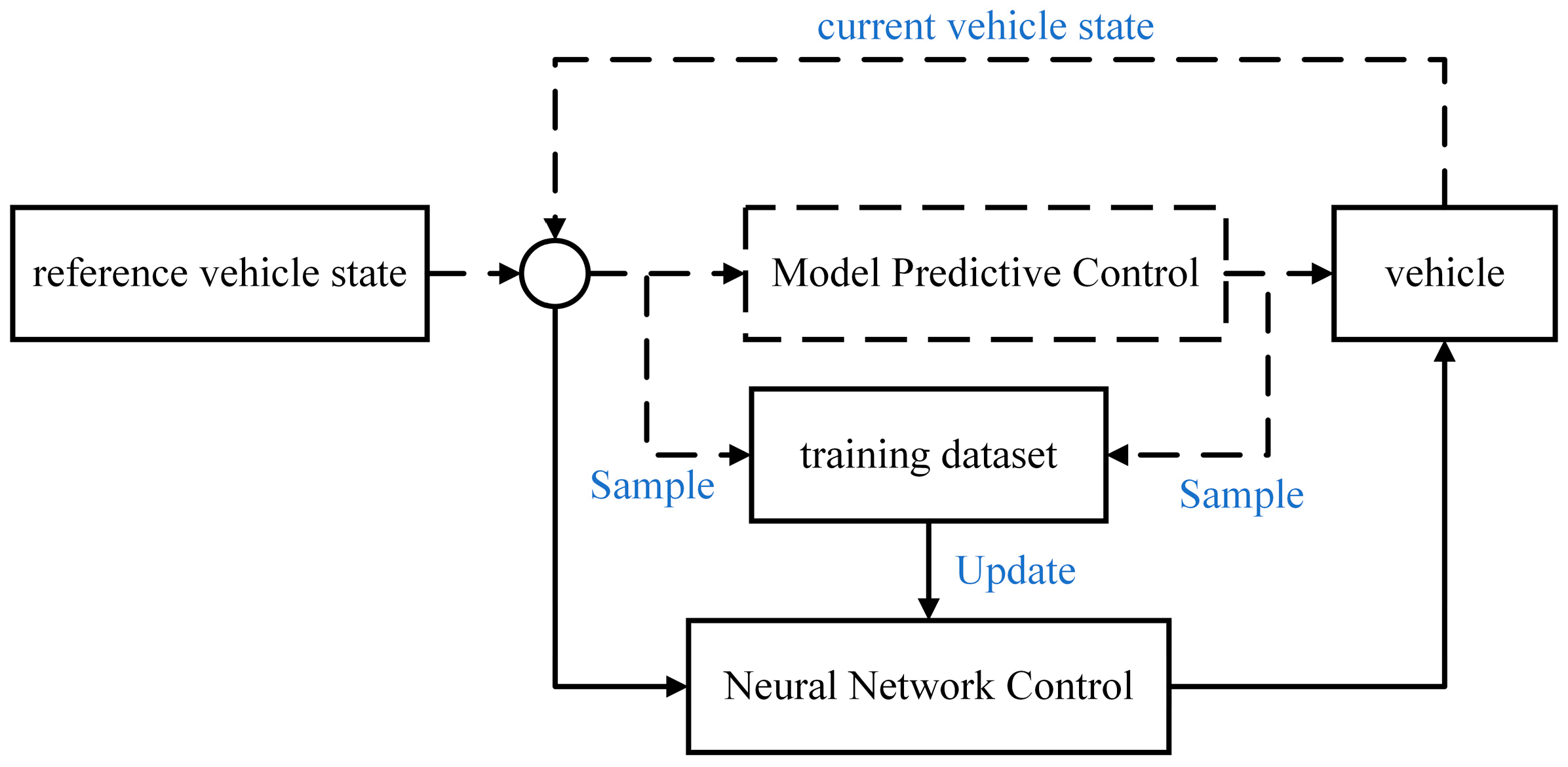
It is noteworthy that practical AVs involve a large amount of repetitive maneuvers in certain circumstances, such as racing or parking [21]. Therefore, it is possible to take the advantages of system repetition and in turn, improve the tracking performance based on the historical driving data [22], which motivates learning-based control techniques. The general framework of neural network control (NNC) is shown in Figure 1. In this framework, the conventional MPC computes the optimal control law and generates the training dataset. Generally, the training dataset contains system state and corresponding optimal control variables in each sample time. Next, NN is used to fit training data generated by sampling the original controller many times and the result is applied “as is” to replace the controller. The NNC trained on the dataset is expected to simulate the optimal solving process. NNC offers unique advantages, including employing simple mathematical expressions and possessing excellent approximation capacity. More importantly, unlike the exponential increase in computational burden experienced by MPC, the computational demand of NNC grows moderately as the system complexity rises. Compared to EMPC, NNC does not use the dynamic model directly. As a result, it alleviates the adverse effect brought by time-variant parameters.
One of the earliest applications of artificial neural networks to the vehicle control problem was the autonomous land vehicle in a neural network (ALVINN) system by Pomerleau in 1989 which was first described in [23]. That neural network has a 30 × 32-neuron input layer, one 4-neuron hidden layer and a 30-neuron output layer. In the ALVINN system, the neural network is provided with image information from a camera together with the steering commands of the human driver and then generates discrete steering action. The neural networks utilized in early works are significantly smaller when compared to what is feasible with today’s technology [24]. End-to-end learning, where observations are mapped directly to low-level vehicle control interface commands, is a popular approach for plants of different complexity. Mariusz et al. [24] trained a convolutional neural network (CNN) to map raw pixels directly from a single front-facing camera to steering commands. The inputs for the end-to-end learning network are not limited to image information. For longitudinal speed control of a vehicle, the error between the speed output command and the actual speed is a reasonable input [25]. Ghoniem et al. [26] introduced a suspension controller to generate a valve opening signal. Similarly, the input of NNC is the error between road input and suspension displacement. Direct state information is an effective input, but for complex tasks, such as autonomous driving, the diversity of the data set should be ensured if the aim is to train a generalizable model which can drive in all different environments [27]. Furthermore, a concern is that NNC lacks security guarantees when encountering new scenarios that it has never been trained on. The new scenarios not only represent a different steering angle and velocity, but also represent different vehicle parameters such as sprung mass and yaw inertia moment. Feature engineering, where the training data generated by running the original controller are used to craft artificial features that serve as inputs to the NN approximation, is a promising approach to improve generalization. The training still occurs via pure regression and the crafting of features can include the use of inputs that are not ever presented to the original MPC controller.
For large scale MIMO control problems in the building sector, Drgoňa et al. [28] introduced a versatile framework for mimicry of the behavior of optimization-based controllers. The approach employs deep time delay neural networks (TDNN) and regression trees (RT) to derive the dependency of multiple control inputs on parameters. Karg and Lucia [29] consider as input data the parameters of the mixed-integer quadratic programs (MIQPs) and as output data the first element of the optimal solution. In addition to approaches that directly redesign the inputs of NN, creating addition features is also effective. Lovelett et al. [30] used state feedback to project the system’s position in state space onto a latent manifold, and then estimated the optimal control policy. By leveraging such a lowdimensional structure of the control policies, simple functions can be found to approximate the control law using fewer training data points.
Recent studies offer various types of approaches to realize feature engineering. However, predictive sequence is still an MPC factor that is not fully considered. In this paper, the deviation sequence neural network control (DS-NNC) is presented for AVs. In order to enhance the adaptability to a time-variant dynamic model and various scenarios, DS-NNC separates the vehicle dynamic model from the approximation process and rebuilds the input of the neural network. Finally, the effectiveness of the proposed controller is verified through simulations in Matlab/Simulink.
2. Deviation Sequence Neural Network Control
2.1. Reformulation of Approximate Function
Considering a mapping from current vehicle state vector xk (longitudinal velocity and yaw rate) and reference vehicle state vector rk to control variable uk, a general structure of NN controller generates the control law with the form below:
As is shown in Figure 2, this mapping is expected to simulate the optimal solving process where the vehicle controller generates the optimal control variables. Unfortunately, the state variable xk is not suitable as an input variable. The reason is that the values of the vehicle state can vary significantly, making it challenging for the function to accommodate all the data generated from the optimal control law in simulations. Another concern is overfitting. Due to the limited availability of abundant training data, the neural network can only perform well in a few specific scenarios. What is worse, this problem becomes more severe when the NN is trained perfectly, but solely for that particular dataset. In order to make it more suitable for a vehicle controller, some improvement is presented as follows.
If one hypothesizes that a multi-layer neural network can approximate F1(xk, rk), then it is equivalent to hypothesize that they can asymptotically approximate part of this function, i.e., the following:
where the variable E represents the deviation sequence and the second equation is based on the explicit calculation process from the discrete system state-space equation to the deviation sequence. This reformulation is motivated by considering of the known relationship between the current vehicle state vector xk and the reference vehicle state vector rk to the error sequence vector E. In other words, this improvement integrates prior knowledge (the established vehicle dynamic model) into the architecture of NN control rather than letting NN approximate the real-time vehicle dynamic model. A similar concept is physics-informed machine learning (PINN) which integrates (noisy) data and mathematical models, and can be trained from additional information obtained by enforcing the physical laws [31,32]. So rather than expect an NN to approximate F1, we explicitly let these layers approximate the simplified function F2. Although both forms can be asymptotically approximate (as hypothesized), the ease of learning might be different. From another perspective, the relation between control output and error is similar in different scenarios. Remarkably, the premise of this assumption is that the vehicle is stable. Therefore, the deviation form represents more various scenarios compared with the function F1 of which the input is the current vehicle state and reference vehicle state. It is unlikely that the deviation sequence is optimal, but our reformulation may help to reduce the impact of model change and extend the working range of the NN controller.
2.2. Implementation
The precondition to train the NN controller is the dataset. In this paper, the training data are sampled from a complete model predictive control process. First, the vehicle dynamic model is described, followed by the deviation model and the path tracking control problem formulation. In addition, some details about the improvement of the proposed NN controller are illustrated.
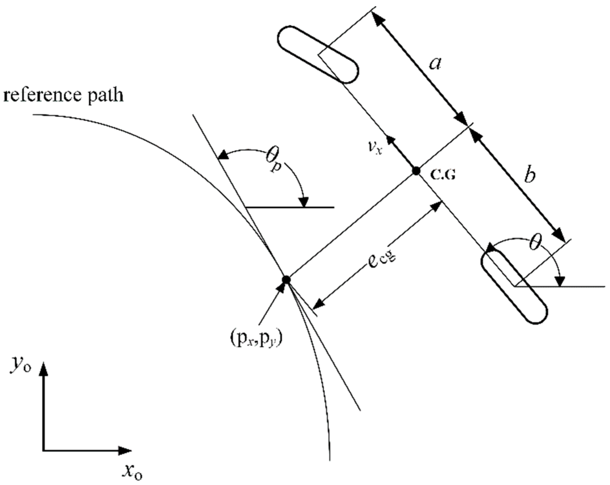
For simplicity, the single-track model is used to describe vehicle dynamics. This form is the most commonly used when designing the vehicle lateral controller because it contains the necessary elements to describe the lateral motion. Figure 3. shows the schematic of this model. In this model, the vehicle dynamic can be modeled in the non-linear form of the equations of motion. Because of the complexity of non-linear equations, the design of an MPC controller is difficult. In addition, the sideslip stiffness of a turning vehicle changes greatly and the tire parameters depend heavily on the road surface and environmental conditions [33]. To estimate the system state accurately, the nonlinear equations derived from basic principles of dynamics are linearized based on two assumptions, i.e., unchanged vehicle velocity and linear tire sideslip characteristics. The linear mathematic expression of the vehicle single-track model is shown as (3):
Here cr is the cornering stiffness of the rear axle, cf is the cornering stiffness of the front axle, vx and vy are the vehicle longitudinal and lateral velocity respectively, m is the vehicle mass, r is the yaw rate, a is the distance from the front axis to the center of gravity, b is the distance from the rear axis to the center of gravity, Iz is the vehicle yaw inertia. The control variables δf and ΔMz represent the front wheel steering angle and the additional yaw moment generated by the differential moment of the wheel, respectively.
As mentioned earlier, the deviation form represents various scenarios. In the path tracking scenario, the deviation model can better describe the changes in vehicle state. As shown in the Figure 4, considering a preset reference trajectory, the deviation variables are built as follows:
where ecg represents the distance between the vehicle centroid and the closest point in the reference path, eθ represents the error between the heading angle of the vehicle direction and the heading angle of the closest point, r(s) is the reference yaw rate.
By combining Equations (3) and (4), the deviation tracking control model can be described as follows:
To facilitate the controller design and analysis, we reformulate Equations (5) and (6) with the state variables into a linear state-space equation:
where the state variable vector is modelled as
and the control variable vector is modelled as follows:
The system matrix and input matrix are given by the following:
The matrix C comes from the definition of the heading angle error eθ as shown in (4) and is given by the following:
To predict the future state, the discrete form of the Equation (7) is as follows:
where Ak and Bk represent the discrete system matrix and control matrix respectively. At each time step k, the predictive system state sequence vector
can be derived by the p-step recursive calculation of the discrete system transition Equation (13). The calculation process is shown as follows:
For simplification, Equation (15) is integrated into the matrix form (16):
The matrix Ψ is given by
The matrix Θ1 is given by
The matrix Θ2 is given by
Considering a reference vehicle state sequence
in the next p time step, the predictive deviation sequence
is obtained. Here r is the vector which consists of the reference sideslip angle and the reference yaw rate. In path tracking, the reference is set to zero to minimize the tracking deviation. Remarkably, the reference sequence vector must be given before calculating the control law and is generally generated by route planning.
In the MPC process, the OCP is solved at each time instant to output the control variable sequence vector Uk:
subject to the system state transition function (13) and the limits of the actuators
where T represents the equivalent torque applied to the tires. In the optimization problem (23),
is the control output sequence vector which can be the combination of tracking error, control effort, energy cost, or other factors. The metrics Q and W are used to weigh the deviation from the state error and the value of the control vector, respectively, when the importance of state variables is different. Several solution methods exist for the optimization problem (22), including interior point methods, active set methods, gradient projection methods, and dual methods. Each method has its advantages and application range, with the choice of method often depending on the specific problem characteristics, size, and solving requirements. Among these methods, interior point methods (IPMs) provide advantages in constraint handling, global convergence, scalability, flexibility, and parameter tuning in MPC. These advantages make IPMs an effective solution method widely applied in MPC.
In Equation (21), the control variables sequence vector is a variable before the solving process. Because the variable is not allowed in the input of NN, the control variables sequence vector Uk should be separated from (21), despite it being the basic element of the optimal process. The predictive deviation sequences
represents theoretically the predictive state sequence when the vehicle is running without control. This form does not contain any variable and could be calculated by the deviation model (13) and current vehicle state xk. Finally, Equation (2) is reformulated as follows:
By learning the mapping F2 from the sample dataset, the proposed DS-NNC approximates the optimal control variables, namely, the front wheel steering angle and the additional yaw moment in this work, to track currently the reference path.
In the next section, we show the process of training the neural network and deploy the trained network on the car to verify the effectiveness.
3. Results
First, a closed-loop path, which consists of various scenarios, is designed for the verification of the proposed path tracking controller. As shown in Figure 5, the test car starts from the position (0,0) to the positive direction of the X-axis and tracks this path under the control of the conventional MPC controller. At the end of the path, the MATLAB profiler is expected to record the simulation data which contain the vehicle state (longitudinal speed and yaw rate), control variables (front wheel steering angle and additional yaw moment), and the execution time of each module. The vehicle parameters adopted in simulations are presented in Table 1. All the simulations are performed in MATLAB2022a on a 16 GB RAM desktop PC with Intel i5-12490 CPU.
The neural network comprises a three-layer fully connected architecture, each layer featuring 40 neurons. The input layer receives a p-dimension prediction deviation sequence vector, where p denotes the predictive horizon length. The output is the control variable vector, encompassing the normalized front wheel steering angle and additional yaw moment, balanced to the same magnitude scale pre-training to mitigate scale discrepancies.
The dataset sampled from simulation process is divided into two parts for the training process of the NN controller. Specifically, we train the same NN controller on the whole dataset, the first half dataset, and the second half dataset, respectively. This design aims at verification of the guarantee on system safety, especially when the proposed NN controller encounters a new scenario that has never been trained on. When it is implemented in the path tracking on the whole path, the NN controller trained on the partial dataset will face scenarios that it has never experienced. The backpropagation (BP) algorithm is one of the most commonly used training methods for neural networks with excellent fitting precision, and was adopted to train the NN in this work.
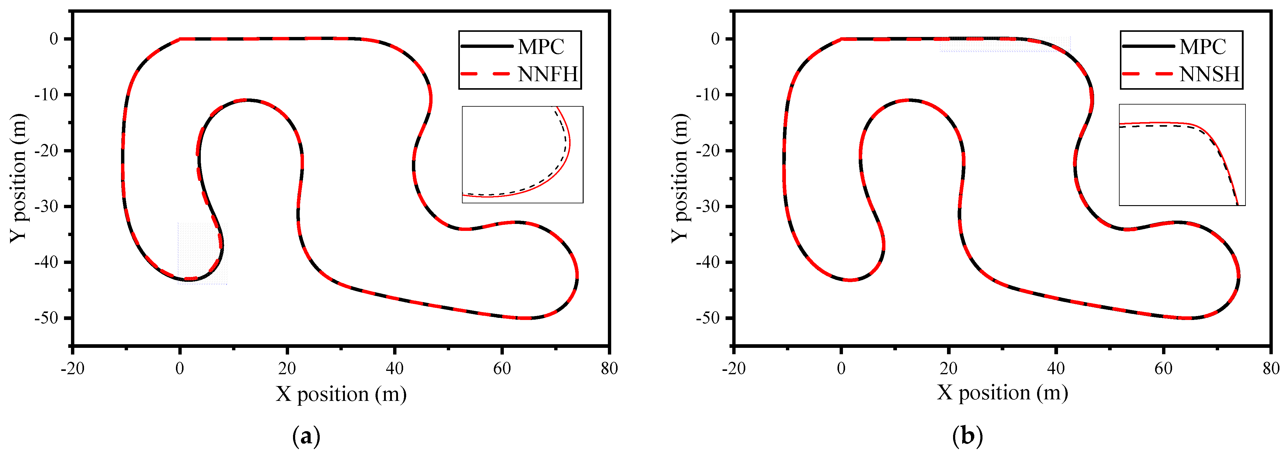
The simulation results are presented in Figure 5 and Figure 6 and Table 2 and Table 3. We have two major observations from this result. First, the vehicle under the control of the three NN controller tracks the reference path accurately. More importantly, this advantage in tracking capability does not come at the cost of high computational power consumption. The trained NN controller could generate the control variables at a speed of ten times or more than the MPC (Table 3).
As the baseline controller, the mean tracking error of MPC is 0.2236 m in the whole path. Here the tracking error is calculated by the following:
Comparing with the MPC controller, the proposed NN controller reaches a lower level of 0.2234 m. Figure 5 and Figure 6 show an interesting result. Despite the partial train data, the NN controller has a better tracking performance. In the first half of the tracking trajectory, the average tracking error of the NN trained on the second half dataset (NNSH) is 0.05 less than that of the MPC. Similarly, the NN trained on the first half dataset (NNFH) has lower error level in the second half of the tracking trajectory. One underlying reason for this issue is the utilization of root mean square (RMS) as the primary performance metric during the training process. As a result, when encountering input, which it has never seen before, the network is inclined to generate outputs based mainly on its experience with similar inputs, potentially limiting its effectiveness in dealing with novel situations. The phenomenon raises an issue in that only when the coverage rate of conditions is high enough, can the adaptiveness of NNC be guaranteed. For logical completeness, further discussion is scheduled in the next case.
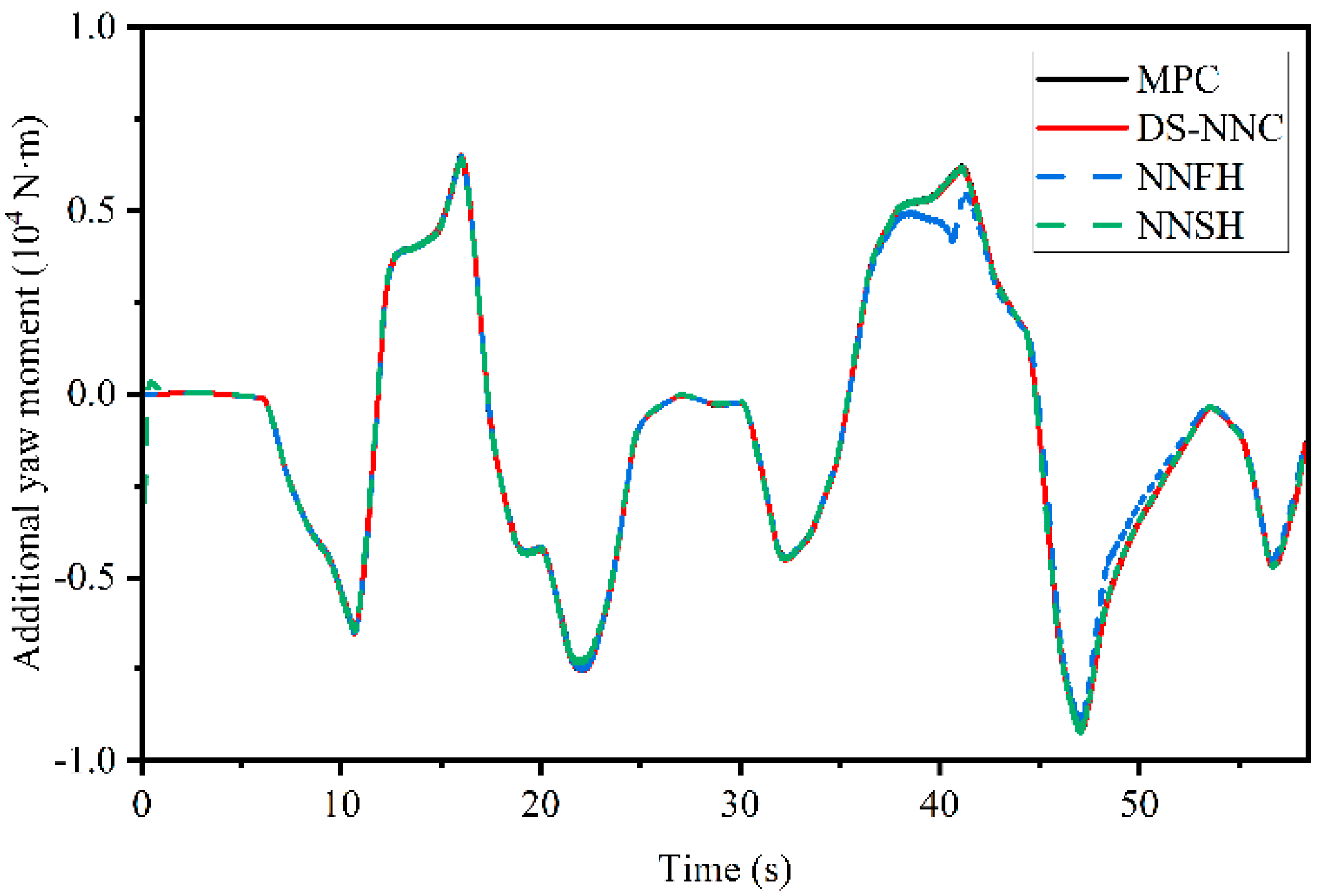
Second, compared to the baseline NN trained on the whole dataset, the NNFH and the NNSH show generalization when encountering a new scenario that has never been trained on. As is shown in Figure 7, Despite a small discrepancy, the NNFH performs better in the first half path than in the second half. Similarly, the NNSH has a greater tracking error when the car is running in the path that has never been trained before. In addition, the control variables and additional yaw moment, could better illustrate this phenomenon. As is shown in Figure 8, the additional yaw moment generated by the NNFH has a slight deviation from the baseline in the second half path tracking process. Although the overall imitation is good, some discrepancy appears in the expected position. Fortunately, this deviation has little impact on the tracking control.
With the purpose of further security verification of the NN controller in the face of unknown scenarios, the path and vehicle model are different in the next two cases. As shown in Figure 9, we design a bigger and more complex closed-loop path and keep the MPC and the NN controller with the same parameters (predictive horizon and control weight) as before. The vehicle longitudinal velocity is set to 18 km/h. The simulation result is shown in Figure 9, Figure 10 and Figure 11, including the tracking trajectories as well as the tracking error profiles for the lateral deviation and yaw angle error profiles. From the result of the tracking trajectories, an observation is that the MPC controller shows a gradually increasing error when the car runs in the second half of the path, while the NN controller tracks the reference path more currently. Furthermore, the tracking position error and the yaw angle error profiles in Figure 10 show a more detailed trend than in the last case. The tracking position error of the NN controller is around 1 m while that of MPC gradually rises to 14 m at the end of the path. In the different path, the tracking position error of the MPC is more significant. The increasing error is attributed to the unsuitable parameters. For example, an excessive predictive horizon can lead to increased sensitivity to model errors and less reliable control actions. As is mentioned in Section 2, the DS-NNC removes the control weight from the MPC architecture and reduces the impact of predictive horizon on control variable generation. Consequently, the DS-NNC can be implemented in various scenarios without redesigned parameters.
Next, we further explore the adaptiveness of the proposed NN controller for different vehicle models. Because the calculation of the input of the NN controller, i.e., predictive deviation sequence E, is independent of the network, the changes of the vehicle parameters can be considered as prior knowledge. In this case, the car is significantly lighter and shorter to ensure differentiation of the system model. The vehicle parameters are shown in Table 4 The vehicle mass is reduced by approximately 40% and the length is reduced by approximately 30%. Remarkably, we also use the same MPC controller and NN controller as before. The simulation result is shown in Figure 12 and Figure 13, including the tracking trajectories as well as the tracking profiles. Similarly, the MPC cannot still track the reference path currently as a result of the control parameters. Although the MPC is redesigned based on the new vehicle dynamic model, the inappropriate control parameters limit its accuracy. As a comparison, the proposed NN controller has a better tracking performance. At the end of the tracking trajectory, the tracking position error keeps below 0.5 m. The three cases show the tracking performance of the proposed DS-NNC. Although NNC can also approximate the original controller, DS-NNC has more generalization. A brief example in Figure 14 indicates that advantage.
4. Conclusions
This paper presents a deviation sequence neural network control (DS-NNC) for path tracking of AVs. The algorithm is based on offline sampling and rich data set, and the real-time computation time is reduced by 96%. The two significant parts are feature engineering and the improved structure of NNC, which allow more driving scenarios and provide more generalization. It can be summarized as follows:
- (1)
- Introducing the deviation sequence into the input structure of neural network control improves the generalization and reduces the model complexity and the training burden. As is shown in the theory analysis, it contains more driving scenarios and better future motion tendency and thus can represent multiple states.
- (2)
- The proposed structure separates the vehicle dynamic model from the approximation process and adds a computation module for the predictive state, making full use of the real-time vehicle dynamic model. Compared to directly approximating the mapping of states to control inputs, this structure reduces the complexity of the neural network training because it does not need to consider the dynamic model during the approximation process. Additionally, when the dynamic model is changed, an NN trained offline approximates an out-of-date dynamic model and results in an incremental tracking error. This error could be avoided.
In this paper, simulation experiments are conducted in two environments with different complexity levels in Matlab/Simulink. The simulation results indicate that the proposed path tracking controller possesses adaptability and learning capabilities, enabling it to generate optimal control variables within a shorter computation time and handle variations in vehicle models and driving scenarios.
In summary, the path tracking controller based on the proposed DS-NNC can improve the speed and adaptiveness. However, although most driving scenarios are covered, it is possible for a real-time controller to reach an unavailable state. Ideally, one would want an NNC that is a drop-in replacement for the original controller but runs faster and preserves all of its desirable features. For controllers that can already run in real time, hot starting has been proved to be a general and effective method with strict guarantee, where a conventional solver is still being used at every control iteration [34]. By themselves, the outputs of the network have no guarantees but because all primal variables are predicted, a simple algebraic check can be performed to assess the feasibility and suboptimality of the solution. Projecting onto feasible sets is another method [35]. This coercion preserves the recursive feasibility guarantees of MPC but requires significant overhead to perform the projection, and computation of the maximal control invariant set which is only feasible for some problems. These methods increase the computational burden to some extent, which runs counter to the purpose of neural network control. Additionally, the proposed DS-NNC loses some information on the weight matrix. In our simulations, general control parameters are chosen. This prevents the controller from improving to better performance. A promising approach would be the combination of weight matrix and deviation sequence. That may improve the performance in a large maneuver.
Author Contributions
Conceptualization, L.S. and Y.M.; methodology, Y.M.; software, Y.M.; validation, L.S. and Y.M.; formal analysis, F.Z.; investigation, F.Z. and Y.Z.; resources, B.L.; data curation, L.S.; writing—original draft preparation, Y.M.; writing—review and editing, L.S. and F.Z.; visualization, B.L.; supervision, F.Z. All authors have read and agreed to the published version of the manuscript.
Funding
This research was supported by the National Key Research and Development Program of China (2021YFB2500700).
Data Availability Statement
Data are contained within the article.
Conflicts of Interest
Authors Liang Su and Baoxing Lin were employed by the company Xiamen King Long United Automotive Industry Co., Ltd. The remaining authors declare that the research was conducted in the absence of any commercial or financial relationships that could be construed as a potential conflict of interest.
References
- Stano, P.; Montanaro, U.; Tavernini, D.; Tufo, M.; Fiengo, G.; Novella, L.; Sorniotti, A. Model predictive path tracking control for automated road vehicles: A review. Annu. Rev. Control 2022, 55, 194–236. [Google Scholar] [CrossRef]
- Han, G.; Fu, W.; Wang, W.; Wu, Z. The lateral tracking control for the intelligent vehicle based on adaptive PID neural network. Sensors 2017, 17, 1244. [Google Scholar] [CrossRef]
- Al-Mayyahi, A.; Wang, W.; Birch, P. Path tracking of autonomous ground vehicle based on fractional order PID controller optimized by PSO. In Proceedings of the 2015 IEEE 13th International Symposium on Applied Machine Intelligence and Informatics (SAMI), Herl’any, Slovakia, 22–24 January 2015; pp. 109–114. [Google Scholar]
- Xu, S.; Peng, H. Design, analysis, and experiments of preview path tracking control for autonomous vehicles. IEEE Trans. Intell. Transp. Syst. 2019, 21, 48–58. [Google Scholar] [CrossRef]
- Chatzikomis, C.; Sorniotti, A.; Gruber, P.; Zanchetta, M.; Willans, D.; Balcombe, B. Comparison of path tracking and torque-vectoring controllers for autonomous electric vehicles. IEEE Trans. Intell. Veh. 2018, 3, 559–570. [Google Scholar] [CrossRef]
- Peng, H.N.; Wang, W.D.; An, Q.; Xiang, C.L.; Li, L. Path Tracking and Direct Yaw Moment Coordinated Control Based on Robust MPC With the Finite Time Horizon for Autonomous Independent-Drive Vehicles. IEEE Trans. Veh. Technol. 2020, 69, 6053–6066. [Google Scholar] [CrossRef]
- Tian, Y.; Yao, Q.Q.; Wang, C.Q.; Wang, S.Y.; Liu, J.Q.; Wang, Q. Switched model predictive controller for path tracking of autonomous vehicle considering rollover stability. Veh. Syst. Dyn. 2022, 60, 4166–4185. [Google Scholar] [CrossRef]
- Zhang, X.; Zhu, X. Autonomous path tracking control of intelligent electric vehicles based on lane detection and optimal preview method. Expert Syst. Appl. 2019, 121, 38–48. [Google Scholar] [CrossRef]
- Zhang, Y.; Liu, K.; Gao, F.; Zhao, F. Research on path planning and path tracking control of autonomous vehicles based on improved APF and SMC. Sensors 2023, 23, 7918. [Google Scholar] [CrossRef]
- Gámez Serna, C.; Lombard, A.; Ruichek, Y.; Abbas-Turki, A. GPS-based curve estimation for an adaptive pure pursuit algorithm. In Advances in Computational Intelligence: 15th Mexican International Conference on Artificial Intelligence, MICAI 2016, Cancún, Mexico, October 23–28, 2016, Proceedings, Part I; Springer: Cham, Switzerland, 2016; pp. 497–511. [Google Scholar]
- Zhu, Q.; Huang, Z.; Liu, D.; Dai, B. An adaptive path tracking method for autonomous land vehicle based on neural dynamic programming. In Proceedings of the 2016 IEEE International Conference on Mechatronics and Automation, Harbin, China, 7–10 August 2016; pp. 1429–1434. [Google Scholar]
- Siampis, E.; Velenis, E.; Gariuolo, S.; Longo, S. A real-time nonlinear model predictive control strategy for stabilization of an electric vehicle at the limits of handling. IEEE Trans. Control Syst. Technol. 2017, 26, 1982–1994. [Google Scholar] [CrossRef]
- Lee, J.; Chang, H.-J. Analysis of explicit model predictive control for path-following control. PLoS ONE 2018, 13, e0194110. [Google Scholar] [CrossRef]
- Ferreau, H.J.; Kirches, C.; Potschka, A.; Bock, H.G.; Diehl, M. qpOASES: A parametric active-set algorithm for quadratic programming. Math. Program. Comput. 2014, 6, 327–363. [Google Scholar] [CrossRef]
- Richter, S.; Jones, C.N.; Morari, M. Real-time input-constrained MPC using fast gradient methods. In Proceedings of the 48th IEEE Conference on Decision and Control (CDC) Held Jointly with 2009 28th Chinese Control Conference, Shanghai, China, 15–18 December 2009; pp. 7387–7393. [Google Scholar]
- Wang, Y.; Boyd, S. Fast model predictive control using online optimization. IEEE Trans. Control. Syst. Technol. 2009, 18, 267–278. [Google Scholar] [CrossRef]
- Gupta, A.; Falcone, P. Low-complexity explicit MPC controller for vehicle lateral motion control. In Proceedings of the 2018 21st International Conference on Intelligent Transportation Systems (ITSC), Maui, HI, USA, 4–7 November 2018; pp. 2839–2844. [Google Scholar]
- Schulze, L.; Bertol, D.W.; Sebem, R. Conventional and Explicit MPC Applied to Robotic Systems: A Computational Cost Evaluation. In Proceedings of the 2021 29th Mediterranean Conference on Control and Automation (MED), Puglia, Italy, 22–25 June 2021; pp. 861–866. [Google Scholar]
- Stanojev, O.; Markovic, U.; Aristidou, P.; Hug, G.; Callaway, D.; Vrettos, E. MPC-Based Fast Frequency Control of Voltage Source Converters in Low-Inertia Power Systems. IEEE Trans. Power Syst. 2022, 37, 3209–3220. [Google Scholar] [CrossRef]
- Bemporad, A.; Morari, M. Robust model predictive control: A survey. In Robustness in Identification and Control; Springer: Berlin/Heidelberg, Germany, 2007; pp. 207–226. [Google Scholar]
- Li, X.; Liu, C.; Chen, B.; Jiang, J. Robust Adaptive Learning-Based Path Tracking Control of Autonomous Vehicles Under Uncertain Driving Environments. IEEE Trans. Intell. Transp. Syst. 2022, 23, 20798–20809. [Google Scholar] [CrossRef]
- Kuutti, S.; Bowden, R.; Jin, Y.; Barber, P.; Fallah, S. A survey of deep learning applications to autonomous vehicle control. IEEE Trans. Intell. Transp. Syst. 2020, 22, 712–733. [Google Scholar] [CrossRef]
- Pomerleau, D.A. Alvinn: An autonomous land vehicle in a neural network. Adv. Neural Inf. Process. Syst. 1988, 1, 305–313. [Google Scholar]
- Bojarski, M.; Del Testa, D.; Dworakowski, D.; Firner, B.; Flepp, B.; Goyal, P.; Jackel, L.D.; Monfort, M.; Muller, U.; Zhang, J. End to end learning for self-driving cars. arXiv 2016, arXiv:07316. [Google Scholar]
- Chang, M.-H.; Wu, Y.-C. Speed control of electric vehicle by using type-2 fuzzy neural network. Int. J. Mach. Learn. Cybern. 2021, 13, 1647–1660. [Google Scholar] [CrossRef]
- Ghoniem, M.; Awad, T.; Mokhiamar, O. Control of a new low-cost semi-active vehicle suspension system using artificial neural networks. Alex. Eng. J. 2020, 59, 4013–4025. [Google Scholar] [CrossRef]
- Gupta, A.; Murali, A.; Gandhi, D.P.; Pinto, L. Robot learning in homes: Improving generalization and reducing dataset bias. Adv. Neural Inf. Process. Syst. 2018, 31, 9094–9104. [Google Scholar]
- Drgoňa, J.; Picard, D.; Kvasnica, M.; Helsen, L. Approximate model predictive building control via machine learning. Appl. Energy 2018, 218, 199–216. [Google Scholar] [CrossRef]
- Karg, B.; Lucia, S. Deep learning-based embedded mixed-integer model predictive control. In Proceedings of the 2018 European Control Conference (ECC), Limassol, Cyprus, 12–15 June 2018; pp. 2075–2080. [Google Scholar]
- Lovelett, R.J.; Dietrich, F.; Lee, S.; Kevrekidis, I.G. Some manifold learning considerations toward explicit model predictive control. AIChE J. 2020, 66, e16881. [Google Scholar] [CrossRef]
- Karniadakis, G.E.; Kevrekidis, I.G.; Lu, L.; Perdikaris, P.; Wang, S.; Yang, L. Physics-informed machine learning. Nat. Rev. Phys. 2021, 3, 422–440. [Google Scholar] [CrossRef]
- Raissi, M.; Perdikaris, P.; Karniadakis, G.E. Physics-informed neural networks: A deep learning framework for solving forward and inverse problems involving nonlinear partial differential equations. J. Comput. Phys. 2019, 378, 686–707. [Google Scholar] [CrossRef]
- Spielberg, N.A.; Brown, M.; Gerdes, J.C. Neural Network Model Predictive Motion Control Applied to Automated Driving With Unknown Friction. IEEE Trans. Control Syst. Technol. 2022, 30, 1934–1945. [Google Scholar] [CrossRef]
- Chen, S.W.; Wang, T.; Atanasov, N.; Kumar, V.; Morari, M. Large scale model predictive control with neural networks and primal active sets. Automatica 2022, 135, 109947. [Google Scholar] [CrossRef]
- Chen, S.; Saulnier, K.; Atanasov, N.; Lee, D.D.; Kumar, V.; Pappas, G.J.; Morari, M. Approximating explicit model predictive control using constrained neural networks. In Proceedings of the 2018 Annual American control conference (ACC), Milwaukee, WI, USA, 27–29 June 2018; pp. 1520–1527. [Google Scholar]
Figure 1.
General framework of NNC. The black solid arrows represent the NNC program and the black dotted arrows represent the simulation process of the conventional MPC.
Figure 1.
General framework of NNC. The black solid arrows represent the NNC program and the black dotted arrows represent the simulation process of the conventional MPC.

Figure 2.
General control architecture of the conventional MPC. The solid black arrows and the blue dotted arrows represent the controller data and the real-time controller parameters, respectively. The red area represents the optimal mapping approximated by NNC. The blue area represents the optimal mapping approximated by the proposed DS-NNC.

Figure 3.
Vehicle lateral and yaw dynamic model (single-track model).

Figure 4.
The schematic of deviation model based on the single-track model and a reference tracking path.
Figure 4.
The schematic of deviation model based on the single-track model and a reference tracking path.

Figure 5.
NN controller trained on the whole dataset. The initial position is (0,0) and the initial heading angle is 0 rad.
Figure 5.
NN controller trained on the whole dataset. The initial position is (0,0) and the initial heading angle is 0 rad.

Figure 6.
Comparison of tracking trajectory in case 1. The initial position is (0,0) and the initial heading angle is 0 rad. (a) NN controller trained on the first half dataset; (b) NN controller trained on the second half dataset. The boxes are enlarged view and show detail.
Figure 6.
Comparison of tracking trajectory in case 1. The initial position is (0,0) and the initial heading angle is 0 rad. (a) NN controller trained on the first half dataset; (b) NN controller trained on the second half dataset. The boxes are enlarged view and show detail.

Figure 7.
Comparison of vehicle state in case 1. The additional yaw moment generated by controller reflects the approximate performance. (a) Tracking position error; (b) tracking error of yaw angle.
Figure 7.
Comparison of vehicle state in case 1. The additional yaw moment generated by controller reflects the approximate performance. (a) Tracking position error; (b) tracking error of yaw angle.

Figure 8.
Comparison of additional yaw moment in case 1.

Figure 9.
Comparison of tracking trajectory in case 2. The initial position is (0,0) and the initial heading angle is −1.4 rad.
Figure 9.
Comparison of tracking trajectory in case 2. The initial position is (0,0) and the initial heading angle is −1.4 rad.

Figure 10.
Comparison of vehicle state in case 2. The additional yaw moment generated by controller reflects the approximate performance. (a) Tracking position error; (b) tracking error of yaw angle.
Figure 10.
Comparison of vehicle state in case 2. The additional yaw moment generated by controller reflects the approximate performance. (a) Tracking position error; (b) tracking error of yaw angle.

Figure 11.
Comparison of additional yaw moment in case 2.

Figure 12.
Comparison of tracking trajectory in case 3. The initial position is (0,0) and the initial heading angle is 0 rad.
Figure 12.
Comparison of tracking trajectory in case 3. The initial position is (0,0) and the initial heading angle is 0 rad.

Figure 13.
Comparison of tracking performance in case 3. (a) Additional yaw moment; (b) tracking position error.
Figure 13.
Comparison of tracking performance in case 3. (a) Additional yaw moment; (b) tracking position error.

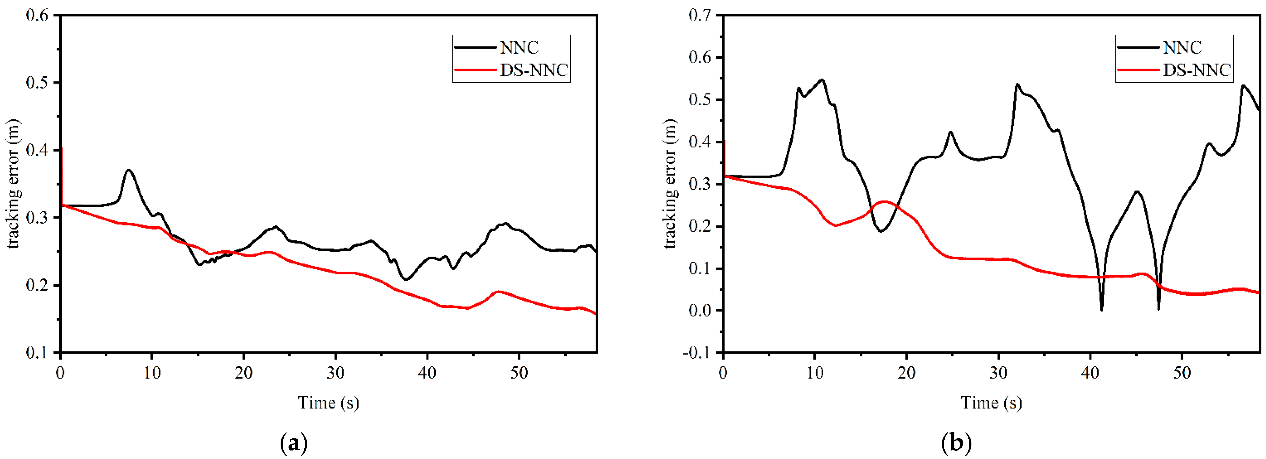
Figure 14.
Comparison of tracking performance. Here the NNC is trained by using a general structure, as shown in Equation (1). (a) Vehicle dynamic model in Case1; (b) vehicle dynamic model in case 3.
Figure 14.
Comparison of tracking performance. Here the NNC is trained by using a general structure, as shown in Equation (1). (a) Vehicle dynamic model in Case1; (b) vehicle dynamic model in case 3.


Table 1.
Vehicle parameters.
| Parameter | Symbol | Value |
|---|---|---|
| Mass | m | 1830 kg |
| Yaw inertia moment | Iz | 3234 kg·m2 |
| Front wheel base | a | 1400 mm |
| Rear wheel base | b | 1650 mm |
| Front axle cornering stiffness | Cf | −125,374 N/rad |
| Rear axle cornering stiffness | Cr | −125,374 N/rad |
Table 2.
Comparison of computation time between MPC and NN controller.
| Controller | Module | Computation Time (s) |
|---|---|---|
| MPC | Longitudinal controller | 11.990 |
| Vehicle dynamic model | 5.740 | |
| Predictive state calculate | 0.988 | |
| QP solver | 9.502 | |
| NNC | Longitudinal controller | 12.735 |
| Vehicle dynamic model | 5.548 | |
| Predictive state calculate | 0.754 | |
| Network | 0.333 |
Table 3.
Path tracking error of MPC and NN controller.
| Deviation | Module | Mean Tracking Error |
|---|---|---|
| Position | MPC | 0.2236 m |
| NN | 0.2234 m | |
| NNFH | 0.2052 m | |
| NNSH | 0.1912 m | |
| Yaw angle | MPC | 0.0299 rad |
| NN | 0.0299 rad | |
| NNFH | 0.0300 rad | |
| NNSH | 0.0299 rad |
Table 4.
Vehicle parameters.
| Parameter | Symbol | Value |
|---|---|---|
| Mass | m | 1140 kg |
| Yaw inertia moment | Iz | 1020 kg·m2 |
| Front wheel base | a | 1165 mm |
| Rear wheel base | b | 1165 mm |
| Front axle cornering stiffness | Cf | −29,517 N/rad |
| Rear axle cornering stiffness | Cr | −29,517 N/rad |
Disclaimer/Publisher’s Note: The statements, opinions and data contained in all publications are solely those of the individual author(s) and contributor(s) and not of MDPI and/or the editor(s). MDPI and/or the editor(s) disclaim responsibility for any injury to people or property resulting from any ideas, methods, instructions or products referred to in the content. |
© 2024 by the authors. Licensee MDPI, Basel, Switzerland. This article is an open access article distributed under the terms and conditions of the Creative Commons Attribution (CC BY) license (https://creativecommons.org/licenses/by/4.0/).
Share and Cite
MDPI and ACS Style
Su, L.; Mao, Y.; Zhang, F.; Lin, B.; Zhang, Y. Deviation Sequence Neural Network Control for Path Tracking of Autonomous Vehicles. Actuators 2024, 13, 101. https://0-doi-org.brum.beds.ac.uk/10.3390/act13030101
AMA Style
Su L, Mao Y, Zhang F, Lin B, Zhang Y. Deviation Sequence Neural Network Control for Path Tracking of Autonomous Vehicles. Actuators. 2024; 13(3):101. https://0-doi-org.brum.beds.ac.uk/10.3390/act13030101
Chicago/Turabian StyleSu, Liang, Yiyuan Mao, Feng Zhang, Baoxing Lin, and Yong Zhang. 2024. "Deviation Sequence Neural Network Control for Path Tracking of Autonomous Vehicles" Actuators 13, no. 3: 101. https://0-doi-org.brum.beds.ac.uk/10.3390/act13030101
Note that from the first issue of 2016, this journal uses article numbers instead of page numbers. See further details here.